Article

Sandwiched Magnetic Coupler for Adjustable Gear Ratio

Department of Mechanical Engineering, National Cheng Kung University, No. 1, University Road, Tainan City 70101, Taiwan
*
Author to whom correspondence should be addressed.
Inventions 2016, 1(3), 18; https://doi.org/10.3390/inventions1030018
Submission received: 28 July 2016 / Revised: 22 August 2016 / Accepted: 24 August 2016 / Published: 1 September 2016

Abstract

:
An innovative design of a magnetic coupler for shaft speed amplification is proposed and verified by experiments. The structure of the proposed magnetic coupler is similar to an infinite-stage gearbox. In addition, the mathematical model of flux density is derived to look into the equation of adjustable gear ratio and effect of speed amplification. Moreover, two sets of experiments, namely verification of gear ratio and observation of stall phenomenon, are built up to examine the capabilities and drawbacks of the proposed variable-gear-ratio magnetic coupler. Three types of gear ratios are presented by theoretical analysis at first and then examined by experiments. The gear ratios for these three specific types between the input and output rotors are 4.75, 5.75 and 10.5, respectively. That is, the rotational speed of the output rotor can be precisely and realistically amplified. Besides, in order to reduce the torque inertia of the outer rotor, a ferrite bush is inserted to the inner side of the core rotor to decrease the flux density in the air gap. On the other hand, the overlapped depth of permanent magnets, which are attached onto the inner rotor and outer rotor, has to be appropriately chosen. The smaller the overlapped depth, the weaker is the magnetic attractive force in the air gap. As long as these two modifications (an inserted ferrite bush and the aforesaid overlapped depth) are validated, the torque inertia of the outer rotor can be significantly reduced. Accordingly, the required power to rotate the outer rotor can be greatly reduced if the overlapped depth is shortened. However, insufficient overlapped depth between the high-speed rotor and low-speed rotor will bring about a stall phenomenon caused by the magnetic attractive force between the high-speed rotor and the low-speed rotor being weaker than the start-up torque inertia. In other words, the reduced overlapped depth can also reduce the start-up torque inertia but stall phenomenon may easily occur.

Graphical Abstract

1. Introduction

Existing variable speed magnetic couplings are available in two or three-tiered versions. Muruganandam et al. changed the operation mode of an existing bevel gear coupling using a two-tiered magnetic coupling to convert contact-based torque transmission to non-contact operation [1], while Andersen used a contact-based cycloidal gear in lieu of non-contact transmission [2]. The three-tiered magnetic coupling was pioneered by Atallah in 2001 [3]. Some of the new designs had drawbacks, while they had a very good magnetic circuit system. This was achieved at the expense of lower torque transmission efficiency and power [4] while some others suffered the opposite effect [5,6]. Another investigation of three-tiered magnetic couplings by Atallah (2004) included a simulation of three different RPM ratios [7]. In the same paper, he suggested ways to get a paired RPM ratio to mitigate the impact of cogging torque. Andersen et al. then switched to the study of power loss by magnetic couplings [8] when Brönn et al. focused on magnetic loss [9]. Cruden et al. explored relationships between the speeds of different rotors [10]. Atallah et al. also reviewed power I/O of their own magnetic coupling designs as well their application in fans and vehicles as an m-CVT (magnetic and continuously variable transmission) [11]. As far as applications are concerned, most authors are interested in fields of greater input power, for example, in the transmission systems of fans and cars. See papers on fans by Frank et al. [12], Abdel-Khalik [13], Chau et al. [14,15] and Fan et al. [16] on automobiles.
In areas other than the search for greater power, Jian et al. [17] improved on the work of Atallah [3] by simplifying the three-tier structure design into a two-tier one while retaining the variable speed feature. This was aimed at ultra-high torque output at low speed. While a lot of attention has been given to greater power or magnetic coupling based reducers, applications involving low power or acceleration have been neglected. This paper presents and tests a design for magnetic couplings useful for acceleration at low power. There are many occasions for the proposed magnetic coupling module to be applied. For example, the proposed three-layer coupling can be applied to drive two mechanisms simultaneously with solely a single power source. More generally, it can be applied to a CVT (Continuously Variable Transmission) system to replace the traditional fixed gear-ratio gearboxes. Especially, for the stage of run-up or run-down period for a rotor/shaft to accelerate or decelerate, the corresponding rotational speed of rotor needs to be continuously variable. The most popularly employed pumps in clean rooms are TMPs (Turbo Molecular Pumps) which do not allow noise, clutch shift, friction or serious vibration. By applying the proposed magnetic coupling to TMPs, the merits, such as electrical energy reduction and the significant downsizing of the overall system, are obvious because a course pump is not necessary any more for the low-speed zone (below 30,000 RPM).

2. Materials and Methods

The variable speed magnetic coupling used in this study has a cross-sectional structure as shown in Figure 1. There are three tiers of rotors: outer, core, and inner. The frame structure of the core rotor is made of aluminum while the ferrite sticks are embedded in the slots of the frame along the circular direction. Also, the inner and outer tiers have radially magnetized permanent magnets.
To get the greatest magnetic coupling force, speed relationships between rotors must meet the requirements of Formula (1) according to a spectrum analysis of the magnetic flux density in the gaps between the inner and core rotors [3]:
Ω h = p l p l n s Ω l n s p l n s Ω c
where Ω c , Ω l , and Ω h , are speed of core, outer (low speed) and inner (high speed) rotors, respectively, p l is the magnet pole pair of the outer rotor magnet and n s is the number of bars in the core rotor. In a case like this, the number of virtual magnet pole pairs in the main magnetic field must be equal to those in the secondary magnetic field:
p l = | p h n s |
where p h the count of magnet pole pairs of the inner rotor. At the same speed, Formula (1) suggests the maximum I/O speed ratio G ^ r can be reached when Ω l = Ω c .
G ^ r = | p l + n s p l n s |
The count of magnetic pole pairs and iron rods in the rotor is determined by the cogging torque factor [18] to mitigate cogging torque at a low rotation speed:
C T = 2 p h n s N c
where N c the least common multiple of magnet count ( 2 p ) and the rotor iron rod count ( n s ) with C T   =   1 the optimum value. Setting the inner rotor magnet pole pair count p h = 4 we can obtain Table 1 based on Formulas (2)–(4).
In this study, the target speed ratio was set to 1:10. Option B of Table 1 was chosen to pair with the count of outer magnets and iron rods. To reach the target ratio of 1:10, input torque must outrun the maximum coupling magnetic moment of inertia between the outer and core rotors before getting the two rotating in the opposite direction during gradual acceleration of the inner rotor. Jang et al. [19] suggest that the maximum magnetic moment of inertia between outer and core rotors can be reduced effectively by inserting a thin ring between the outer and core rotors. The impact of ring thickness on the maximum magnetic moment of inertia is shown in Figure 2. The finite element analysis program Ansoft Maxwell (Ansoft Corporation, Pittsburgh, PA, USA) was used with the parameter settings in Table 2. A 1 mm thick ring was used to ensure machining precision.

3. Results

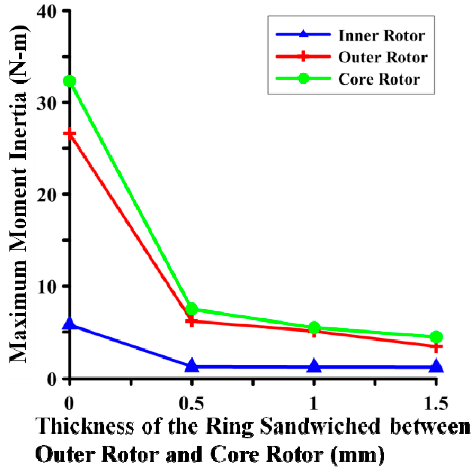
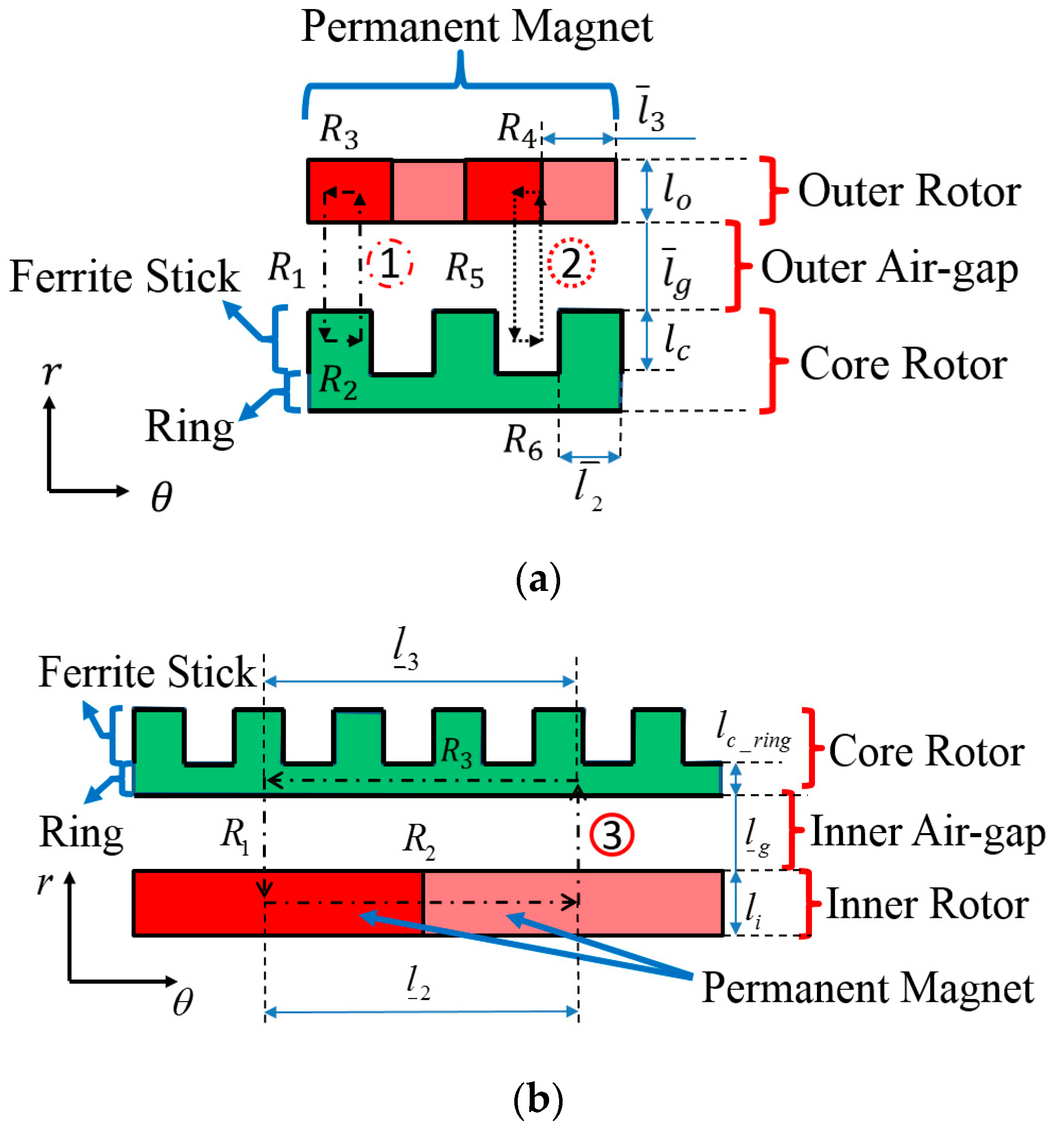
3.1. Magnetic Moment of Inertia Derivation

The magnetic circuit in the outer and inner air gaps is shown in Figure 3. The magnetic line of the magnetomotive force (MMF) path ① ( Λ ¯ max ) passes through magnet, air gap, and iron bar while path ② ( Λ ¯ min ) through magnet and air gap only. As path ① and ② is a periodic distribution function of the outer air gap magnetic conductivity must be a sinusoidal wave with bias. The magnetic lines of force of path ③ ( Λ _ ) go through the magnet, air gap, and iron ring with a constant magnetic conductivity coefficient, so they follow a consistent path.
The magnetic flux density distribution in the inner and outer air gaps is derived with the following two assumptions:
(1)
The magnetic conductivity coefficient of iron rods and the ring is considered infinite ( μ r ).
(2)
here is no flux leakage and fringing effect between iron rods, magnet and iron ring.
Magnetic flux density in the air gap is given by Formula (5) according to MMF conservation:
B g ( θ ) = F m μ 0 g = F m Λ
where B g is the magnetic flux density in the air gap, Λ is the sum of the magnetic conductivity coefficient in paths passed by the MMF, and g is the length of the air gap. Formula (5) can be revised as in Formula (6) and Formula (7) due to the different number of permanent magnets in the inner and outer rotors:
B ¯ g ( θ ) = F ¯ m ( θ ) Λ ¯ ( θ )
B _ g ( θ ) = F _ m ( θ ) Λ _ ( θ )
where B ¯ g ( θ ) and B _ g ( θ ) represent the magnetic flux density function of the outer and inner air gaps, respectively, F ¯ m ( θ ) and F _ m ( θ ) the MMF function of outer and inner air gap, Λ ¯ ( θ ) and Λ _ ( θ ) the magnetic conductivity function of outer and inner air gap as shown in Formula (8) and Formula (9):
Λ _ ( θ ) = 1 2 R _ 1 + R _ 2 + R _ 3 = 1 2 ( l c _ r i n g μ r i μ 0 + l _ g μ 0 + l i μ r m μ 0 ) + l _ 2 μ r m μ 0 + l _ 3 μ r i μ 0
Λ ¯ max = Λ ¯ max + Λ ¯ min 2 + Λ ¯ max Λ ¯ min 2 sin ( n s θ )
where in
Λ ¯ max = 1 2 R ¯ 1 + R ¯ 2 + R ¯ 3 = 1 2 ( l c μ r i μ 0 + l ¯ g μ 0 + l o μ r m μ 0 ) + l ¯ 2 μ r i μ 0 + l ¯ 3 μ r m μ 0
Λ ¯ min = 1 2 R ¯ 5 + R ¯ 4 + R ¯ 6 = 1 2 ( l c μ 0 + l ¯ g μ 0 + l o μ r m μ 0 ) + l ¯ 3 μ r m μ 0 + l ¯ 2 μ 0
where μ 0 , μ r i , and μ r m are the magnetic conductivity of air, iron bar, and magnet, respectively; R is the reluctance at individual points, l c the radial length of iron bar, l ¯ g the radial length of outer air gap, l o the radial length of outer rotor permanent magnet, l ¯ 2 the root arc of iron bar, l ¯ 3 the outer arc length of outer rotor permanent magnet, l c _ r i n g the radial length of iron ring, l _ g the radial length of inner air gap, l i the radial length of inner rotor permanent magnet, l _ 2 the arc length of inner rotor permanent magnet, l _ 3 the arc length of iron ring in the same arc length angle as inner rotor permanent magnet. Due to the weakened magnetic field strength at the permanent magnet border area by the opposing magnetic field, the MMF at this area looks like a trapezoidal, rather than a square wave, as shown in Figure 4.
The trapezoid wave MMF function in the inner and outer air gap is
f ¯ ( θ ) = { F ¯ m θ p l r ¯ π ,   0 θ π p l r ¯ F ¯ m ,   π p l r ¯ θ ( r ¯ 1 ) π p l r ¯ F ¯ m p l r ¯ π [ θ ( r ¯ 1 ) π p l r ¯ ] + F ¯ m   ,   ( r ¯ 1 ) π p l r ¯ θ ( r ¯ + 1 ) π p l r ¯ F ¯ m ,   ( r ¯ + 1 ) π p l r ¯ θ ( 2 r ¯ 1 ) π p l r ¯ F ¯ m p l r ¯ π [ θ ( 2 r ¯ 1 ) π p l r ¯ ] F ¯ m ,   ( 2 r ¯ 1 ) π p l r ¯ θ 2 π p l
f _ ( θ ) = { F _ m θ p h r _ π ,   0 θ π p h r _ F _ m ,   π p h r _ θ ( r _ 1 ) π p h r _ F _ m p h r _ π [ θ ( r _ 1 ) π p h r _ ] + F _ m   ,   ( r _ 1 ) π p h r ¯ θ ( r _ + 1 ) π p h r _ F _ m ,   ( r _ + 1 ) π p h r _ θ ( 2 r _ 1 ) π p h r _ F _ m p h r _ π [ θ ( 2 r _ 1 ) π p h r _ ] F _ m ,   ( 2 r _ 1 ) π p h r _ θ 2 π p h
where f ¯ ( θ ) and f _ ( θ ) is the MMF function of the outer and inner air gap respectively; r ¯ and r _ the normalized design parameters determining the gradient of the trapezoid wave. The Fourier series expansion of the trapezoid wave can be derived with these two functions [20] with the MMF function of the outer and inner air gaps as shown below:
F ¯ ( θ ) = m = 1 , 2 , 3 , f ¯ m sin ( p l m θ )
F _ ( θ ) = m = 1 , 2 , 3 , f _ m sin ( p h m θ )
where f ¯ m and f _ m are expressed as shown below:
f ¯ m = r ¯ ( π m ) 2 F ¯ m ( sin π r ¯ m + sin ( r ¯ 1 ) π r ¯ m sin ( r ¯ + 1 ) π r ¯ m sin ( 2 r ¯ 1 ) π r ¯ m )
f _ m = r _ ( π m ) 2 F _ m ( sin π r _ m + sin ( r _ 1 ) π r _ m sin ( r _ + 1 ) π r _ m sin ( 2 r _ 1 ) π r _ m )
where F ¯ m and F _ m are the MMF of outer and inner rotor magnet respectively, r ¯ is set to 6 and r _ to 15. The MMF need to be doubled as each magnetic circuit will pass through two permanent magnets:
F ¯ m = 2 H c l o
F _ m = 2 H c l i
where H c is the coercive force K A m of magnet (N35). Plug the inner and outer air gap MMFs into Formulas (6) and (7) to get the magnetic flux density function of the inner and outer air gaps as shown below:
B ¯ g ( θ ) = m = 1 , 2 , 3 , f ¯ m sin ( p l m θ ) [ Λ ¯ max + Λ ¯ min 2 + Λ ¯ max Λ ¯ min 2 sin ( n s θ ) ]
B _ g ( θ ) = m = 1 , 2 , 3 , f _ m sin ( p h m θ ) Λ _
See Formulas (22) and (23) for the magnetic moment of inertia of the inner and outer air gaps:
T ¯ ( θ ) = θ 0 θ 1 2 μ 0 B ¯ g 2 ( θ ) d V ¯ = h ¯ l ¯ g 2 μ 0 B ¯ g 2 ( θ )
T _ ( θ ) = θ 0 θ 1 2 μ 0 B _ g 2 ( θ ) d V ¯ = h _ l _ g 2 μ 0 B _ g 2 ( θ )
where T ¯ ( θ ) and T _ ( θ ) are the outer and inner magnetic moment of inertia functions, respectively; V ¯ and V _ the volume of outer and inner air gap, respectively. To explore the reliability of the Fourier series in Formula (20), the experimental result was compared to a simulation outcome using the finite element method in Ansoft Maxwell (Ansoft Corporation, Pittsburgh, PA, USA) based on the index of the mean average percentage error (MAPE) [8] with Formula (24)
M = 1 n t = 1 n | A t F t A t | × 100 .
where A t is the magnetic flux density value of the inner and outer air gaps by the finite element method and F t that done by the Fourier Series with square and trapezoid waves MAPE, see Figure 5a,b. The latter suggests that both the outer and inner air gap magnetic flux density distribution of trapezoid wave is more precise than its square counterpart in terms of MAPE values.

3.2. Dynamic Math Model of the Variable Speed Magnetic Coupling

Figure 6 illustrates the magnetic coupling of Figure 1, plane cut with both parts placed side by side and shown in the axial direction.
T o , T c , and T i are input torque of outer, core, and inner rotor, respectively; T ¯ and T _ are magnetic moment of inertia of outer and inner air gap which block the rotation of rotors, and T ¯ and T _ is the reverse magnetic moment of inertia in the outer and inner air gap.
The torque balancing equation of the core, outer, and inner rotors:
T c = T ¯ ( θ ) + T _ ( θ ) + I c α c
T o = T ¯ ( θ ) + I o α o
T i = T _ ( θ ) + I i α i
where I c , I o , and I i are the rotational inertia of core, outer, and inner rotors; α c , α o and α i the angular acceleration of core, outer, and inner rotors. Formulas (25)–(27) can be converted into Formulas (29)–(31) due to T ¯ and T _ being the corresponding transmitted torque with respect to T ¯ and T _ , respectively:
T c = T ¯ ( θ ) T _ ( θ ) + I c α c
Substitute Formula (20) into Formula (25) to get Formulas (29)–(31):
T c + h ¯ l ¯ g 2 μ 0 B ¯ g 2 ( θ ) + h _ l _ g 2 μ 0 B _ g 2 ( θ ) = I c α c
T o h ¯ l ¯ g 2 μ 0 B ¯ g 2 ( θ ) = I o α o
T i h _ l _ g 2 μ 0 B _ g 2 ( θ ) = I i α i
Assume, (1) constant input torque and (2) steady rotor speed.
In a steady state, we can differentiate Equation (29) with respect to time to get jerk from acceleration as shown in Formula (32):
h ¯ l ¯ g 2 μ 0 d d t B ¯ g 2 ( θ ) + h _ l _ g 2 μ 0 d d t B _ g 2 ( θ ) = 0
Substitute Formula (20) and Formula (21) into Formula (32) to get Formula (33) as shown below:
h ¯ l ¯ g 2 μ 0 d d t { m = 1 , 2 , 3 , f ¯ m sin ( p l m θ ) [ Λ ¯ max + Λ ¯ min 2 + Λ ¯ max Λ ¯ min 2 sin ( n s θ ) ] } 2 + h _ l _ g 2 μ 0 d d t { m = 1 , 2 , 3 , f _ m sin ( p h m θ ) Λ _ } 2 = 0
To simplify the calculation, we took the first term of the Fourier series with MAPE of the inner and outer magnetic flux density to be 30% and converted Formula (33) to Formula (34) as shown below:
h ¯ l ¯ g 2 μ 0 d d t { f ¯ 1 sin ( p l θ ) [ Λ ¯ max + Λ ¯ min 2 + Λ ¯ max Λ ¯ min 2 sin ( n s θ ) ] } 2 + h _ l _ g 2 μ 0 d d t [ f _ 1 sin ( p h θ ) Λ _ ] 2 = 0
We can convert Formula (34) into Formula (35) as magnetic flux density contains the MMF generated by permanent magnet and magnetic conductivity of the inner and outer rotors which means both the MMF and magnetic conductivity rotate with the individual rotors:
h ¯ l ¯ g 2 μ 0 d d t { f ¯ 1 sin ( p l θ p l ω l t ) [ Λ ¯ max + Λ ¯ min 2 + Λ ¯ max Λ ¯ min 2 sin ( n s θ n s ω c t ) ] } 2 + h _ l _ g 2 μ 0 d d t [ f _ 1 sin ( p h θ p h ω h t ) Λ _ ] 2 = 0
where ωl is the speed of outer rotor, ωc is the speed of the core rotor, ωh the speed of inner rotor and B _ g ( θ ) can be rearranged as shown in Formula (36):
h ¯ l ¯ g 2 μ 0 d d t { f ¯ 1 Λ ¯ max + Λ ¯ min 2 sin ( p l θ p l ω l t ) + 1 2 f ¯ 1 Λ ¯ max Λ ¯ min 2 cos [ ( p l n s ) ( θ p l ω l n s ω c p l n s t ) ] 1 2 f ¯ 1 Λ ¯ max Λ ¯ min 2 cos [ ( p l + n s ) ( θ p l ω l + n s ω c p l + n s t ) ] } 2 + h _ l _ g 2 μ 0 d d t [ f _ 1 sin ( p h θ p h ω h t ) Λ _ ] 2 = 0
Differentiate Formula (36) with respect to time to get Formula (37):
h ¯ l ¯ g 2 μ 0 2 B ¯ g ( θ ) { f ¯ 1 Λ ¯ max + Λ ¯ min 2 ( p l ω c p l ω l ) cos ( p l θ p l ω l t ) + 1 2 f ¯ 1 Λ ¯ max Λ ¯ min 2 ( p l n s ) ( ω c p l ω l n s ω c p l n s ) sin [ ( p l n s ) ( θ p l ω l n s ω c p l n s t ) ] 1 2 f ¯ 1 Λ ¯ max Λ ¯ min 2 ( p l + n s ) ( ω c p l ω l + n s ω c p l + n s ) sin [ ( p l + n s ) ( θ p l ω l + n s ω c p l + n s t ) ] } + h _ l _ g 2 μ 0 2 B _ g ( θ ) f _ 1 Λ _ ( p h ω c p h ω h ) cos ( p h θ p h ω h t ) = 0
Formula (37) must be equal to zero as jerk in the steady state is zero. This means constant terms in Formula (37) must be zero which leads to the following constraints:
ω c = ω l
ω c = p l ω l n s ω c p l n s
ω c = p l ω l + n s ω c p l + n s
ω c = ω h
Deduct Formula (39) and Formula (41) from Formula (38) and Formula (40) to get Formula (42) and Formula (43) as shown below:
0 = ω l p l ω l n s ω c p l n s
0 = ω h p l ω l + n s ω c p l + n s
Include Formula (42) to Formula (43) to get Formula (44) as shown below:
ω h = ( p l 2 + n s 2 ) ω l 2 n s 2 ω c p l 2 n s 2
Formula (44) indicates the speed ratio of the variable speed magnetic coupling. Results of combining Formula (44) and Formula (1) can be seen in Figure 7 which are close to what Atallah et al. got [3]. With the inner rotor magnet pole pair ( p h = 4), outer rotor magnet pole pair ( p l = 19), and core rotor iron rod count ( n s = 23) set in this study, the maximum speed ratio ( G ^ r ) given shown by Atallah et al. may reach 1: 10.5 while its counterpart ( G ^ r ) found here may hit 1:11.6. The magnetostatic field analysis and magnetic distribution of this magnetic coupling has been undertaken via Ansoft Maxwell (Ansoft Corporation, Pittsburgh, PA, USA). The main result of computer simulation is concluded by the new figure, Figure 8. In fact, the ferrite sticks embedded in the core rotor play the role of the paths of the magnetic flux to go through. The theoretical saturation level of magnetic flux density of the ferrite sticks is about 1.4 T. However, the actual maximum value in the frame structure of the core rotor is only about 0.5 T. That is, no any magnetic saturation at any device can be found in our work.

4. Discussion

Entity and cross section view of a variable speed magnetic coupling is shown in Figure 9 and Figure 10 where Input #2 is a fixed speed input and Input #1 a variable one. The inner rotor is composed of an aluminum shaft, yoke, and sintered NdFeB (N35), the frame structure of core rotor is made of aluminum while the ferrite sticks are embedded in the slots of the frame along the circular direction. The outer rotor employs a timing belt for transmission and is connected to either one of the two input sources. It is noted that the overlapped depth, shown in Figure 10, is referred to the overlapped length between the magnets (pink) at the inner rotor (indio) and the magnets (pink) at outer rotor (Khaki). The overlapped depth is named as OD hereafter in this paper.

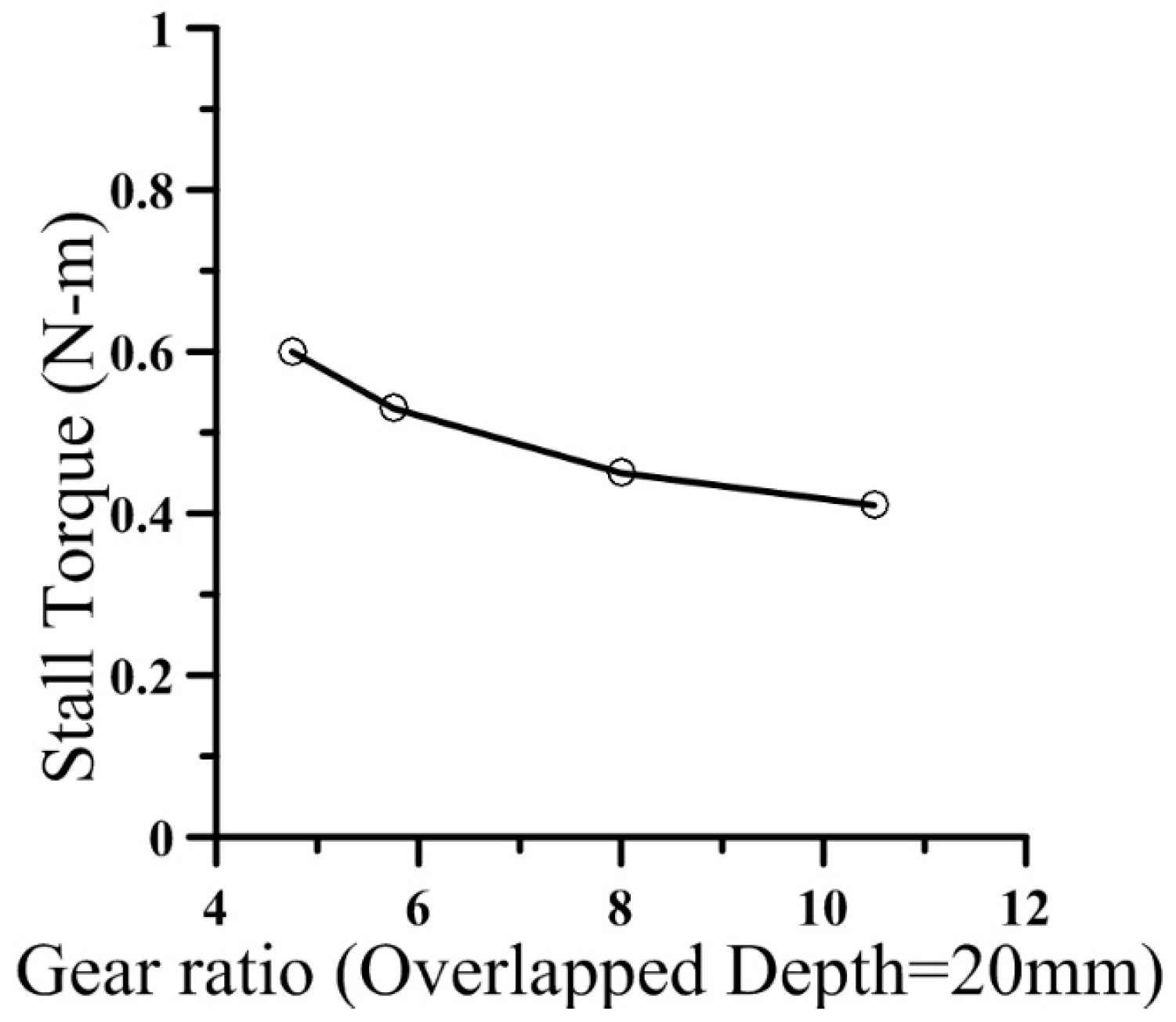
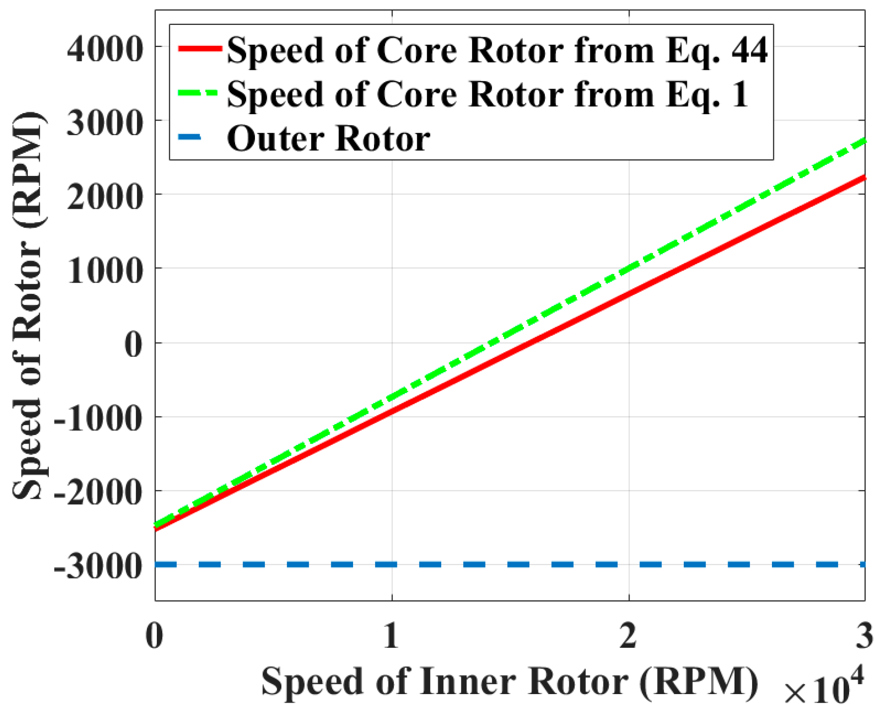
4.1. Verifying the Speed Ratio of the Variable Speed Magnetic Coupling

To verify whether this variable speed magnetic coupling can accomplish the following speed ratio:
(i)
maximum speed ratio ( G ^ r ) at 10.5;
(ii)
speed of inner rotor is 4.75 times that of the outer one when the outer one serves as power input and the inner one as the output end and the core rotor is fixed;
(iii)
speed of inner rotor is 5.75 times that of the core when the core serves as power input and the inner one is the output end and the outer rotor is fixed.
See Table 3 for the speed of individual rotors with an inner rotor magnet and core iron rotor overlap of 20 mm in the experiment setup shown in Figure 11. Figures in row of Mode 1, 2, and 3 are the results with different core and inner rotor speeds which conform with the values derived from Formula (25).

4.2. Speed Ratio Experiment of Variable Speed Magnetic Coupling

Speed ratio experiment of variable speed magnetic coupling are executed in the following steps:
(1)
Outer rotor set to 300 rpm in counterclockwise direction;
(2)
Core rotor set to speed up slowly from 0 to 360 rpm in clockwise direction;
(3)
Outer rotor set to speed up to 420 rpm when the core reaches 360 rpm.
Relationship between speed and frequency in the steps described above is indicated by the solid line in Figure 12.
Calculate the individual inner rotor theoretical output speed using the Atallah [16] speed ratio equation and the one derived in this study based on the actual outer and core rotor speeds obtained by experiment. Figure 12 suggests our experimental figures agree quite closely with those obtained by Atallah. However, some errors exist because we derived the speed ratio formula using only the first term of the Fourier series. The stall condition (dotted line in Figure 12) suggests a coupling effect by the magnetic fields of the permanent magnets in the outer and inner rotors when output torque is weaker than the load.

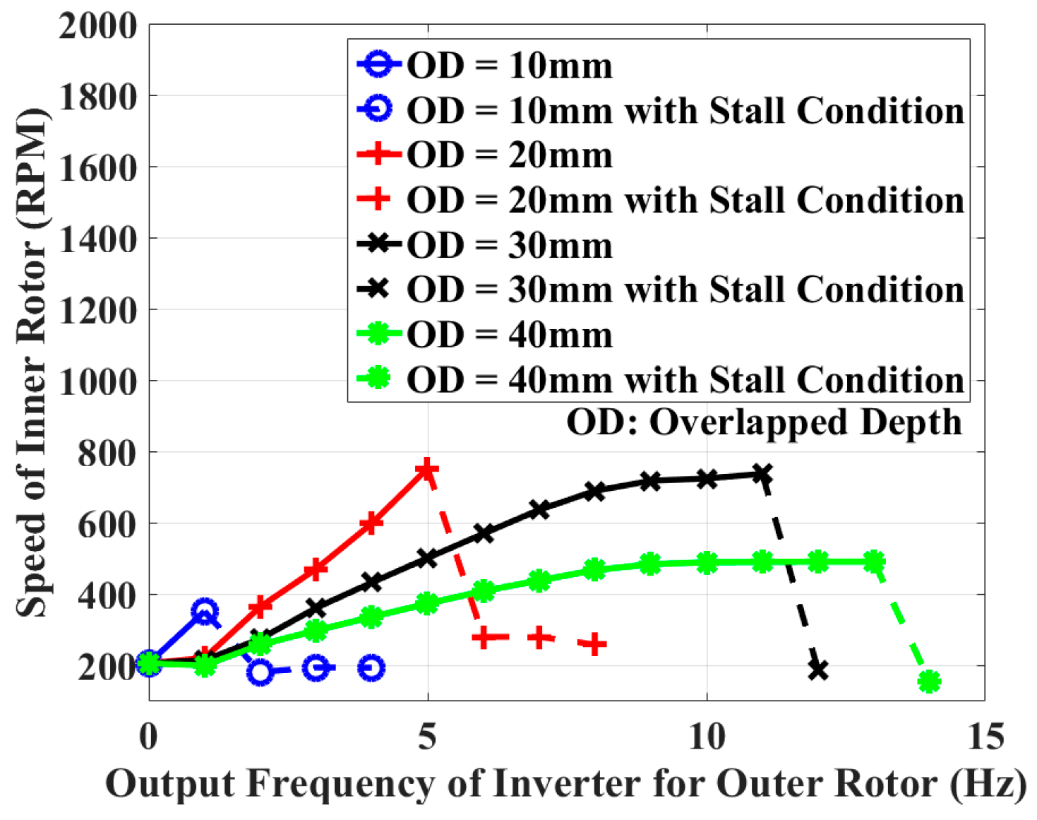
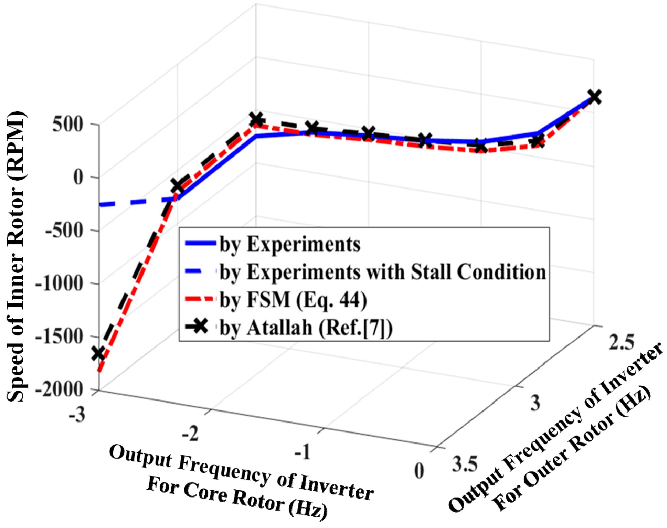
4.3. Stall Condition Experiment of Variable Speed Magnetic Coupling

The greater overlapping area between the permanent magnets of inner and outer rotors makes the coupling effect between rotors as stronger as it can get. The output speed of inner rotor at different overlap depths with fixed core rotor input frequency and increasing outer rotor frequency (by experiment steps) given below are shown in Figure 13:
(1)
Set core rotor speed to 420 rpm.
(2)
Keep core rotor speed constant and increment the outer rotor input frequency until stalling is encountered.
The solid line in Figure 13 shows the normal output speed of inner rotor, while the dotted line indicates a stall. Figure 13 suggests stall occurs only when the coupling area between outer and inner rotor permanent magnet is up and the outer rotor is also spinning fast. On the other hand, the bigger overlap of the inner rotor will lead to lower output speed as the magnetic moment of inertia in the air gap goes up due to greater coupling force between the inner and outer rotor permanent magnets. To be more detailed, the stall torque versus the gear ratio is shown in Figure 14. It can be observed the stall torque is slightly reduced as the gear ratio is increased. That is, the higher the gear ratio, the less torque can be transmitted at the high speed rotor, i.e., inner rotor. There are two conclusions from this experiment:
(1)
The variable speed magnetic coupling presented here conforms with the initial target of maximum speed ratio ( G ^ r ) at 10.5 and its speed modulating function has been proved correct.
(2)
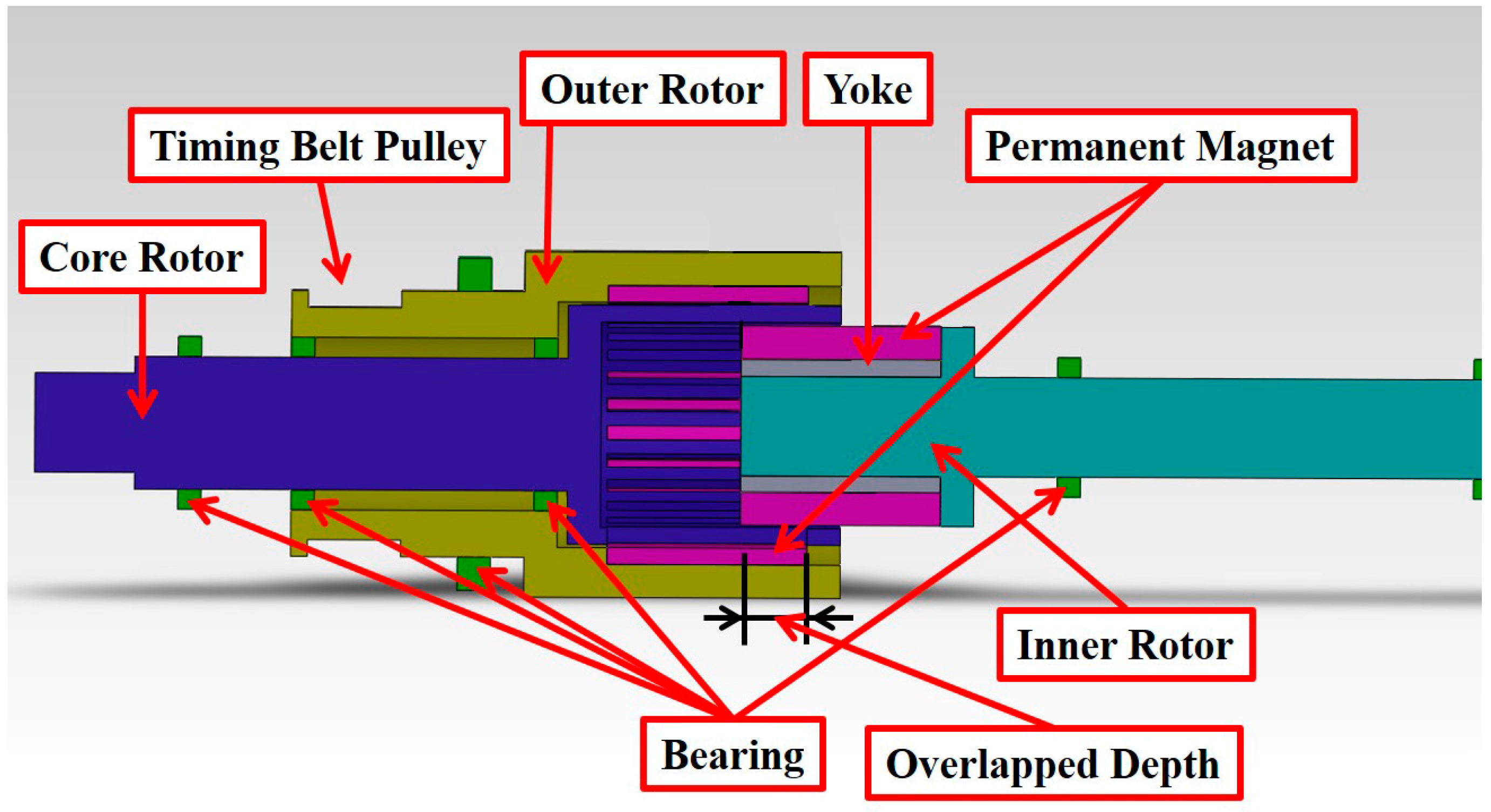
A smaller overlap of the inner rotor reduces the magnetic moment of inertia in the air gap but increases the likelihood of stalling.

5. Conclusions

The variable speed magnetic coupling described in this study was designed after careful calculation of the number of magnet pole pairs needed for the permanent magnets of the inner and outer rotors and iron rods in the core. The result of the design was a variable speed magnetic coupling with a maximum speed ratio of 10.5. Calculation of the magnetic energy in the air gap is based on magnetic flux density derivation of the magnetic moment of the inertia equation which was used to establish a dynamic formula for individual rotors. The results were used to develop the speed ratio equation based on the concept of jerk. The experimental results confirmed the theoretical conclusions and also suggested that a shorter inner rotor overlap may effectively reduce the magnetic moment of inertia in the air gap at the expense of a greater likelihood of stalling.

Acknowledgments

This research was supported in part by the Ministry of Science and Technology (Taiwan) with Grant MOST 103-2221-E-006-046-MY3, for which the authors express their sincere appreciation.

Author Contributions

Foo-Hong Leong undertakes the experiments and analyzes the data; Nan-Chyuan Tsai designs the structure of research, contributes to the discussion, and revises the manuscript; Hsin-Lin Chiu writes the manuscript for the first version.

Conflicts of Interest

The authors declare no conflict of interest.

References

  1. Muruganandam, G.; Padma, S.; Slvakumar, P. Design and Implementation of a Novel Magnetic Bevel Gear. CEAI 2013, 15, 30–37. [Google Scholar]
  2. Rgensen, F.T.J.; Andersen, T.O.; Rasmussen, P.O. The Cycloid Permanent Magnetic Gear. IEEE Trans. Ind. Appl. 2008, 44, 1659–1665. [Google Scholar] [CrossRef]
  3. Atallah, K.; Howe, D. A novel high-performance magnetic gear. IEEE Trans. Magn. 2001, 37, 2844–2846. [Google Scholar] [CrossRef]
  4. Hesmondhalgh, D.E.; Tipping, D. A multi-element magnetic gear. IEEE Proc. B Electr. Power Appl. 1980, 127. [Google Scholar] [CrossRef]
  5. Tsurumoto, K.; Kikuchi, S. A new magnetic gear using permanent magnet. IEEE Trans. Magn. 1987, 23. [Google Scholar] [CrossRef]
  6. Ikuta, K.; Makita, S.; Arimoto, S. Non-contact magnetic gear for micro transmission mechanism. In Proceedings of the IEEE Conference on Micro electro mechanical systems, MEM’91, Nara, Japan, 2 January 1991; pp. 125–130.
  7. Atallah, K.; Calverley, S.D.; Howe, D. Design, Analysis and Realisation of a High-Performance Magnetic Gear. IEE Proc. Electr. Power Appl. 2004, 151, 135–143. [Google Scholar] [CrossRef]
  8. Rasmussen, P.O.; Andersen, T.O.; Rgensen, F.T.J.; Nielsen, O. Development of a High-Performance Magnetic Gear. IEEE Trans. Ind. Appl. 2005, 41, 764–770. [Google Scholar] [CrossRef]
  9. Brönn, L.; Wang, R.-J.; Kamper, M. Development of a Shutter Type Magnetic Gear. In Proceedings of the 19th Southern African Universities Power Engineering Conference SAUPEC 2010, University of the Witwatersrand, Johannesburg, South Africa, 28–29 January 2010.
  10. Shah, L.; Cruden, A.; Williams, B.W. A Variable Speed Magnetic Gear Box Using Contra-Rotating Input Shafts. IEEE Trans. Magn. 2011, 47, 431–438. [Google Scholar] [CrossRef]
  11. Atallah, K.; Wang, J.; Calverley, S.D.; Duggan, S. Design and Operation of a Magnetic Continuously Variable Transmission. IEEE Trans. Ind. Appl. 2012, 48, 1288–1295. [Google Scholar] [CrossRef]
  12. Frank, N.W.; Toliyat, H.A. Gearing Ratios of a Magnetic Gear for Wind Turbines. In Proceedings of the Electric Machines and Drives Conference, Miami, FL, USA, 3–6 May 2009; pp. 1224–1230.
  13. Abdel-Khalik, A.; Ahmed, S.; Massoud, A.; Elserougi, A. Magnetic Gearbox with an Electric Power Output Port and Fixed Speed Ratio for Wind Energy Applications. J. Energy Power Eng. 2013, 7, 1141–1149. [Google Scholar]
  14. Chau, K.; Zhang, D.; Jiang, J.; Liu, C.; Zhang, Y. Design of a Magnetic-Geared Outer-Rotor Permanent-Magnet Brushless Motor for Electric Vehicles. IEEE Trans. Magn. 2007, 43, 2504–2506. [Google Scholar] [CrossRef] [Green Version]
  15. Chau, K.-T.; Liu, C.-H. Electromagnetic Design of a New Electrically Controlled Magnetic Variable-Speed Gearing Machine. Energies 2014, 7, 1539–1554. [Google Scholar] [Green Version]
  16. Fan, Y.; Jiang, H.; Cheng, M.; Wang, Y. An Improved Magnetic-Geared Permanent Magnet in-Wheel Motor for Electric Vehicles. In Proceedings of the Vehicle Power and Propulsion Conference (VPPC), Lille, France, 1–3 September 2010.
  17. Jian, L.-N.; Shi, Y.-J.; Liu, C.; Xu, G.-Q.; Gong, Y.; Chan, C.-C. A Novel Dual-Permanent-Magnet-Excited Machine for Low-Speed Large-Torque Applications. IEEE Trans. Magn. 2013, 49, 2381–2384. [Google Scholar] [CrossRef]
  18. Zhu, Z.-Q.; Howe, D. Influence of Design Parameters on Cogging Torque in Permanent Magnet Machines. IEEE Trans. Energy Convers. 2000, 15, 407–412. [Google Scholar] [CrossRef]
  19. Jang, D.-K.; Chang, J.-H. Effect of Stationary Pole Pieces with Bridge on Electromagnetic and Mechanical Performance of a Coaxial Magnetic Gear. J. Magn. 2013, 18, 207–211. [Google Scholar] [CrossRef]
  20. Dajaku, G.; Gerling, D. Stator Slotting Effect on the Magnetic Field Distribution of Salient Pole Synchronous Permanent-Magnet Machines. IEEE Trans. Magn. 2010, 46, 3676–3683. [Google Scholar] [CrossRef]
Figure 1. Structure of the variable speed of magnetic coupling.
Inventions 01 00018 g001
Figure 2. Impact of ring thickness on the maximum magnetic moment of inertia.
Inventions 01 00018 g002
Figure 3. (a) Outer air gap magnetic circuit and (b) inner air gap magnetic circuit.
Inventions 01 00018 g003
Figure 4. Magnetomotive force distribution of permanent magnet MMF in the air gap.
Inventions 01 00018 g004
Figure 5. MAPE of square and trapezoid waves, numerical and finite element methods. (a) At the outer air gap; (b) At the inner air gap.
Inventions 01 00018 g005
Figure 6. Free body diagram between rotors of variable speed magnetic coupling.
Inventions 01 00018 g006
Figure 7. Speed of individual rotors of a variable speed magnetic coupling.
Inventions 01 00018 g007
Figure 8. Magnetostatic field analysis (Ansoft Maxwell).
Inventions 01 00018 g008
Figure 9. Laboratory setup of the variable speed magnetic coupling.
Inventions 01 00018 g009
Figure 10. Cross section of the variable speed magnetic coupling.
Inventions 01 00018 g010
Figure 11. Experimental setup.
Inventions 01 00018 g011
Figure 12. Inner rotor speed at different input speeds (with 20 mm overlap depth).
Inventions 01 00018 g012
Figure 13. Changes of output speed of the inner rotor at different overlap depths.
Inventions 01 00018 g013
Figure 14. Stall torque versus gear ratio.
Inventions 01 00018 g014
Table 1. Maximum speed with p h = 4 .
Options p h n s p l 2 × p h N c C T G ^ r
A42218888210
B423198184110.5
C42420824811
D425218200111.5
Table 2. Parameters of variable speed magnetic coupling.
ParameterSymbolValue
Radial Length of Ferrite Rods l c 4 mm
Radial Length of Air Gap l ¯ g , l _ g 1 mm
Radial Length of Outer-rotor Magnets l o 5 mm
Arc Width of Ferrite Rods on the Inner Side l ¯ 2 4.23 mm
Arc Width of Outer-rotor Magnets on the Outer Side l ¯ 3 6.95 mm
Thickness of Ring l c _ r i n g 1 mm
Radial Length of Inner-rotor Magnets l i 10 mm
Arc Width of Inner-rotor Magnets on the Inside l _ 2 15.7 mm
Arc Width of Ring with the Same Arc Angle with Inner-rotor Magnets l _ 3 25.13 mm
Relative Permeability of Ferrite Rods/Ring μ r i 5000
Relative Permeability of Magnets μ r m 1.05
Permeability of Vacuum μ 0 4 π   ×   10 7 H / m
Coercive Force of N35 H c 955 K A / m
Table 3. Speed of individual rotors in three different operation modes.
Operation Mode ω l ω c ω h Gear Ratio
Rotational SpeedRotational SpeedRotational Speed
148.83 RPM−48.91 RPM−511.32 RPM10.5
285.94 RPM0 RPM−409.15 RPM4.75
30 RPM−109.78 RPM−630.24 RPM5.75

