

Conditional Generative Models for Dynamic Trajectory Generation and Urban Driving


Abstract
1. Introduction
- A formulation for dynamic trajectory generation utilizing nominal global plan representations and local semantic scene models.
- We provide an in-depth analysis on the performance benefits of using graphical methods to represent coarse plans.
- We release two datasets with over 13,000 synchronized global plan and semantic scene representations. In contrast to existing datasets, our data can enable research directions for path planning with fewer priors.
- The code repositories for the nominal planner and dynamic trajectory generation are made open source and publicly available (https://github.com/AutonomousVehicleLaboratory/gps_navigation, accessed on 26 July 2023,https://github.com/AutonomousVehicleLaboratory/coarse_av_cgm.git, accessed on 26 July 2023).
2. Related Work
2.1. HD/Vector Maps
2.2. Lightweight Maps
2.3. Scene Representations
3. Methods
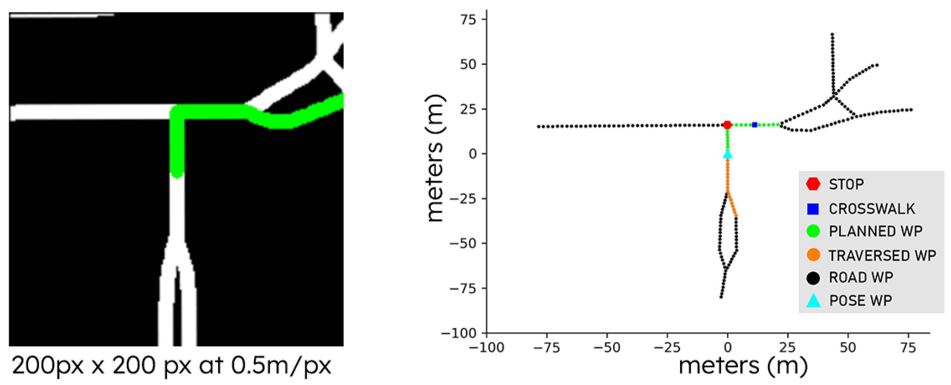
3.1. Global Planning
3.2. Semantic Scene Representation
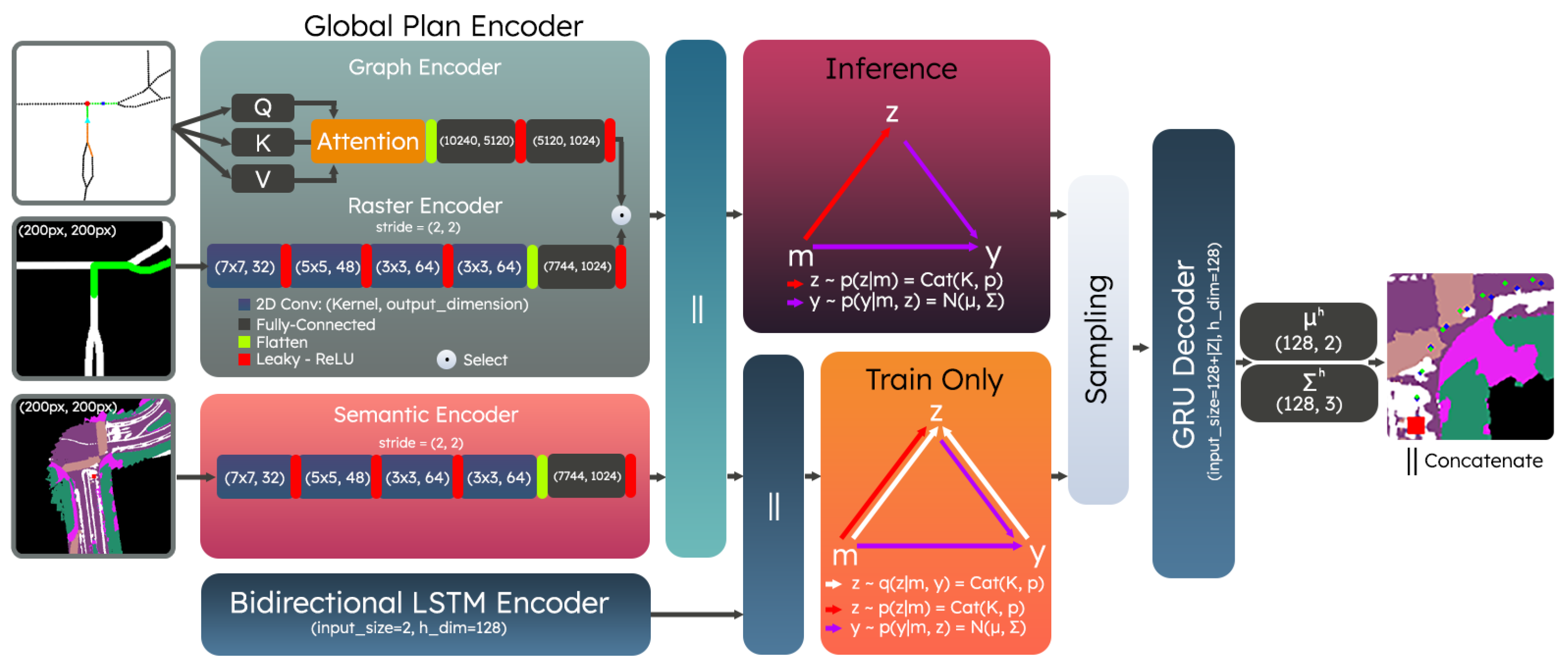
3.3. Conditional Generative Models
4. Experiments and Data
4.1. Datasets
4.2. Platform and Hardware Requirements
4.3. Metrics
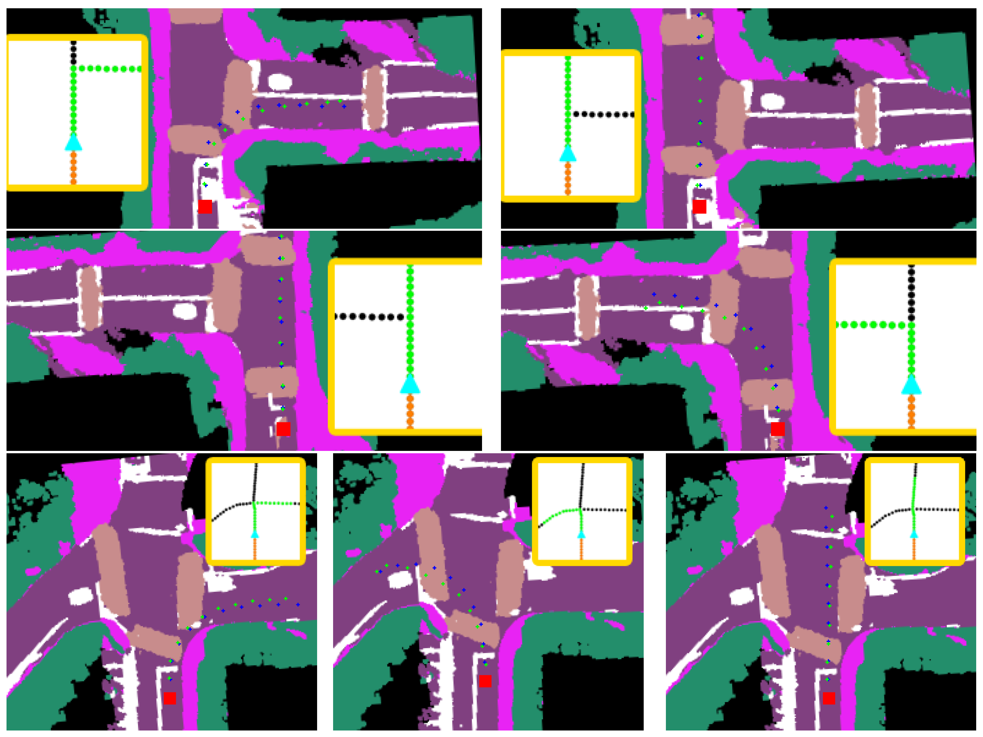
4.4. Results
4.4.1. Ablation Study: Waypoint Density
4.4.2. Ablation Study: Rasterized and Graph Representations
4.5. Discussion
5. Conclusions
Author Contributions
Funding
Institutional Review Board Statement
Informed Consent Statement
Data Availability Statement
Conflicts of Interest
Abbreviations
| HD | High Definition |
| OSM | OpenStreetMaps |
| ROS | Robot Operating System |
| LiDAR | Light Detection and Ranging |
| GNSS | Global Navigation Satellite System |
| XML | Extensible Markup Language |
| CNN | Convolutional neural network |
| CVAE | Conditional Variational Autoencoder |
| KL | Kullback–Leibler |
| DAC | Driveable Area Compliance |
| ADE | Average Displacement Error |
| FDE | Final Displacement Error |
| MDE | Maximum Displacement Error |
| IMU | Inertial Measurement Unit |
Appendix A. Data
Data Collection Process

Appendix B. Experiments
Metrics
References
- Hart, P.E.; Nilsson, N.J.; Raphael, B. A Formal Basis for the Heuristic Determination of Minimum Cost Paths. IEEE Trans. Syst. Sci. Cybern. 1968, 4, 100–107. [Google Scholar] [CrossRef]
- Máttyus, G.; Luo, W.; Urtasun, R. Deeproadmapper: Extracting road topology from aerial images. In Proceedings of the 2017 IEEE International Conference on Computer Vision (ICCV), Venice, Italy, 22–29 October 2017; pp. 3458–3466. [Google Scholar] [CrossRef]
- Büchner, M.; Zürn, J.; Todoran, I.G.; Valada, A.; Burgard, W. Learning and Aggregating Lane Graphs for Urban Automated Driving. arXiv 2023, arXiv:2302.06175. [Google Scholar]
- Zhou, Y.; Takeda, Y.; Tomizuka, M.; Zhan, W. Automatic Construction of Lane-level HD Maps for Urban Scenes. In Proceedings of the 2021 IEEE/RSJ International Conference on Intelligent Robots and Systems (IROS), Prague, Czech Republic, 27 September–1 October 2021; pp. 6649–6656. [Google Scholar] [CrossRef]
- Homayounfar, N.; Ma, W.C.; Lakshmikanth, S.K.; Urtasun, R. Hierarchical Recurrent Attention Networks for Structured Online Maps. In Proceedings of the 2018 IEEE/CVF Conference on Computer Vision and Pattern Recognition, Salt Lake City, UT, USA, 18–23 June 2018; pp. 3417–3426. [Google Scholar] [CrossRef]
- Liu, Y.; Yuan, T.; Wang, Y.; Wang, Y.; Zhao, H. VectorMapNet: End-to-end Vectorized HD Map Learning. In Proceedings of the International Conference on Machine Learning, PMLR, Honolulu, HI, USA, 23–29 July 2023. [Google Scholar]
- Liao, B.; Chen, S.; Wang, X.; Cheng, T.; Zhang, Q.; Liu, W.; Huang, C. MapTR: Structured Modeling and Learning for Online Vectorized HD Map Construction. In Proceedings of the International Conference on Learning Representations, Kigali, Rwanda, 1–5 May 2023. [Google Scholar]
- Li, T.; Chen, L.; Geng, X.; Wang, H.; Li, Y.; Liu, Z.; Jiang, S.; Wang, Y.; Xu, H.; Xu, C.; et al. Topology Reasoning for Driving Scenes. arXiv 2023, arXiv:2304.05277. [Google Scholar]
- Paz, D.; Zhang, H.; Christensen, H.I. TridentNet: A Conditional Generative Model for Dynamic Trajectory Generation. In Intelligent Autonomous Systems 16; Ang, M.H., Jr., Asama, H., Lin, W., Foong, S., Eds.; Springer: Cham, Switzerland, 2022; pp. 403–416. [Google Scholar] [CrossRef]
- Paz, D.; Xiang, H.; Liang, A.; Christensen, H.I. TridentNetV2: Lightweight Graphical Global Plan Representations for Dynamic Trajectory Generation. In Proceedings of the 2022 International Conference on Robotics and Automation (ICRA), Philadelphia, PA, USA, 23–27 May 2022; pp. 9265–9271. [Google Scholar] [CrossRef]
- Kato, S.; Takeuchi, E.; Ishiguro, Y.; Ninomiya, Y.; Takeda, K.; Hamada, T. An Open Approach to Autonomous Vehicles. IEEE Micro 2015, 35, 60–68. [Google Scholar] [CrossRef]
- Apollo: An Open Autonomous Driving Platform. 2017. Available online: https://github.com/ApolloAuto/apollo (accessed on 29 June 2023).
- Christensen, H.; Paz, D.; Zhang, H.; Meyer, D.; Xiang, H.; Han, Y.; Liu, Y.; Liang, A.; Zhong, Z.; Tang, S. Autonomous Vehicles for Micro-Mobility. Auton. Intell. Syst. 2021, 1, 1–35. [Google Scholar] [CrossRef]
- Bansal, M.; Krizhevsky, A.; Ogale, A. ChauffeurNet: Learning to Drive by Imitating the Best and Synthesizing the Worst. arXiv 2018, arXiv:1812.03079. [Google Scholar]
- Zeng, W.; Luo, W.; Suo, S.; Sadat, A.; Yang, B.; Casas, S.; Urtasun, R. End-to-end interpretable neural motion planner. In Proceedings of the IEEE/CVF Conference on Computer Vision and Pattern Recognition (CVPR), Long Beach, CA, USA, 15–20 June 2019; pp. 8660–8669. [Google Scholar] [CrossRef]
- Ivanovic, B.; Elhafsi, A.; Rosman, G.; Gaidon, A.; Pavone, M. Mats: An interpretable trajectory forecasting representation for planning and control. arXiv 2020, arXiv:2009.07517. [Google Scholar]
- Jiang, B.; Chen, S.; Xu, Q.; Liao, B.; Chen, J.; Zhou, H.; Zhang, Q.; Liu, W.; Huang, C.; Wang, X. VAD: Vectorized Scene Representation for Efficient Autonomous Driving. arXiv 2023, arXiv:2303.12077. [Google Scholar]
- Hu, Y.; Yang, J.; Chen, L.; Li, K.; Sima, C.; Zhu, X.; Chai, S.; Du, S.; Lin, T.; Wang, W.; et al. Planning-oriented Autonomous Driving. In Proceedings of the IEEE/CVF Conference on Computer Vision and Pattern Recognition, Vancouver, BC, Canada, 18–22 June 2023; pp. 17853–17862. [Google Scholar]
- Zhang, Z.; Liniger, A.; Dai, D.; Yu, F.; Van Gool, L. End-to-End Urban Driving by Imitating a Reinforcement Learning Coach. In Proceedings of the IEEE/CVF International Conference on Computer Vision (ICCV), Montreal, QC, Canada, 10–17 October 2021. [Google Scholar] [CrossRef]
- Chen, D.; Krähenbühl, P. Learning from all vehicles. In Proceedings of the IEEE/CVF Conference on Computer Vision and Pattern Recognition CVPR, New Orleans, LA, USA, 19–24 June 2022. [Google Scholar]
- Chitta, K.; Prakash, A.; Geiger, A. NEAT: Neural Attention Fields for End-to-End Autonomous Driving. In Proceedings of the International Conference on Computer Vision (ICCV), Virtual, 11–17 October 2021. [Google Scholar]
- Caesar, H.; Kabzan, J.; Tan, K.S.; Fong, W.K.; Wolff, E.; Lang, A.; Fletcher, L.; Beijbom, O.; Omari, S. nuplan: A closed-loop ml-based planning benchmark for autonomous vehicles. arXiv 2021, arXiv:2106.11810. [Google Scholar]
- Dosovitskiy, A.; Ros, G.; Codevilla, F.; Lopez, A.; Koltun, V. CARLA: An Open Urban Driving Simulator. In Proceedings of the 1st Annual Conference on Robot Learning, Mountain View, CA, USA, 13–15 November 2017; Levine, S., Vanhoucke, V., Goldberg, K., Eds.; PMLR: New York, NY, USA, 2017; Volume 78, pp. 1–16. [Google Scholar]
- Rong, G.; Shin, B.H.; Tabatabaee, H.; Lu, Q.; Lemke, S.; Možeiko, M.; Boise, E.; Uhm, G.; Gerow, M.; Mehta, S.; et al. LGSVL Simulator: A High Fidelity Simulator for Autonomous Driving. In Proceedings of the 2020 IEEE 23rd International conference on intelligent transportation systems (ITSC), Rhodes, Greece, 20–23 September 2020; pp. 1–6. [Google Scholar] [CrossRef]
- Hecker, S.; Dai, D.; Van Gool, L. Learning accurate, comfortable and human-like driving. arXiv 2019, arXiv:1903.10995. [Google Scholar]
- Amini, A.; Rosman, G.; Karaman, S.; Rus, D. Variational End-to-End Navigation and Localization. In Proceedings of the 2019 International Conference on Robotics and Automation (ICRA), Montreal, QC, Canada, 20–24 May 2019; pp. 8958–8964. [Google Scholar] [CrossRef]
- Hecker, S.; Dai, D.; Van Gool, L. End-to-End Learning of Driving Models with Surround-View Cameras and Route Planners. In Proceedings of the Computer Vision—ECCV 2018, Munich, Germany, 8–14 September 2018; Ferrari, V., Hebert, M., Sminchisescu, C., Weiss, Y., Eds.; Springer: Cham, Switzerland, 2018; Volume 11211, pp. 435–453. [Google Scholar] [CrossRef]
- Casas, S.; Sadat, A.; Urtasun, R. MP3: A Unified Model to Map, Perceive, Predict and Plan. In Proceedings of the 2021 IEEE/CVF Conference on Computer Vision and Pattern Recognition (CVPR), Nashville, TN, USA, 20–25 June 2021; pp. 14403–14412. [Google Scholar] [CrossRef]
- Hawke, J.; Shen, R.; Gurau, C.; Sharma, S.; Reda, D.; Nikolov, N.; Mazur, P.; Micklethwaite, S.; Griffiths, N.; Shah, A.; et al. Urban Driving with Conditional Imitation Learning. In Proceedings of the 2020 IEEE International Conference on Robotics and Automation (ICRA), Paris, France, 31 May 2020; pp. 251–257. [Google Scholar] [CrossRef]
- Can, Y.B.; Liniger, A.; Unal, O.; Paudel, D.; Van Gool, L. Understanding Bird’s-Eye View of Road Semantics Using an Onboard Camera. IEEE Robot. Autom. Lett. 2022, 7, 3302–3309. [Google Scholar] [CrossRef]
- Dwivedi, I.; Malla, S.; Chen, Y.T.; Dariush, B. Bird’s eye view segmentation using lifted 2D semantic features. In Proceedings of the British Machine Vision Conference (BMVC), London, UK, 22–25 November 2021; pp. 6985–6994. [Google Scholar]
- Paz, D.; Zhang, H.; Li, Q.; Xiang, H.; Christensen, H.I. Probabilistic semantic mapping for urban autonomous driving applications. In Proceedings of the 2020 IEEE/RSJ International Conference on Intelligent Robots and Systems (IROS), Vegas, NV, USA, 24 October 2020; pp. 2059–2064. [Google Scholar] [CrossRef]
- Vaswani, A.; Shazeer, N.; Parmar, N.; Uszkoreit, J.; Jones, L.; Gomez, A.N.; Kaiser, U.; Polosukhin, I. Attention is All You Need. In Proceedings of the 31st International Conference on Neural Information Processing Systems, Red Hook, NY, USA, 4–9 December 2017; pp. 6000–6010. [Google Scholar]
- Sohn, K.; Lee, H.; Yan, X. Learning Structured Output Representation using Deep Conditional Generative Models. In Proceedings of the 28th International Conference on Neural Information Processing Systems, Montreal, QB, Canada, 7–12 December 2015; Cortes, C., Lawrence, N., Lee, D., Sugiyama, M., Garnett, R., Eds.; MIT Press: Cambridge, MA, USA, 2015; Volume 2, pp. 3483–3491. [Google Scholar]
- Salzmann, T.; Ivanovic, B.; Chakravarty, P.; Pavone, M. Trajectron++: Dynamically-feasible trajectory forecasting with heterogeneous data. In Proceedings of the Computer Vision–ECCV 2020: 16th European Conference, Glasgow, UK, 23–28 August 2020; Vedaldi, A., Bischof, H., Brox, T., Frahm, J.M., Eds.; Springer: Cham, Switzerland, 2020; Volume 12363, pp. 683–700. [Google Scholar] [CrossRef]
- Cho, K.; van Merriënboer, B.; Gulcehre, C.; Bahdanau, D.; Bougares, F.; Schwenk, H.; Bengio, Y. Learning Phrase Representations using RNN Encoder–Decoder for Statistical Machine Translation. In Proceedings of the 2014 Conference on Empirical Methods in Natural Language Processing (EMNLP), Doha, Qatar, 25–29 October 2014; pp. 1724–1734. [Google Scholar] [CrossRef]
- Xia, X.; Meng, Z.; Han, X.; Li, H.; Tsukiji, T.; Xu, R.; Zheng, Z.; Ma, J. An automated driving systems data acquisition and analytics platform. Transp. Res. Part C: Emerg. Technol. 2023, 151, 104120. [Google Scholar] [CrossRef]
- Gupta, A.; Johnson, J.; Fei-Fei, L.; Savarese, S.; Alahi, A. Social GAN: Socially Acceptable Trajectories with Generative Adversarial Networks. In Proceedings of the 2018 IEEE/CVF Conference on Computer Vision and Pattern Recognition, Salt Lake City, UT, USA, 18–23 June 2018; pp. 2255–2264. [Google Scholar] [CrossRef]
- Fernando, T.; Denman, S.; Sridharan, S.; Fookes, C. GD-GAN: Generative Adversarial Networks for Trajectory Prediction and Group Detection in Crowds. In Proceedings of the Computer Vision—ACCV 2018, Perth, Australia, 2–6 December 2018; Jawahar, C.V., Li, H., Mori, G., Schindler, K., Eds.; Springer: Cham, Switzerland, 2019; Volume 11361, pp. 314–330. [Google Scholar] [CrossRef]
- Wilson, B.; Qi, W.; Agarwal, T.; Lambert, J.; Singh, J.; Khandelwal, S.; Pan, B.; Kumar, R.; Hartnett, A.; Pontes, J.K.; et al. Argoverse 2: Next Generation Datasets for Self-driving Perception and Forecasting. In Neural Information Processing Systems Track on Datasets and Benchmarks (NeurIPS Datasets and Benchmarks 2021). arXiv 2021, arXiv:2301.00493. [Google Scholar]
- Delseny, H.; Gabreau, C.; Gauffriau, A.; Beaudouin, B.; Ponsolle, L.; Alecu, L.; Bonnin, H.; Beltran, B.; Duchel, D.; Ginestet, J.B.; et al. White Paper Machine Learning in Certified Systems. arXiv 2021, arXiv:2103.10529. [Google Scholar]


| Method | ADE ↓ | ADE ↓ | FDE ↓ | MDE ↓ |
|---|---|---|---|---|
| OSM-H10 | ||||
| OSM-H15 | 2.341875 | 0.753802 | 6.127183 |
| Method | ADE ↓ | ADE ↓ | FDE ↓ | MDE ↓ | DAC ↑ | DAC ↑ |
|---|---|---|---|---|---|---|
| OSM Raster | 1.056245 | 2.447714 | 2.494614 | 0.849162 | 0.934218 | |
| OSM ATT w/PF | 1.365685 | 0.538815 | 2.852894 | 3.047669 | 0.892321 | 0.933054 |
| OSM ATT w/SPF | 0.353576 | 0.944642 | ||||
| OSM ATT w/SCPF | 1.131581 | 0.388303 | 2.717636 | 2.795832 | 0.905864 | 0.942408 |
| Method | ADE ↓ | ADE ↓ | FDE ↓ | MDE ↓ | DAC ↑ | DAC ↑ |
|---|---|---|---|---|---|---|
| OSM Raster | 1.793062 | 0.673450 | 3.672231 | 3.728120 | 0.858367 | 0.913147 |
| OSM ATT w/SPF |
Disclaimer/Publisher’s Note: The statements, opinions and data contained in all publications are solely those of the individual author(s) and contributor(s) and not of MDPI and/or the editor(s). MDPI and/or the editor(s) disclaim responsibility for any injury to people or property resulting from any ideas, methods, instructions or products referred to in the content. |
© 2023 by the authors. Licensee MDPI, Basel, Switzerland. This article is an open access article distributed under the terms and conditions of the Creative Commons Attribution (CC BY) license (https://creativecommons.org/licenses/by/4.0/).
Share and Cite
Paz, D.; Zhang, H.; Xiang, H.; Liang, A.; Christensen, H.I. Conditional Generative Models for Dynamic Trajectory Generation and Urban Driving. Sensors 2023, 23, 6764. https://doi.org/10.3390/s23156764
Paz D, Zhang H, Xiang H, Liang A, Christensen HI. Conditional Generative Models for Dynamic Trajectory Generation and Urban Driving. Sensors. 2023; 23(15):6764. https://doi.org/10.3390/s23156764
Chicago/Turabian StylePaz, David, Hengyuan Zhang, Hao Xiang, Andrew Liang, and Henrik I. Christensen. 2023. "Conditional Generative Models for Dynamic Trajectory Generation and Urban Driving" Sensors 23, no. 15: 6764. https://doi.org/10.3390/s23156764
APA StylePaz, D., Zhang, H., Xiang, H., Liang, A., & Christensen, H. I. (2023). Conditional Generative Models for Dynamic Trajectory Generation and Urban Driving. Sensors, 23(15), 6764. https://doi.org/10.3390/s23156764