1. Introduction
Cosmic muon imaging, or Muography in short, is an emerging interdisciplinary field [
1], which relies on instrumentation developed for High Energy Physics. Muography may be widely applied to quantify the mass distribution of large objects of interest, as a complementary tool for geosciences or industrial applications. The imaging is based on the precise measurement of the number and direction of the incoming muons, using devices called tracking detectors. The most successful of such detectors are based on scintillators [
2,
3,
4], nuclear (photographic) emulsions [
5,
6,
7], or various gaseous detector types [
8,
9,
10]. The present paper deals with the latter: gaseous detector operation, design and operation has a very broad literature, extending over decades, and is well described in textbooks. [
11,
12]. The rate of muons even near the Earth’s surface is much lower than in accelerator-based experiments, and it is further reduced by large objects of interest or underground (mountain, cave, mine, etc.); therefore, large sized detectors are essential for sufficient statistics.
Incremental R&D by our group led to different detector prototypes that proved useful for various muography applications. The asymmetric-type MWPC or “Close Cathode Chamber” is well suited for space limited underground investigation [
13]. A more classical design [
10] has a lower position resolution, and can even be used for educational purposes [
14]. The most important features in these detectors are the low total weight, relatively easy construction and the high (>98%) efficiency. The dedicated tracking system for muography has to be designed and optimized from the very beginning for high mechanical and environmental stability. Low energy and gas consumption are mandatory in field applications where usually gas bottles and commercial batteries are used [
15,
16].
Field conditions are largely different in terms of environmental effects (temperature, humidity, mechanical stress) from that in a classical laboratory, therefore muography instruments need to be validated, and accordingly improved to ensure full functionality under relevant conditions. In this paper, we present first the key design concepts, which proved relevant to field stability. Then, studies related to high temperature tolerance are shown to find the extreme working parameters of the muography detectors. Finally, a detailed study quantifies the expected mechanical stress in the detectors during transportation, and it is compared to measurements of tensile strength of relevant mechanical joints in the chamber.
2. Large Chambers for Muography
There are chamber designs that optimally suited those muography applications where geometrical size is not an immediate concern. Here, we consider the three of our most-used MWPC types; these are the “MWPC-50” with 0.33 m
2, “MWPC-80” with 0.59 m
2 and “MWPC-120” with 0.88 m
2 sensitive area.
Figure 1 shows the schematic drawings of these detectors, indicating the actual sensitive area dimensions.
2.1. Construction of MWPCs
Consistent choice of materials is a key construction principle for these chambers [
10]: all walls (including the cathode planes with thin copper layer on each side) are glass fiber reinforced epoxy (G10 or FR4), which is a strong composite material. For gluing, epoxy adhesive is applied, which achieves gas tightness, has high mechanical resistance, is highly resistant against humidity, and it has constant volume during the curing process. The components responsible for electronic connections, particularly of the wires, are made of FR-4. The 3D printed support pillars are made of an ABS material, where gluing quality had to be evaluated (see
Section 4 below). The chamber construction takes place on a flat (optical) table with the following main steps:
Base plate preparation including the electronics support and the wire holders;
Stretching and fixing the pick-up wires with proper positioning and tensioning;
Gluing side bars with gas in- and outlets;
Stretching and fixing the anode- and field shaping wires;
Installation of inner support structure;
Closing the chamber;
Installing external mechanical components and electronics.
Figure 2 shows the cross section of the chamber after it is constructed, indicating the elements with numbers installed in the specific steps. Steps 1, 3, 5 and 6 take place on a flat table to ensure proper geometry, whereas stretching and wire fixing (by manual soldering) are done on a dedicated rotating wire-winder frame [
14].
The sense wires in all the detector types are 20 micrometer diameter Au-plated tungsten wires, a very typical choice for such detectors [
12]. Both field wires and pick-up wires are 0.1 mm diameter, made out of uncoated brass. The high voltage, 1700 V, was chosen to have a conveniently low gas gain, below 10,000, but to ensure a very high signal-to-noise ratio [
10]. All the field wires and pick-up wires are connected to individual channels of amplifier within the Front End Electronics (FEE). All the sense wires are connected together and to an RC circuit in order to improve noise filtering from the input high voltage. The grounding is essential for proper noise performance: in practice, the chamber acts as a large Faraday-cage.
Practical experience showed that the high voltage connections are solely responsible for sensitivity to humidity, therefore a careful design was needed to reduce leakage current. It must be noted that only the sense wires are on (positive) high voltage, whereas all other components are close to ground potential. The basic idea of the high voltage connector and the actual design can be seen in
Figure 3. High voltage enters on a well-insulated cable, and connects to the chamber. All the elements which are at high voltage are geometrically close to each other (lower part of photograph). Once the chamber is finalized and tested, this region is filled with epoxy glue. The corresponding electric components are indicated on the bottom panel of
Figure 3 with a dashed line rectangle. This solution ensures that there is no high voltage trace or component that can be reached by external humidity, and thus leakage current is drastically reduced. Stable chamber operation was achieved up to 90% humidity (RH) levels.
2.2. Readout, Power Supply and DAQ System
The detector layers, for simplicity, are supplied with the same anode high voltage provided by the high voltage unit. The data lines from the complete telescope are connected to the DAQ-board, which integrate triggering logic and timing [
16]. DAQ is controlled by a single Raspberry Pi 3 (RPi) microcomputer.
The DAQ records events that fulfill an appropriately chosen trigger condition, combined from the triggers of the individual layers. A typical example is at least 3 or 4 chambers coincident trigger, out of any of the 7 or 8 chambers in the telescope. This ensures very high trigger efficiency and a conveniently low event rate [
1]. The complete DAQ setup integrates HV- and LV supplies, DAQ-board (trigger, timing and signal adapter), the controlling RPi, and a dedicated sensor for registering environmental parameters. The physical arrangement is shown in
Figure 4.
2.3. Gas Supply System
For working gas, an industrial argon and carbon dioxide mixture is used in 82:18 proportions (that has a typical 100 ppm purity): a popular premix in welding industry as shielding gas, therefore it is cost-efficient and easily accessible. It is imperative for field applications (mining, closed space) that the gas is a non-flammable and non-toxic mixture. The chambers can be connected serially with plastic tubes (polyurethane or polyethylene is preferable over PVC) and the gas has to be supplied to the system with a conveniently low flow between 0.5–2 L/h [
15]. In the case of outdoor operation, the daily temperature changes cause a significant volumetric change of the gas, which needs to be buffered on the open end of the gas line.
3. Effects of Environmental Parameters: Operation and Long-Term Stability
One of the key parameters describing the working point of any gaseous detector is the avalanche gain, which is proportional to the mean of measured signal amplitudes. Even though this relationship is difficult to determine, the stability of the measured gain is very useful in evaluating the performance of a detector. Once the range of reliable operation is established, it is easy to cross-check if the system stays within the working envelope. (Note that efficiency is always close to 100%, therefore efficiency change is more difficult to measure than change of gain).
3.1. Gain Dependence on Operational Parameters
The gain depends on environmental parameters through the change of gas density [
12]: the gain increases when density decreases. Furthermore, if the dark current increases, the effective anode voltage drops (due to the noise-filtering serially connected resistors), which in turn results in reduced gain. To formulate this effect linear approximation can be used and each different effect can be characterized with a single term [
15]:
Note that G is the actually measured mean amplitude (in arbitrary units, direct output from an ADC), with temperature dependent FEE amplification, for this reason the constants for the temperature and the pressure are not the same (with opposite sign).
3.2. Testing at High Temperatures, and Effects of Temperature Cycling
Field experience showed that the detectors as described above are functional in a broad range of environmental parameters, with high temperature and high humidity resulting in performance loss (detectors had no problem functioning just above freezing temperatures, however, no detailed studies were done so far on what is the lower limit of operation). In order to simulate extreme (high) conditions for the chambers, a measurement setup with a “Heat box” was constructed where the temperature could be increased up to 60 °C. The arrangement is shown on the left of
Figure 5. The “heat box” is a nearly 1 m
3 volume well insulating box. Two 50 W power resistors were responsible for the heating, which was distributed and circulated by a small fan. The THP (Temperature, Humidity, Pressure) sensors were placed at two different locations inside to monitor possible temperature gradients. Due to the good heat insulation and the efficient air circulation inside the box, temperature gradients were found to be well below 2 °C. In this configuration, the power supplies and the DAQ system were outside to decouple any temperature effects on those components; however, all other detector electronics were inside the box.
The gain values and the environmental parameters during a representative 36 days measurement period inside the box can be seen in
Figure 6 and
Figure 7. Three high-temperature cycles were performed, with heating lasting for 1–2 days. There were four recently built “MWPC-120” type (120 cm wide) detectors in the box, which before the test were never under non-laboratory temperature conditions.
There is a recognizable effect, which we observed earlier particularly at the Sakurajima Observatory [
17], that higher temperature results in an increased dark current and a corresponding decreased gain due to the reduction of the chamber anode voltage. Observing the controlled temperature cycling in
Figure 5 of the four new chambers, a very interesting pattern emerges. The anode (dark) current as a function of temperature, shown in
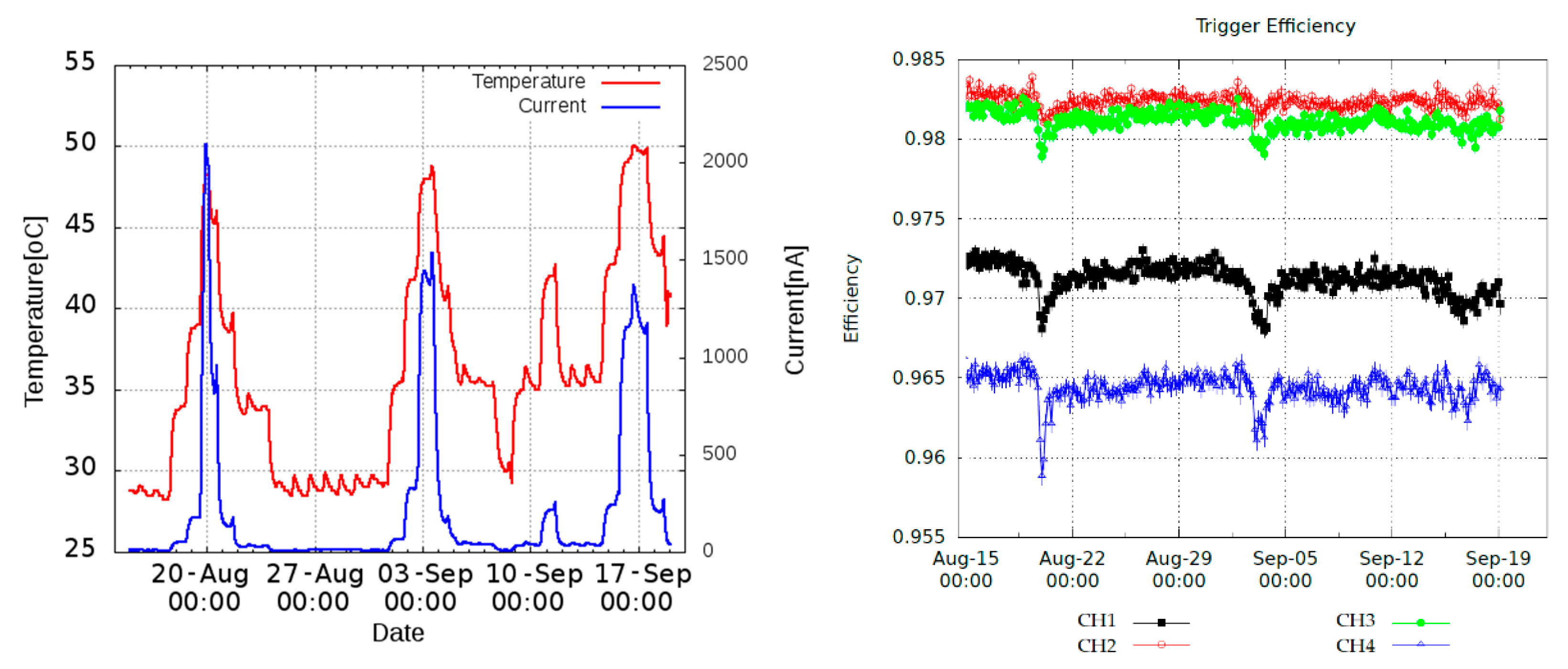
Figure 8, increases exponentially, reaching a few hundred nA at 40 °C. It is confirmed, as shown in
Figure 5, that detectors operate well even at dark currents well above 2000 nA, without apparent problems, such as noise, permanent damage or temperature runaway. Tracking efficiency is consistently high up to 50 °C.
Comparing the different cycles in
Figure 8, there is a “tempering” effect: the dark current reaches a considerably lower level at the same temperature, after few days of a cooler period. Taking the temperatures when the dark current I reached 500 nA resulted 42 °C in the first cycle, 44 °C in the second cycle and 46 °C in the third cycle. This procedure allowed us to not only qualify detectors but also to moderate the effect of the current on the chambers by applying a few heat cycles.
Table 1 shows the temperature values at 500 nA after each heat cycle.
4. Testing the Epoxy Resin Strength at Different Material Joints
During detector construction explained above, gluing is performed exclusively using epoxy resins. These adhesives can appear with various forms for example flexible or rigid, transparent or colored, and the pot life (the time where the adhesive can be used) can be different as well. Additionally, its attributes can be changed with active components. Many different materials can be joined with it, such as metal, wood, ceramic and polymer, although the strength of the bond can be different [
18,
19]. The construction of the chambers requires joining different materials (glass reinforced epoxy elements, copper layered elements, ABS-based polymer pillars), therefore it is relevant to know the behavior of the adhesive between these parts. In this section, corresponding measurement procedures and results are presented.
From the building process as presented earlier it is obvious that the inner support structure and the chamber walls—ensuring gas tightness besides mechanical stability—are the most critical for structural integrity. The former means the adhesive bond between the pillars and the copper layered base plates, the latter is the glass reinforced epoxy walls and the copper layer. For testing purposes, dedicated specimens were made which can be seen in
Figure 9. In both cases, a small rectangular piece of the baseplate (cathode) material was used, with holes. Unique aluminum holders were manufactured for the tensile meter grip to hold it, to which the baseplate specimens were screwed. The tensile test results are shown in
Figure 10.
The result of this “static” tensile test can be seen in
Table 2. These values has been used in the comparison with measurements (modal testing) and calculations below.
5. Study of Vibration Effects during Transportation
The transportation process of the detectors to the measurement site is usually a complicated activity, and may include long land- and air transport. The detectors must not suffer any damage during a standard handling process. Proper packaging includes a polymer foam material as a spacer between each detector, which reduces vibration effects (damps highest frequencies and shocks). A relevant feature is that the foam can distribute the different loads with their large area and thus not acting on a localized point. In this section a modal analysis will be performed for one completed chamber to determine the eigenfrequencies with measurement and Finite Element Method (FEM), with the aim to quantify the expected stress. After validating the simulation, a random vibration analysis will be carried out, imitating the air transport to achieve the stress field from the vibration and check if the bonded joints are sufficiently strong.
5.1. Experimental Modal Testing of a Chamber
In general, the modal testing can be used for the characterization of the vibrations and to investigate the dynamic properties of a system in the frequency domain. To build up the mathematical model of a structure, it is necessary to measure the vibration parameters (eigenfrequency, damping, mode shapes etc.). In this investigation, modal analysis will be used for a chamber to examine its vibration behavior and only the vertical direction is interesting, which is normal to the area of the chamber, denoted by z, because during the transport this is the most relevant direction.
When using a modal hammer, it is enough to excite the system in a few points, because all of the modes getting excited at the same time (except those when the hit point is a node). The measurement setup can be seen in
Figure 11.
To measure the signals of the hammer and the two accelerometers, they were connected through a compact DAQ system to a PC. The accelerometers were calibrated with a Brüel and Kjaer type 4294 exciter. To visualize, the input and output signal can be seen in
Figure 12.
After performing the Fourier transformation of every measurement, the eigenfrequencies appear as peaks.
Figure 13 shows all the measurements together. The eigenfrequencies are summarized in
Table 3.
In order to estimate the damping ratio for the FEM simulations below, one can approximate the envelope curve of the measurements, assuming that the largest amplitudes are coming from the first eigenfrequencies and defining the damping ratio with that for the system. Choosing the proper damping ratio value, the envelope curves can be plotted for the modal testing, as shown in
Figure 14.
5.2. Modal Analysis Using FEM Calculation
For the Finite element simulation, Ansys 2020 R2 student (20.2-July 2020) software was used where the materials were added with the following properties:
- -
FR-4/G10 (The base plates, the wire holder elements and the beams): ρ = 2000 [kg/m3], Ex = 20.4 [GPa], Ey = 18.4 [GPa], Ez = 15 [GPa], νx = 0.11 [-], νy = 0.09 [-], νz = 0.014 [-].
- -
ABS-based 3D printer filament (support pillars): ρ = 1250 [kg/m3], E = 1.85 [GPa]
The mass of the detector is 7 kg. In order to validate the model, the mass should not differ more than 5% (which was indeed true) and the first few eigenfrequencies should not differ more than 10%.
In the simulation structure, a modal analysis system was connected with a random vibration module to acquire the relevant information, such as eigenfrequencies. The element type was the general SOLID 186, which is a 20-node, 3DoF per node element and the degrees are the
x, y, z displacements. For the mesh, the multizone method was applied where uniform hexa domains builds up the model. The first validation of the model is to ensure independence on mesh density. The results are shown in
Table 4.
Figure 15 shows the meshed model with springs at the four corners imitating the foams.
The results from the simulation are summarized by
Table 5.
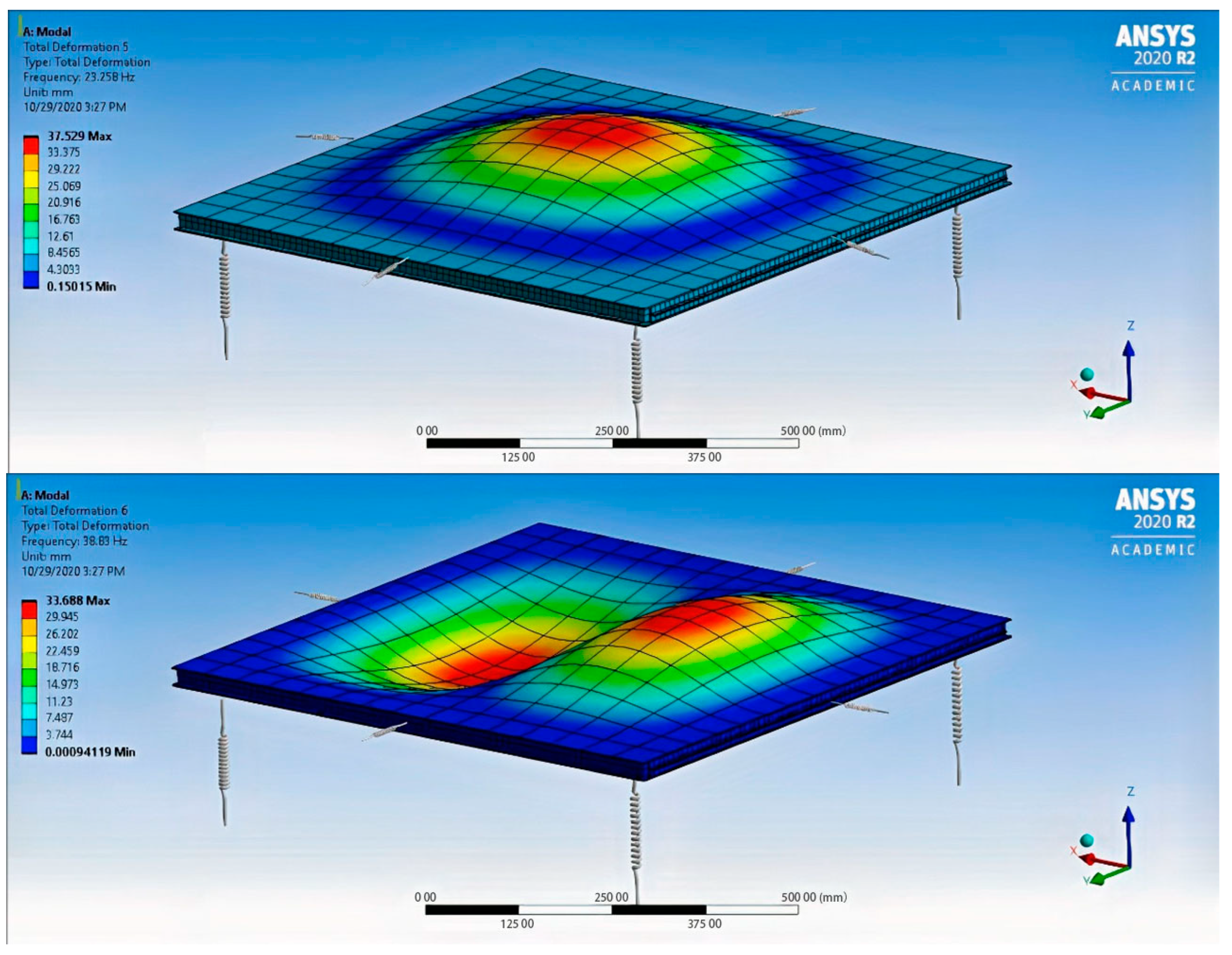
From the nice agreement between measured and simulated eigenfrequencies, one can conclude that the simulation is reasonably close to the experimental reality, and thus the model is validated. The second and the third mode shapes are shown in
Figure 16.
5.3. Random Vibration
In general, the random vibration is the most complex type of vibration where both the input and output signals characterized by random approach. D.J. Ewins [
20] specifies the method to calculate the Auto- or Power Spectral Density (PSD) or even Cross Spectral Density (CSD) for a pair of function. The PSD is useful when the resonances and harmonics are hidden in the time data and if we want to know where the energy lies. In this case the ASTM D 4169 standard [
21] was used, which defines the performance testing of shipping containers and systems. In this standard, well-detailed methods are given for uniform basis of evaluating the ability of transportability. The test plan consists of many steps, which investigating if the equipment withstands the environmental challenge. From the whole cycle, the vibration part is discussed in this paper and assumed that sudden impacts will not appear or will appear but will not damage the system during transportation. This standard refers to a test method which is discussed at ASTM D 4728 standard [
22]. It covers the random vibration testing of shipping units and determines the measurement techniques related to the performance of the container. In addition, the development and use of vibration data is discussed. For the simulation, PSD from “g” acceleration data was used where different assurance levels defined for the particular transportations (road, railway, air). To be on the safe side, assurance level 1 was used, which is a high level of test intensity and has a low probability of occurrence. The properties of this PSD for air transport can be found in
Table 6.
The lack of the fatigue test implies that a quite conservative approach must be used during the simulation to somehow connect the “static” and the “dynamic” measurements. In summary:
- ○
The test profile is the highest level of assurance, as was shown before;
- ○
The scale factor or coincidence interval is the highest (3σ or 99.73%);
- ○
The applied damping ratio is low ζ = 0.02 estimated from the modal analysis (In the literature, the value that is used in the industry for initial guessing when there is no information about the damping [
23,
24] is approximately 0.02);
- ○
Much more foams are used in the real transport box;
- ○
It is a one-time transportation to the measurement site;
- ○
Impacts are not included.
The model and the applied assurance level are shown by
Figure 17.
To emphasize again, the comparison of the “static” and the “dynamic” results are not exactly appropriate and the authors only rely on the conservative approach to connect the tensile test and the random vibration analysis.
Table 7 shows the comparison and the safety factor for each connection.
Considering that the maximal stresses from the vibrations occurs only with a very small percentage and even safety factor remains, the chambers can be transported without a problem.
6. Discussion
Muography instrumentation is derived from High Energy Physics tracking detectors, from experimental setups where an expert crew would install high performance systems, and ensure availability of around the clock maintenance and operation. For those applications which were proposed for practical muography [
1], this is very far from reality. One key step is the detector transportation, which most conveniently proceeds with standard courier, therefore anticipated mechanical stress is the same as expected at the transportation industry. The results above concluded that for the specific detector designs used particularly at the Sakurajima Muography Observatory [
25], structural integrity is secured by a broad margin. As a result of safe transportation, the world’s largest volcano-targeting tracking system could be realized and is still operational [
26]. A further step will be controlled long term endurance tests, as well as realistic impact tests.
Resistance against elevated humidity is mandatory both for underground and surface-based installations—in the former, humidity is usually constantly high at constant temperature, whereas in the latter, cooler time of the day, or even rain results in a humid environment. The present paper described a possible way to drastically improve humidity tolerance of the detectors, with the main concept of a single high voltage entry point, and complete sealing (with epoxy resin) of any external components at high voltage.
Operation at a broad temperature range, particularly at hot conditions, seemed to be challenging for most types of muography tracking systems. The results presented above were based on a controlled test in the “heat box”. After some upgrade, the heat box will also be used to simulate the effect of humidity to the system. It will be particularly interesting to investigate further the demonstrated “tempering” effect with newly constructed chambers and to later adapt a prescribed heat treatment step into the detector building and quality assurance process.
7. Conclusions
Muography detectors improved drastically during the last decade, with dedicated systems available for a broad range of applications. Experience with field installation and operation allowed developers to identify key design aspects for various technologies, which ensures a rapid, safe installation with as little crew as possible and the ability to run systems with minimal maintenance. Gaseous detectors are well suited for Muography applications due to their high efficiency, high resolution and cost effectiveness, however, traditionally these systems were more fragile than alternative detection materials (such as scintillators). This paper presented a systematic approach to improve mechanical and environmental tolerance of gaseous detectors, methods for testing and model validation, and practical construction processes. The demonstrated safe operation well above 45 °C and tolerance from vibrations during standard air freight transportation ensures predictable behavior for a broad range of applications.
Author Contributions
Software, G.H.; supervision, D.V.; writing—original draft, Á.G. and D.V.; writing—review and editing, Á.G., G.N., D.V., G.H. and G.S. All authors have read and agreed to the published version of the manuscript.
Funding
This work was supported by the Hungarian NKFIH Research Grant under No. ID OTKA-FK-135349, TKP2021-NKTA-10, János Bolyai Scholarship of the HAS and the ELKH-KT-SA-88/2021 grant. Support is acknowledged from the Joint Usage Research Project (JURP) of the University of Tokyo, Earthquake Research Institute (ERI) under project ID 2020-H-05 and the “INTENSE” H2020 MSCA RISE project under Grant Agreement No. 822185.
Acknowledgments
The authors are grateful to Gábor Szebényi and Szabolcs Pántya for the opportunity to measure in the department of polymer engineering and for Bálint Magyar for assistance and technical support with the modal analysis measurements, as well as members of the “Regard” Detector Development Group at Wigner RCP. Measurements were performed within the Vesztergombi Laboratory for High Energy Physics at Wigner RCP.
Conflicts of Interest
The authors declare no conflict of interest.
References
- Oláh, L.; Tanaka, H.K.M.; Varga, D. Muography: Exploring Earth’s Subsurface with Elementary Particles, Geophysical Monograph 270; American Geophysical Union, John Wiley & Sons, Inc.: Hoboken, NJ, USA, 2022; ISBN 9781119723028. [Google Scholar] [CrossRef]
- D’Errico, M.; Ambrosino, F.; Baccani, G.; Bonechi, L.; Bross, A.; Bongi, M.; Viliani, L. Muon radiography applied to volcanoes imaging: The MURAVES experiment at Mt. Vesuvius. J. Instrum. 2020, 15, C03014. [Google Scholar] [CrossRef]
- Presti, D.L.; Gallo, G.; Bonanno, D.L.; Bonanno, G.; Bongiovanni, D.G.; Carbone, D.; Zuccarello, L. The MEV project: Design and testing of a new highresolution telescope for muography of Etna Volcano. Nucl. Instrum. Methods Phys. Res. Sect. A 2018, 904, 195–201. [Google Scholar] [CrossRef]
- Tanaka, H.K.; Kusagaya, T.; Shinohara, H. Radiographic visualization of magma dynamics in an erupting volcano. Nat. Commun. 2014, 5, 3381. [Google Scholar] [CrossRef] [PubMed]
- Morishima, K.; Kuno, M.; Nishio, A.; Kitagawa, N.; Manabe, Y.; Moto, M.; Tayoubi, M. Discovery of a big void in Khufu’s Pyramid by observation of cosmic-ray muons. Nature 2017, 552, 386–390. [Google Scholar] [CrossRef] [PubMed]
- Morishima, K.; Nishio, A.; Moto, M.; Nakano, T.; Nakamura, M. Development of nuclear emulsion for muography. Ann. Geophys. 2017, 60, S0112. [Google Scholar] [CrossRef]
- Nishiyama, R.; Miyamoto, S.; Naganawa, N. Application of emulsion cloud chamber to cosmic-ray muon radiography. Radiat. Meas. 2015, 83, 56–58. [Google Scholar] [CrossRef]
- Bouteille, S.; Attié, D.; Baron, P.; Calvet, D.; Magnier, P.; Mandjavidze, I.; Winkler, M. A micromegas-based telescope for muon tomography: The WatTo experiment. Nucl. Instrum. Methods Phys. Res. Sect. A 2016, 834, 223–228. [Google Scholar] [CrossRef]
- Roche, I.L.; Decitre, J.B.; Gaffet, S. MUon survey tomography based on micromegas detectors for unreachable sites technology (MUST2): Overview and outlook. J. Phys. Conf. Ser. 2020, 1498, 012048. [Google Scholar] [CrossRef]
- Varga, D.; Nyitrai, G.; Hamar, G.; Oláh, L. High Efficiency Gaseous Tracking Detector for Cosmic Muon Radiography. Adv. High Energy Phys. 2016, 2016, 1962317. [Google Scholar] [CrossRef]
- Sauli, F. Principles of Operation of Multiwire Proportional and Drift Chambers; CERN: Geneva, Switzerland, 1977. [Google Scholar]
- Blum, W.; Rolandi, L. Particle Detection with Drift Chambers; Springer: Berlin/Heidelberg, Germany, 2008; ISBN 978-3-540-76683-4. [Google Scholar]
- Oláh, L.; Barnaföldi, G.G.; Hamar, G.; Melegh, H.G.; Surányi, G.; Varga, D. CCC-based muon telescope for examination of natural cave. Geosci. Instrum. Methods Data Syst. 2012, 1, 229–234. [Google Scholar] [CrossRef]
- Varga, D.; Gál, Z.; Hamar, G.; Molnár, J.S.; Oláh, É.; Pázmándi, P. Cosmic Muon Detector Using Proportional Chambers. Eur. J. Phys. 2015, 36, 6. [Google Scholar] [CrossRef]
- Nyitrai, G.; Hamar, G.; Varga, D. Toward low gas consumption of muographic tracking detectors in field applications. J. Appl. Phys. 2021, 129, 244901. [Google Scholar] [CrossRef]
- Varga, D.; Balogh, S.J.; Gera, Á.; Hamar, G.; Nyitrai, G.; Surányi, G. Construction and readout systems for gaseous muography detectors. J. Adv. Instrum. Sci. 2022, 2022, 6. [Google Scholar] [CrossRef]
- Varga, D.; Hamar, G.; Nyitrai, G.; Gera, A.; Oláh, L.; Tanaka, H.K.M. Tracking detector for high performance cosmic muon imaging. J. Instrum. 2020, 15, C05007. [Google Scholar] [CrossRef]
- Ferenc, F.; Ferenc, F.J. Handbook of Gluing Practice (A Ragasztás Kézikönyve); Műszaki Könyvkiadó: Budapest, Hungary, 1997. (In Hungarian) [Google Scholar]
- Balázs, G. Technology of Gluing (Ragasztástechnika); Műszaki Könyvkiadó: Budapest, Hungary, 1982. (In Hungarian) [Google Scholar]
- Ewins, D.J. Modal Testing: Theory and Practice; Research Studies Press: Taunton-Somerset, UK, 1989. [Google Scholar]
- ASTM D4169-16; Standard Practice for Performance Testing of Shipping Containers and Systems. ASTM International: West Conshohocken, PA, USA, 2016. Available online: www.astm.org (accessed on 1 October 2022). [CrossRef]
- ASTM D4728-17; Standard Test Method for Random Vibration Testing of Shipping Containers. ASTM International: West Conshohocken, PA, USA, 2017. Available online: www.astm.org (accessed on 1 October 2022). [CrossRef]
- Ben, B.S.; Ben, B.A.; Adarsh, K.; Vikram, K.A.; Ratnam, C. Damping measurement in composite materials under combined finite element and frequency response method. Int. J. Eng. Sci. Invention. 2013, 2, 89–97. [Google Scholar]
- Bedi, R.; Sharma, R. Damping studies on fibre-reinforced epoxy polymer concrete using Taguchi design of experiments. Int. J. Mater. Eng. Innov. 2015, 6, 42–48. [Google Scholar] [CrossRef]
- Oláh, L.; Tanaka, H.K.; Ohminato, T.; Varga, D. High-definition and low-noise muography of the Sakurajima volcano with gaseous tracking detectors. Sci. Rep. 2018, 8, 3207. [Google Scholar] [CrossRef] [PubMed]
- Oláh, L.; Tanaka, H.K.M.; Hamar, G. Muographic monitoring of hydrogeomorphic changes induced by post-eruptive lahars and erosion of Sakurajima volcano. Sci. Rep. 2021, 11, 17729. [Google Scholar] [CrossRef] [PubMed]
Figure 1.
The schematic view of three standard MWPC chamber types. The inner support structure (Support pillars and wire plane holders) becomes more and more complex as the sensitive area increases, in order to guarantee mechanical stability for field applications.
Figure 1.
The schematic view of three standard MWPC chamber types. The inner support structure (Support pillars and wire plane holders) becomes more and more complex as the sensitive area increases, in order to guarantee mechanical stability for field applications.
Figure 2.
Cross section of the MWPC detectors. The Anode/field wire plane and the Pick-up wire plane are perpendicular to each other and the wires are fixed with soldering. The readout electronics are installed on top of the chambers with proper noise reduction shielding [
10].
Figure 2.
Cross section of the MWPC detectors. The Anode/field wire plane and the Pick-up wire plane are perpendicular to each other and the wires are fixed with soldering. The readout electronics are installed on top of the chambers with proper noise reduction shielding [
10].
Figure 3.
Schematics of high voltage connection and the signal extraction (bottom of left panel) and the actual design with the ADC-card adapter. Note the gluing that covers all components on high voltage, indicated with the dashed line box on the right panel. The ADC-card acts as amplifier, and transmits the converted anode wire amplitude information to the DAQ [
14].
Figure 4.
Data Acquisition system for a muon telescope setup.
Figure 4.
Data Acquisition system for a muon telescope setup.
Figure 5.
The measurement setup for the “Heat box”. Two 50 W power resistors are responsible for internal heating. The THP sensors were placed at two different locations inside to monitor the temperature field.
Figure 5.
The measurement setup for the “Heat box”. Two 50 W power resistors are responsible for internal heating. The THP sensors were placed at two different locations inside to monitor the temperature field.
Figure 6.
The mean gain values (in arbitrary units, 30 min average) of the four chambers during 36 days of measurement period. Outside the heat cycles, the gains are technically constant.
Figure 6.
The mean gain values (in arbitrary units, 30 min average) of the four chambers during 36 days of measurement period. Outside the heat cycles, the gains are technically constant.
Figure 7.
The temperature and the current values are also plotted during the 36 days of measurement period (left). Note the dark current peaks during elevated temperatures. The trigger efficiency of the chambers was sufficiently high in the whole period (right).
Figure 7.
The temperature and the current values are also plotted during the 36 days of measurement period (left). Note the dark current peaks during elevated temperatures. The trigger efficiency of the chambers was sufficiently high in the whole period (right).
Figure 8.
The “tempering” effect. After every heat cycle the total current is getting lower at higher temperatures. This can be used to “prepare” the chambers for field applications where temperature fluctuations are high.
Figure 8.
The “tempering” effect. After every heat cycle the total current is getting lower at higher temperatures. This can be used to “prepare” the chambers for field applications where temperature fluctuations are high.
Figure 9.
The test specimens with different materials and the aluminum support.
Figure 9.
The test specimens with different materials and the aluminum support.
Figure 10.
The tensile test of the different material joints.
Figure 10.
The tensile test of the different material joints.
Figure 11.
The measurement setup with the modal hammer and the two accelerometers. Polymer foam supports were put under the chamber at the corners.
Figure 11.
The measurement setup with the modal hammer and the two accelerometers. Polymer foam supports were put under the chamber at the corners.
Figure 12.
The output signal from the accelerometer and the input signal from the hammer. In an ideal case the impact would be a Dirac-delta excitation, in reality it is finite width and must be free from contact bounce (multiple hit).
Figure 12.
The output signal from the accelerometer and the input signal from the hammer. In an ideal case the impact would be a Dirac-delta excitation, in reality it is finite width and must be free from contact bounce (multiple hit).
Figure 13.
The Fast Fourier Transformation (FFT) of the frequency response function of all measurement with the two accelerometers (A and B) in the z-direction.
Figure 13.
The Fast Fourier Transformation (FFT) of the frequency response function of all measurement with the two accelerometers (A and B) in the z-direction.
Figure 14.
The envelope curves with for measurement ID 30, using the first eigenfrequency, where e is the mathematical constant here. This roughly estimated value will be used for cross-checking against the FEM calculations.
Figure 14.
The envelope curves with for measurement ID 30, using the first eigenfrequency, where e is the mathematical constant here. This roughly estimated value will be used for cross-checking against the FEM calculations.
Figure 15.
The meshed model with the springs at the corners. Further springs were added to each side at the x-y plane to prevent the rigid body motion, the eigenfrequencies in the z direction are the same.
Figure 15.
The meshed model with the springs at the corners. Further springs were added to each side at the x-y plane to prevent the rigid body motion, the eigenfrequencies in the z direction are the same.
Figure 16.
The mode shapes related to the second (top) and the third (bottom) eigenfrequencies in the simulation.
Figure 16.
The mode shapes related to the second (top) and the third (bottom) eigenfrequencies in the simulation.
Figure 17.
The model and the applied g acceleration PSD with assurance level 1.
Figure 17.
The model and the applied g acceleration PSD with assurance level 1.
Table 1.
The temperature values after each heat cycle when the system reaches 500 nA total current and the maximum temperature. The batch 0 is related to the measurement shown in
Figure 6; the others are related to new chambers for field application (four chambers per batch). This procedure with 4 heat cycles has become a part of the construction.
| Batch | 1.Cycle | 2.Cycle | 3.Cycle | 4.Cycle | ΔT1-3 [°C] |
|---|
| T500nA | TMax | T500nA | TMax | T500nA | TMax | T500nA | TMax |
|---|
| 0. | 42 | 48 | 44 | 48.5 | 46 | 50 | - | 4 |
| 1. | 40 | 51.5 | 42 | 51 | 44 | 52 | 45.5 | 54 | 4 |
| 2. | 38 | 51 | 39.5 | 52 | 41 | 54 | 42 | 50 | 3 |
| 3. | 40 | 51 | 42 | 53 | 43 | 53 | 44 | 52 | 3 |
Table 2.
The results of the tensile test. The average force is calculated from the three different measurement. The areas of the different specimens are also shown.
Table 2.
The results of the tensile test. The average force is calculated from the three different measurement. The areas of the different specimens are also shown.
| | Average Force [N] | Tensile Strength [MPa] |
|---|
| Pillar-Baseplate (A = 22.4 mm2) | F = 128 |
σ = 5.7
|
G10-Baseplate
(A = 200 mm2) | F = 293 |
σ = 1.5
|
Table 3.
The first few eigenfrequencies of the system. Apparently the second frequency in accelerometer A was not excited, a possible reason that a node was hit. The other frequencies are in good agreement.
Table 3.
The first few eigenfrequencies of the system. Apparently the second frequency in accelerometer A was not excited, a possible reason that a node was hit. The other frequencies are in good agreement.
| Accelerometer A FFT [Hz] | Accelerometer B FFT [Hz] |
|---|
| f1 = 13.883 | f1 = 13.667 |
| - | f2 = 21.333 |
| f3 = 37.667 | f3 = 37.667 |
| f4 = 51.167 | f4 = 51.167 |
| f5 = 62.130 | f5 = 62.000 |
Table 4.
The number of elements used and the first eigenfrequencies are shown here. The error is less than 1% therefore the simulation is independent from the mesh.
Table 4.
The number of elements used and the first eigenfrequencies are shown here. The error is less than 1% therefore the simulation is independent from the mesh.
| Coarse | Ncoarse = 1784 | f1,coarse = 12.361 [Hz] |
δmesh = 0.19%
|
| Dense | Ndense = 3402 | f1,dense = 12.361 [Hz] |
Table 5.
The results from the simulation and the modal testing. It seems that the third and fourth frequencies are too close to each other and it could not be seen in the FFT.
Table 5.
The results from the simulation and the modal testing. It seems that the third and fourth frequencies are too close to each other and it could not be seen in the FFT.
| Simulation [Hz] | Modal Testing (Average) [Hz] | Error |
|---|
| f1,FEM = 12.798 | f1,Meas = 13.667 |
δ1 = 7.1%
|
| f2,FEM = 23.258 | f2,Meas = 21.333 |
δ2 = 9%
|
| f3,FEM = 38.830 | f3,4,Meas = 37.667 |
δ3,4 = 4%
|
| f4,FEM = 39.502 |
| f5,FEM = 55.214 | f5,Meas = 51.335 |
δ5 = 7.6%
|
| f6,FEM = 66.038 | f6,Meas = 62.011 |
δ6 = 6.5%
|
| f7,FEM = 74.070 | f7,Meas = 68.330 |
δ7 = 8.4%
|
Table 6.
The definition of the
g acceleration PSD with the frequency range and the amplitudes [
22].
Table 6.
The definition of the
g acceleration PSD with the frequency range and the amplitudes [
22].
| Frequency Hz | Assurance Level 1 | Assurance Level 2 | Assurance Level 3 |
|---|
| 2 | 0.0004 | 0.0002 | 0.0001 |
| 12 | 0.02 | 0.01 | 0.005 |
| 100 | 0.02 | 0.01 | 0.005 |
| 300 | 0.00002 | 0.00001 | 0.000005 |
| Overall, g rms | 1.49 | 1.05 | 0.74 |
| Duration (min) | 180 | 180 | 180 |
Table 7.
The comparison of the results from tensile test and the vibration simulation.
Table 7.
The comparison of the results from tensile test and the vibration simulation.
| Connection | Tensile Strength [MPa] | Stress from Vibration [MPa] | Safety Factor |
|---|
| G10-base plate |
σMeas = 1.47
|
σRandomvibr. = 0.15
| n = 9.8 |
| FR4-base plate |
σRandomvibr. = 0.46
| n = 3.2 |
| Pillar-base plate | σMeas = 5.7 |
σRandomvibr. = 2.12
| n = 2.7 |
| Publisher’s Note: MDPI stays neutral with regard to jurisdictional claims in published maps and institutional affiliations. |
© 2022 by the authors. Licensee MDPI, Basel, Switzerland. This article is an open access article distributed under the terms and conditions of the Creative Commons Attribution (CC BY) license (https://creativecommons.org/licenses/by/4.0/).


