1. Introduction
The response of Cherenkov calorimeters to hadrons is vastly different compared to the response to electrons. It displays strong non-linearity and rather poor energy resolution for hadrons. For instance, the CMS Hadronic Forward (HF) calorimeter is comprised of fused-silica fibers embedded in a steel absorber [
1]. It covers the forward region (3.0
5.2) where the radiation levels are measured in hundreds of Megarads. As expected, the fused-silica fibers have shown good radiation tolerance, and fast Cherenkov signals make the energy reconstruction free from signal pileup at the LHC. The HF has been working well for the measurement of tagging jets from
, where typically
50 GeV, corresponding to
500 GeV at
3.0. On the other hand, lower typical jet energies in the barrel and end-cap regions, well below 100 GeV, render the use of Cherenkov calorimetry challenging outside the forward region. We explore ways of overcoming this limitation for future experiments in this paper.
We used a Monte Carlo (MC) simulation to study the performance of a neural network (NN) to reconstruct the energy of hadronic showers in a highly granular sampling ionization calorimeter [
2]. In hadron-nucleus interactions, a large fraction of hadron energy goes into nuclear dissociation and becomes invisible. In the MC study, we viewed each hadronic shower as a 3D image with a
cm
3 pixel resolution and let the Convolutional Neural Network (CNN) estimate the invisible energy based on the features of the “image”. The CNN was trained with single charged pions of 0.5–150 GeV. The CNN trained in this way was able to estimate the invisible energy and restore the response linearity to single pions, electrons (0.5–150 GeV), and
u-quark jets (20–1000 GeV), and it surpassed the hadronic resolution attainable with a comparable dual-readout (DR) calorimeter [
3]. We used only the fast part of the signal (≤5 ns) to create these images that are mostly produced by relativistic particles and the source of Cherenkov signals.
In the following, we discuss salient characteristics of hadronic showers based on a simple MC calorimeter setup (
Section 2) and the performance of a NN in reconstructing the hadronic energy using Cherenkov signals in a highly granular fiber calorimeter (
Section 3 and
Section 4).
2. Characteristics of Hadronic Showers
Using Geant4 [
4], we simulated hadronic showers in both a solid copper absorber and a sampling calorimeter configuration with alternating plates of 17 mm copper absorber and 3 mm active material. We used the
FTFP_BERT physics list to describe hadronic interactions. The calorimeter was 1.5 m deep (8.8 interaction lengths) and
m
2 in the transverse plane. In the sampling calorimeter configuration, two active materials were chosen: silicon plates to generate the ionization and quartz plates to generate the Cherenkov signals. Neither the details of charge collection in the silicon plates and light collection in the quartz plates nor the details of the readout electronics or photo-detectors were simulated.
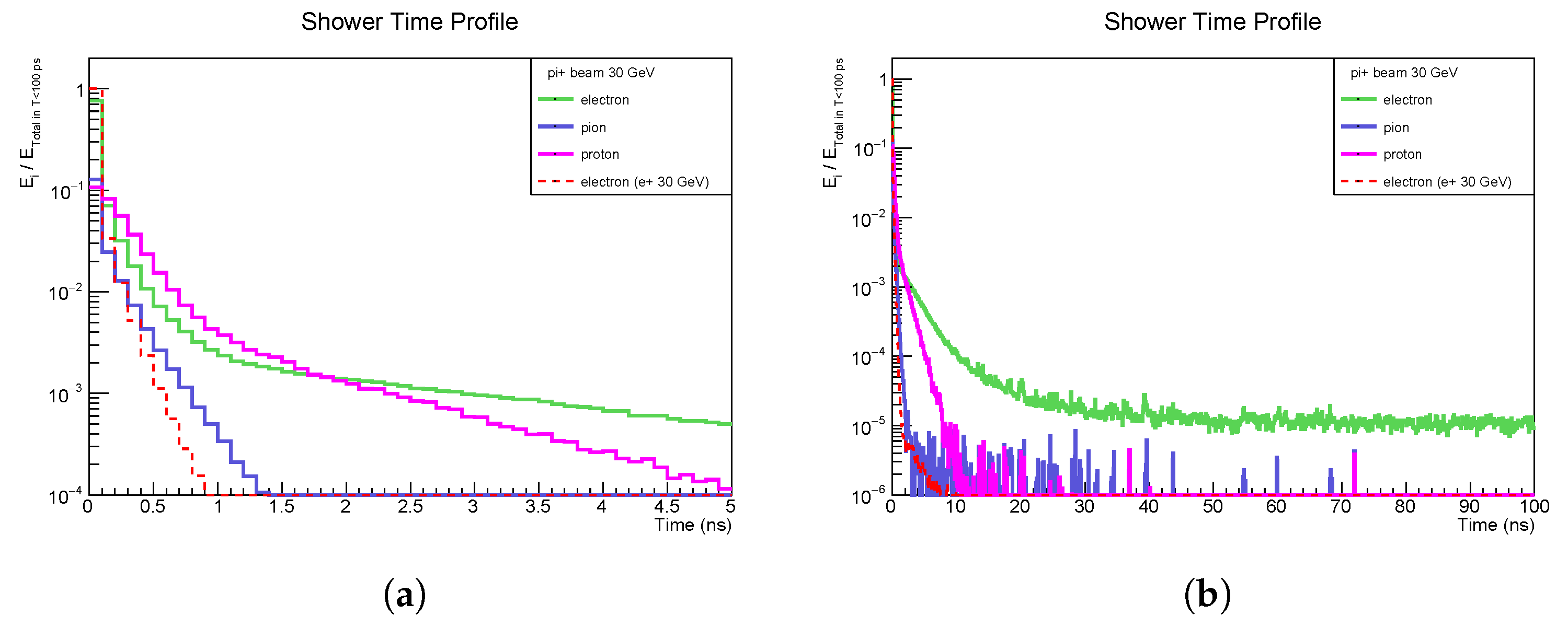
2.1. Time Structure
The time structure of the ionization signals in silicon in the sampling configuration is shown in
Figure 1. Here, the time is defined as the local calorimeter time,
, which is corrected for the travel time of all particles along the
z-axis. Three significant features emerge: (1) a very fast signal (
1 ns) due to pure electromagnetic shower and prompt pions, (2) a semi-fast signal (
5 ns) due to protons from the intra-nuclear cascade process [
5], and (3) a slow component (
100 ns and beyond) due to electrons produced by photons from neutron capture in Cu/Si. As silicon plates do not contain free protons, no slow proton signal from the neutron-proton scattering is observed. We used very fast signals (
1 ns) in this part of the analysis.
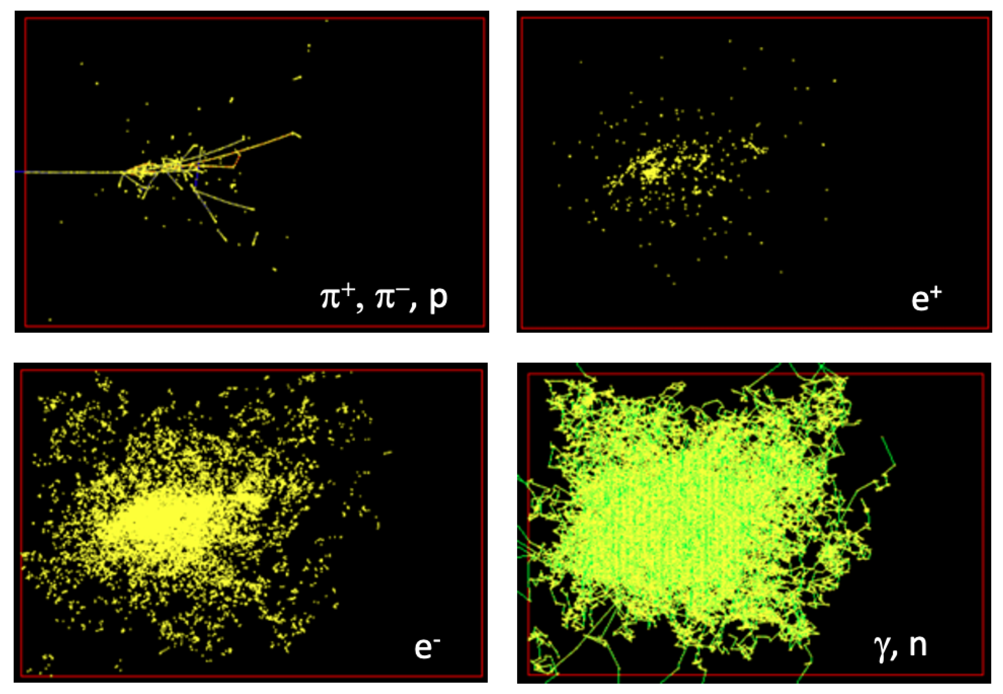
2.2. Images of Hadronic Showers
The spatial distributions of particles in the solid copper absorber from a single
are shown in
Figure 2. Pions and protons display a clear vertex-track structure. Positrons are produced in
pairs following the gamma emissions from
decays that are associated with the hadronic vertices. These pions, protons, and positrons make up the fast and semi-fast components of the shower. Neutrons and gammas are slow components and spread widely in the calorimeter. Electrons also spread widely. Some electrons are partners of positrons from
decays, and many others are from the Compton process of the widespread gammas. As seen in these images, the fast components of hadronic showers provide a distinctive vertex-track structure for the network to utilize in improved energy reconstruction.
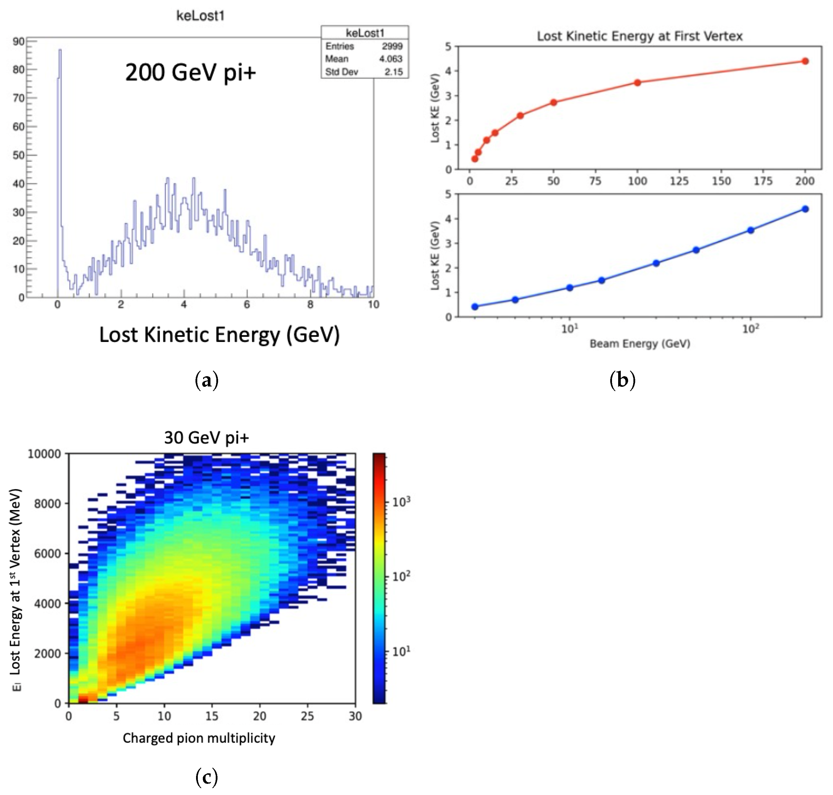
2.3. Loss of Kinetic Energy in Hadron-Nucleus Interactions
Substantial kinetic energy is lost in hadron-nucleus interactions. As shown in
Figure 3, the average energy loss is 2 or 4 GeV in
Cu interaction for 30 and 200 GeV incident pions, respectively. The multiplicity of secondary hadrons from hadron-nucleus interactions correlates with the lost kinetic energy (
Figure 3c). The CNN likely recognizes this correlation at each hadronic vertex.
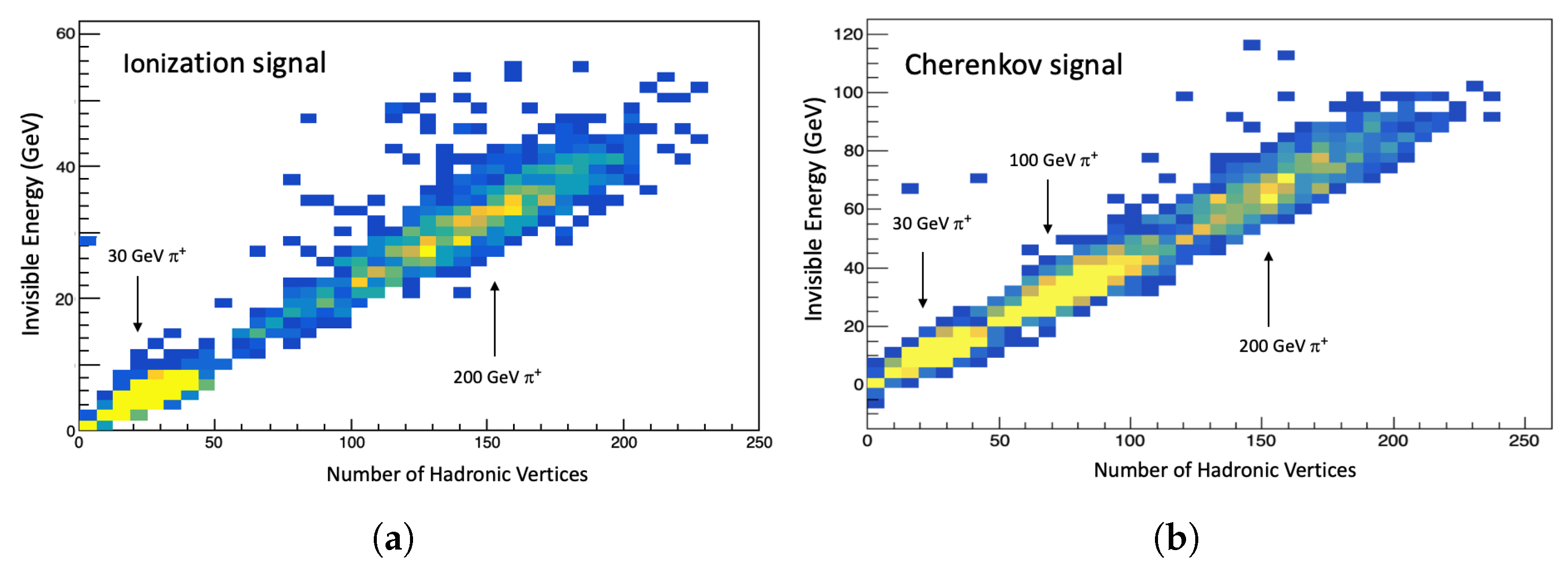
2.4. Invisible Energy in Hadronic Showers
The lost kinetic energy becomes invisible and fluctuates event by event.
Figure 4 shows the strong correlation between invisible energy and the number of hadronic vertices produced in hadron-nucleus inelastic interactions in the form of fast ionization (<5 ns) and Cherenkov signal in silicon and quartz plates. Thus, the invisible energy can be estimated with good precision if we can count the number of vertices. The “image” of a vertex is easily distinguishable: a point with outgoing tracks. We use Dynamic Graph CNN (GNN) [
6] to estimate the invisible energy in the energy reconstruction.
3. Analysis and Results Using GNN
We simulated a dual-readout fiber calorimeter (using GEANT4 with the FTFP-BERT physics list). We reconstructed the energy of hadrons using scintillation and Cherenkov signals by a simple sum of signals and the application of a GNN. The DR technique [
3] was applied and evaluated to form a benchmark as well. We used Dynamic Graph CNN (GNN) [
6], as in our previous analysis [
2]. Its new neural network module (EdgeConv) incorporates local neighborhood information because it can be stacked or recurrently applied to learn global shape properties. The GNN was trained to reproduce the incident particle energy with a large set of simulated pions in the range of 0.5–150 GeV: training (700,000), validation (100,000), and testing (300,000).
Cherenkov and scintillation fibers (1-mm diameter) were placed in a copper absorber (2-m long) with center-to-center fiber spacing of 1.5 mm. The simulated light yields were set at 100 and 400 ph/GeV for the Cherenkov and scintillation photons, respectively. Signals from multiple fibers were summed to form a transversely segmented structure. In the case of 2D, the segmentation was 1 × 1 cm2 in the transverse plane. In the case of 3D, we segmented the calorimeter into 3 × 3 cm2 in the transverse plane and utilized the time of arrival of Cherenkov photons to measure the z-position along fibers. The binning was 50 ps (about 2.5 cm), and the signal was smeared by a Gaussian distribution to evaluate the effect of timing resolution. The response of the photo-detectors and readout electronics were not simulated.
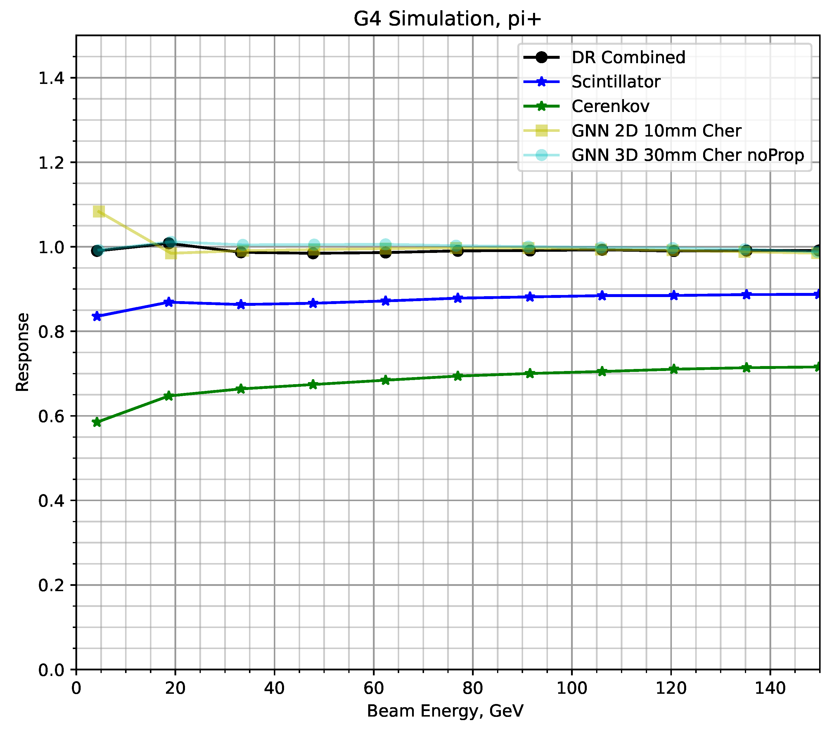
As shown in
Figure 5, the 2D segmented calorimeter response reconstructed by GNN is constant within 2% except for ∼10% deviation at the lowest energy of 4 GeV.
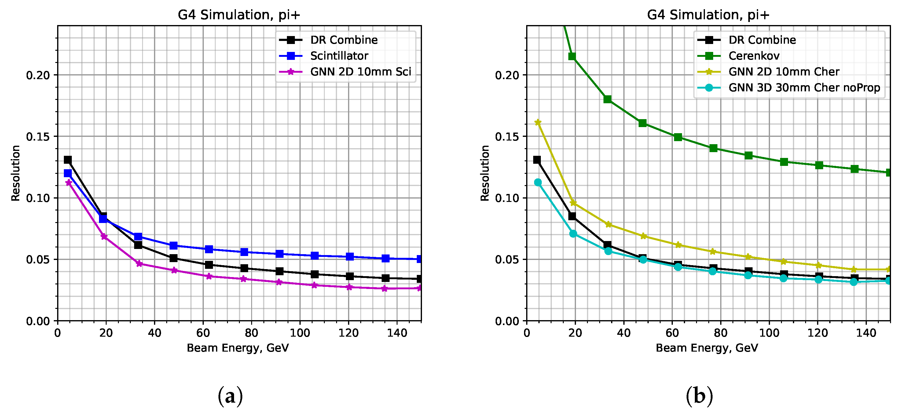
The energy resolutions obtained by the simple sum, GNN, and the dual-readout (DR) technique are shown in
Figure 6. The resolution by the DR method is shown as a reference in both plots in
Figure 6. In the scintillation case, the 2D GNN improves the resolution from 5% to 3% and surpasses the resolution by the DR method. In the Cherenkov case, the GNN methods improve the resolution from 13% to 5% with 2D and to 4% with 3D. The resolution by the 3D reconstruction is comparable to the DR resolution and better in the energy range below 20 GeV.
4. Discussion
As with our previous work [
2], the ideas presented here focused on the fast components in hadronic showers in a highly segmented calorimeter. In the approach outlined here, there is neither the traditional compensation (
) mechanism with slow neutrons nor the event-by-event evaluation of
a lá DR-based. Although further studies are clearly needed, we posit that the network effectively takes advantage of the distinctive features of the shower images, such as hadronic vertices, that result in unusually good energy resolution. The strong correlation between the invisible energy and the number of hadronic vertices observed gives us a basis to form this conjecture.
In a hadron-nucleus interaction, the total momentum is conserved. If the interaction produces several protons and neutrons in an inter-cascade process, the initial momentum gets split among protons and neutrons in addition to the prompt pions. For example, when GeV is imparted to a proton, it has a kinetic energy of 0.43 GeV, which is available to create ionization or a Cherenkov signal, while a large fraction of the initial momentum is taken away by the proton mass. The number of inelastic hadronic vertices reflects the number of protons and neutrons produced in the shower and may indicate the invisible energy due to the mass effect in the shower. The GNN is capable of recognizing the vertices in the 3D view of the shower.
4.1. A Simple Check of 2D Cherenkov Reconstruction
The 2D GNN reconstruction improved the energy resolution by more than a factor of two from the simple-sum method. To check if the 2D image of a Cherenkov signal has enough information to estimate the invisible energy and restore the beam energy, we scanned the 2D images of the Cherenkov signal and found that more activity in the 2D image implies more invisible energy. A couple of examples are shown in
Figure 7. The trend is summarized in
Figure 8. It shows a clear correlation between the number of hits in the 2D area and the invisible energy. This correlation does not depend on the incident beam energy. We believe that the GNN can easily utilize this information (simple hit counting) to estimate the invisible energy and restore the beam energy. It may use more complex information, such as the amplitude of each hit and the correlation of hits in the 2D space, to further improve the invisible energy estimation.
In the case of a 3D shower image, GNN may use its superior image recognition capability to improve the invisible energy estimation over the 2D reconstruction. The 2D images may be easily saturated by dense multi-particles in a jet, while 3D images are more tolerant to such saturation effects.
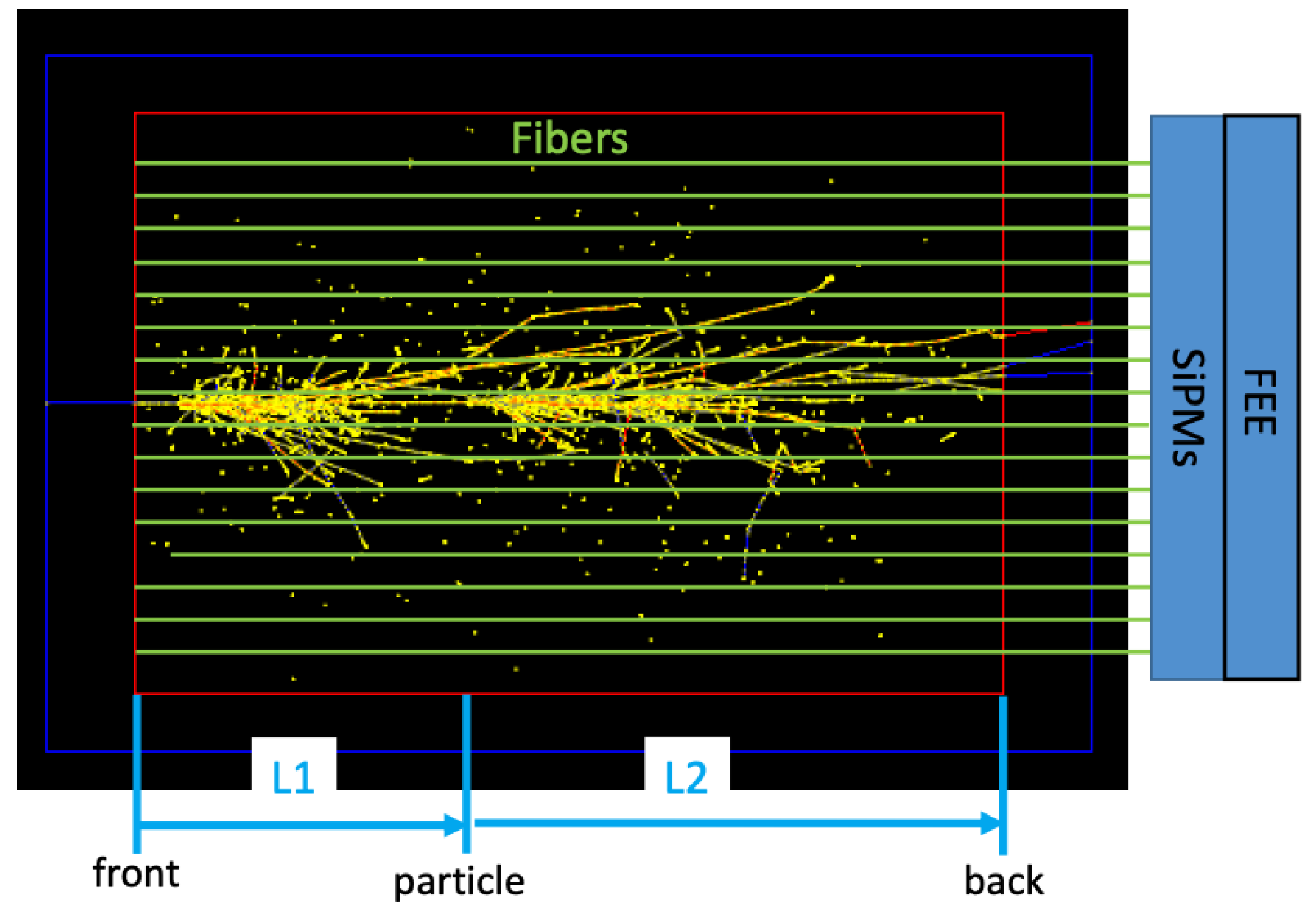
4.2. Longitudinal Segmentation by Timing
In a fiber calorimeter, the shower particles and Cherenkov photons travel approximately in the direction of the incoming particle but at different speeds. The arrival time of the photons at the downstream end of the calorimeter can be expressed as
, where
and
and
and
as shown in
Figure 9. Thus, a 2D fiber calorimeter can be turned into a 3D segmented one. The main advantages of such a device are (1) fewer channel counts than with a fully 3D segmented device, (2) protection of photo-detectors and readout electronics from radiation as they can be located behind the absorber, and (3) easier calibration without the need for depth calibration. Of course, the resolution of the timing measurement determines the effective longitudinal segmentation. The performance of the 3D GNN with various timing resolutions is summarized in
Table 1. The energy resolution with
ps matches the resolution by the DR method,
Figure 6.
Shower particles may hit the same fibers at different depths. A readout system (photo-detectors and readout electronics) requires the multi-hit capability for this kind of longitudinal segmentation. Silicon Photomultipliers (SiPMs) show excellent timing resolution for single hits, but there is currently no straightforward capability for analyzing the time structure of signals. This technology requires further R&D.
4.3. Verification of GNN Cherenkov Calorimetry
Our Monte Carlo study shows the effectiveness of neural networks in reconstructing the energy of incident hadrons from highly granular Cherenkov calorimeters. Although the result is impressive, it is based purely on a Monte Carlo simulation and needs to be verified with a prototype calorimeter in a real beam.
The effectiveness already appeared in the 2D reconstruction. We plan to modify the transverse segmentation of an existing fiber calorimeter prototype module to test the 2D reconstruction without timing information. Once we confirm the effectiveness, we move to 3D tests and more detailed simulations to optimize calorimeter designs and NN techniques for use in future experiments.
5. Conclusions
High granularity Cherenkov calorimeters combined with NN technology are poised to provide excellent performance in future high-energy experiments. The results presented here are unusually impressive and call for more detailed and systematic simulations complemented by data from a calorimeter prototype in a beam test. The combination of high granularity and powerful networks enables us to look into the mechanism of energy loss in hadron-nucleus interactions beyond the traditional views of hadronic showers. An improved understanding of the interplay between shower images and the commensurate interpretation of energy loss mechanisms will help us develop new detectors and algorithms for precision energy measurements.
Longitudinal segmentation by the timing of the Cherenkov photons will be a cost-efficient approach toward a highly segmented calorimeter and will naturally lend itself to energy reconstruction using NNs. It is clear that high-performance readout electronics and fast photo sensors are needed for this purpose.
Author Contributions
Conceptualization, methodology, N.A., C.C., J.D., A.H. and S.K.; Software, C.C., J.D. and S.K.; Validation, N.A. and C.C.; Formal Analysis, J.D., A.H. and S.K.; Data Curation, J.D. and A.H.; writing—original draft preparation, J.D., A.H. and S.K.; writing—review and editing, N.A. and C.C.; Visualization, A.H.; Project administration S.K.; Funding acquisition, N.A. All authors have read and agreed to the published version of the manuscript.
Funding
This work has been supported by the US Department of Energy, Office of Science (DE-SC0015592) and Texas Tech University, Office of the Vice President for Research and Innovation.
Data Availability Statement
Not applicable.
Acknowledgments
The authors acknowledge the High Performance Computing Center (HPCC) at Texas Tech University for providing computational resources that have contributed to the research results reported within this paper.
http://www.hpcc.ttu.edu (accessed on 15 August 2022).
Conflicts of Interest
The authors declare no conflict of interest.
References
- Abdullin, S.; Abramov, V.; Acharya, B.; Adams, M.; Akchurin, N.; Akgun, U.; Anderson, E.W.; Antchev, G.; Arcidy, M.; Ayan, S.; et al. Design, performance, and calibration of CMS forward calorimeter wedges. Eur. Phys. J. C 2008, 53, 139. [Google Scholar] [CrossRef]
- Akchurin, N.; Cowden, C.; Damgov, J.; Hussain, A.; Kunori, S. On the Use of Neural Networks for Energy Reconstruction in High-granularity Calorimeters. JINST 2021, 16, P12036. [Google Scholar] [CrossRef]
- Akchurin, N.; Carrell, K.; Hauptman, J.; Kim, H.; Paar, H.P.; Penzo, A.; Thomas, R.; Wigmans, R. Hadron and jet detection with a dual-readout calorimeter. Nucl. Instr. Meth. A 2005, 537, 537. [Google Scholar] [CrossRef]
- GEANT4 Collaboration, GEANT4—A simulation toolkit. Nucl. Instrum. Meth. A 2003, 506, 250. [CrossRef]
- Ribon, A. Hadronic Physics. Geant4 Tutorial. In Proceedings of the CERN, 22–23 January 2019; Available online: https://indico.cern.ch/event/781244/ (accessed on 15 August 2022).
- Wang, Y.; Sun, Y.; Liu, Z.; Sarma, S.E.; Bronstein, M.M.; Solomon, J.M. Dynamic Graph CNN for Learning on Point Clouds. arXiv 2018, arXiv:1801.07829. [Google Scholar] [CrossRef]
Figure 1.
Time structure of hadronic showers in a sampling calorimeter composed of 17 mm Cu absorber with 3 mm silicon layer as active material. The time is the calorimeter local time, , which is corrected for the travel time along the z-axis for all particles. (a) ( ns) is a zoomed-in view of (b) ( 100 ns).
Figure 2.
Images of shower particles for a single 30 GeV in a solid copper absorber ( cm3): Slow neutrons and s from neutron capture by nuclei spread widely and form a fuzzy image (bottom right), while fast , , and protons display a clear view of hadronic vertices and tracks (top left). The (top right) and (bottom left) are shown separately. The s arise mainly from the fast component of the shower in pairs by gammas from decays, whereas the s also arise from the slow component due to the Compton scattering of widely spread s in addition to counterparts of positions in the fast component.
Figure 3.
Loss of kinetic energy in hadron-nucleus interactions: (
a) in the 200 GeV
+Cu interaction, (
b) average energy loss in
+Cu interactions as a function of
beam energy, shown in linear and log scales, and (
c) correlation between the kinetic energy loss and the charged pion multiplicity in the 30 GeV
+Cu interactions [
2].
Figure 4.
Invisible energy the number of hadronic vertices in a sampling calorimeter: (a) with ionization signal in Cu (17 mm) + Si (3 mm) and (b) with a Cherenkov signal in Cu (17 mm) + Quartz plate (3 mm) for 30 and 200 GeV s. “Invisible energy” is defined as the difference between the beam energy and the simple sum of the ionization signal or Cherenkov signal. “Hadronic vertex” is defined as a vertex of hadron-nucleus inelastic interaction excluding neutron-nucleus interaction. The energy scale of the signals was calibrated with electrons.
Figure 5.
Response of the calorimeter to 4–150 GeV : (green) the simple sum of the Cherenkov signal, (blue) simple sum of scintillation signal, (black) dual-readout method, (yellow) GNN 2D reconstruction, and (light blue) GNN 3D reconstruction. In all cases, the calorimeter is calibrated with electrons and the signal distributions are fitted by a Gaussian distribution.
Figure 6.
Energy resolution of various reconstruction methods for 4–150 GeV beams: (a) simple sum of signal and GNN reconstruction using only the scintillation and (b) only the Cherenkov signal. The resolution by the DR technique is shown in both plots as a reference.
Figure 6.
Energy resolution of various reconstruction methods for 4–150 GeV beams: (a) simple sum of signal and GNN reconstruction using only the scintillation and (b) only the Cherenkov signal. The resolution by the DR technique is shown in both plots as a reference.
Figure 7.
A 2D () heat map of a Cherenkov signal in a 40 × 40 cm2 area: the grid size (1 × 1 cm2) corresponds to the transverse segmentation of the fiber calorimeter and the color scheme indicates the signal amplitude in . (a) An example of a large invisible energy event (beam energy 126 GeV and invisible energy 53 GeV) and (b) an example of a small invisible energy event (beam energy 127 GeV and invisible energy 1 GeV).
Figure 8.
The correlation between the number of hits in the 2D map and the invisible energy is calculated with the energy sum of a Cerenkov signal.
Figure 8.
The correlation between the number of hits in the 2D map and the invisible energy is calculated with the energy sum of a Cerenkov signal.
Figure 9.
Schematic view of a Cherenkov fiber calorimeter using timing for the longitudinal segmentation.
Figure 9.
Schematic view of a Cherenkov fiber calorimeter using timing for the longitudinal segmentation.
Table 1.
The energy resolution of the 3D GNN reconstruction with various timing resolutions for longitudinal segmentation.
Table 1.
The energy resolution of the 3D GNN reconstruction with various timing resolutions for longitudinal segmentation.
| Timing Resolution | Position Resolution | Energy Resolution |
|---|
| , ps | , cm | /E, % |
|---|
| 0 | 0.0 | 3.6 |
| 100 | 5.0 | 3.9 |
| 150 | 7.5 | 4.0 |
| 200 | 10.0 | 4.2 |
| Publisher’s Note: MDPI stays neutral with regard to jurisdictional claims in published maps and institutional affiliations. |
© 2022 by the authors. Licensee MDPI, Basel, Switzerland. This article is an open access article distributed under the terms and conditions of the Creative Commons Attribution (CC BY) license (https://creativecommons.org/licenses/by/4.0/).


