

Calorimetry in a Neutrino Observatory: The JUNO Experiment


Abstract
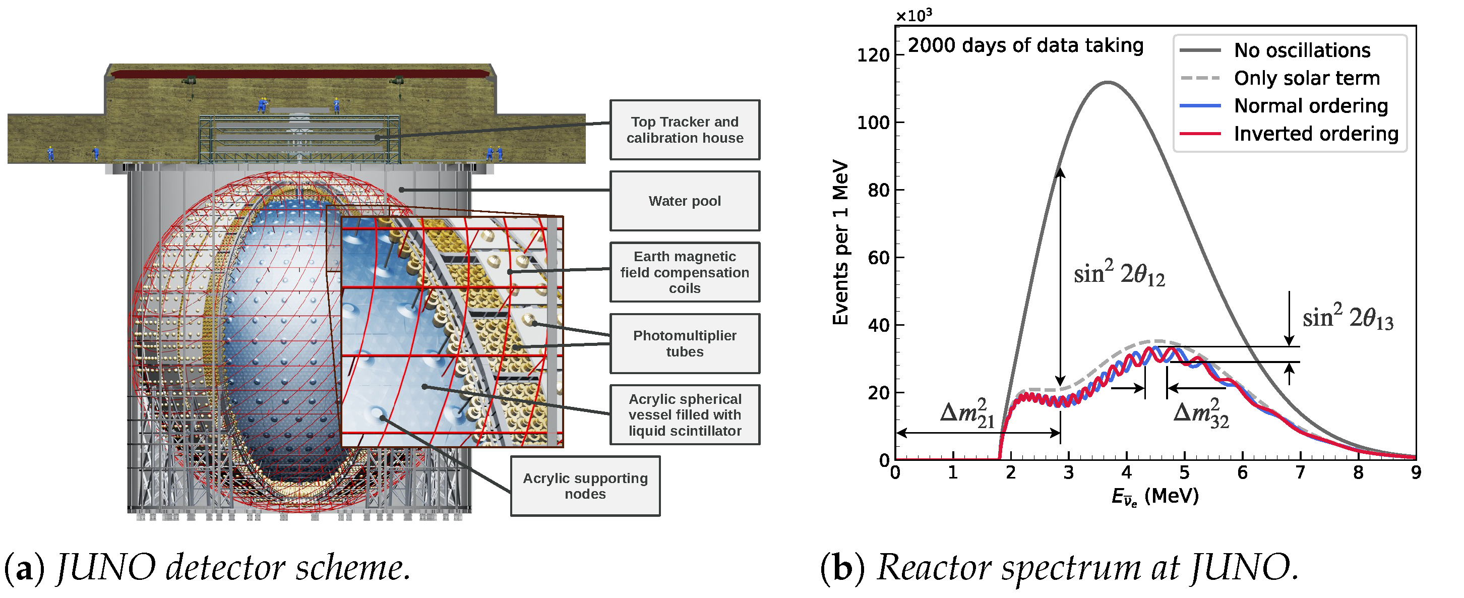
:1. Introduction: The JUNO Experiment
2. JUNO Calibration Strategy
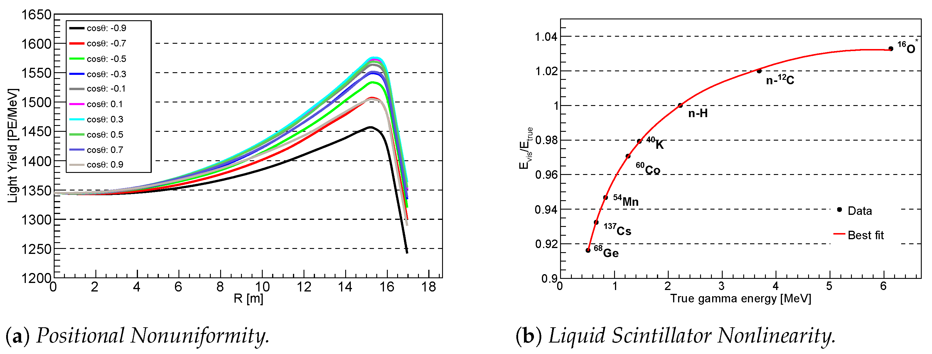
2.1. Detector Response: Liquid Scintillator Nonlinearity and Positional Nonuniformity
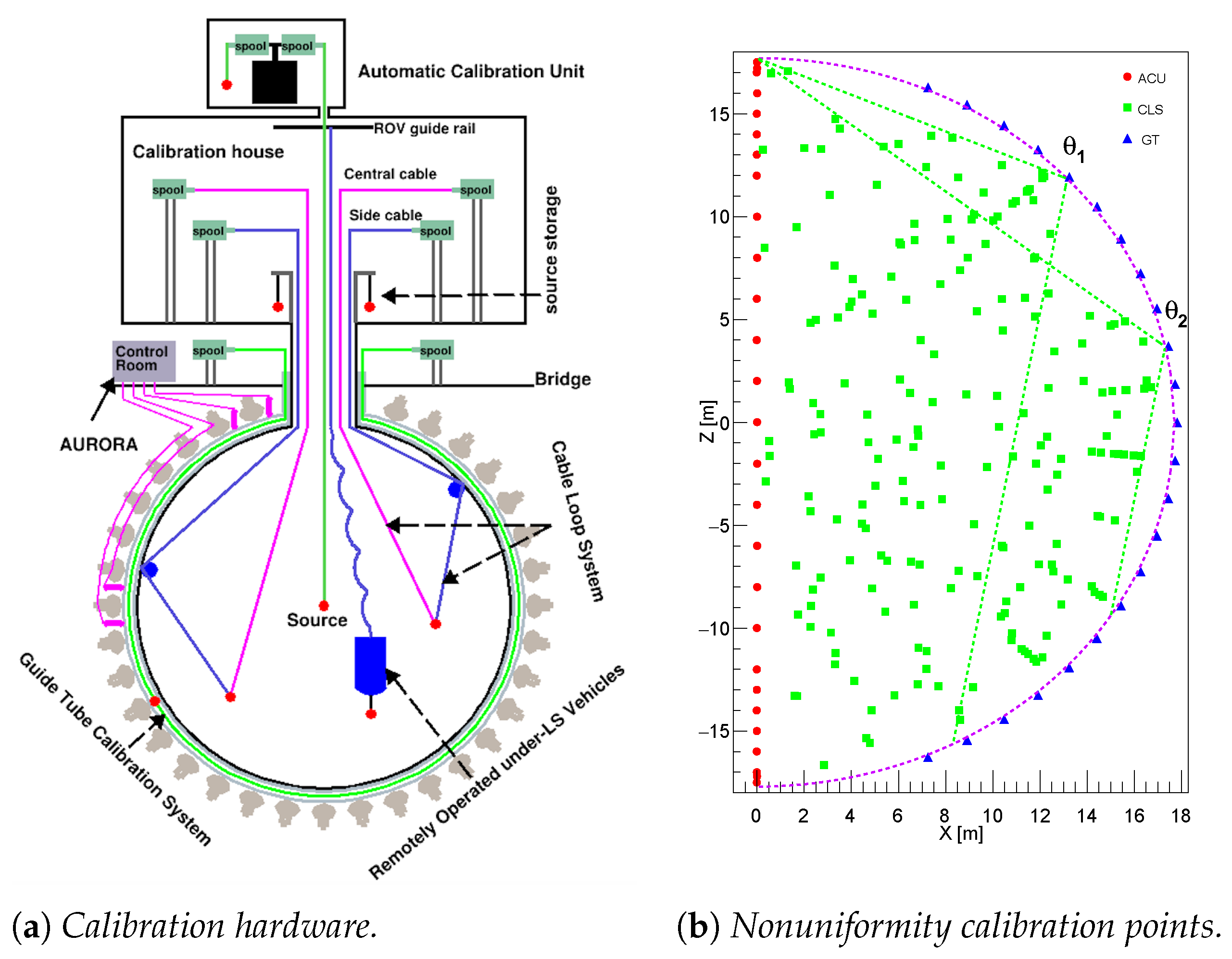
2.2. Multiple-Source and Multi-Position Calibration Campaign
2.3. Energy Resolution
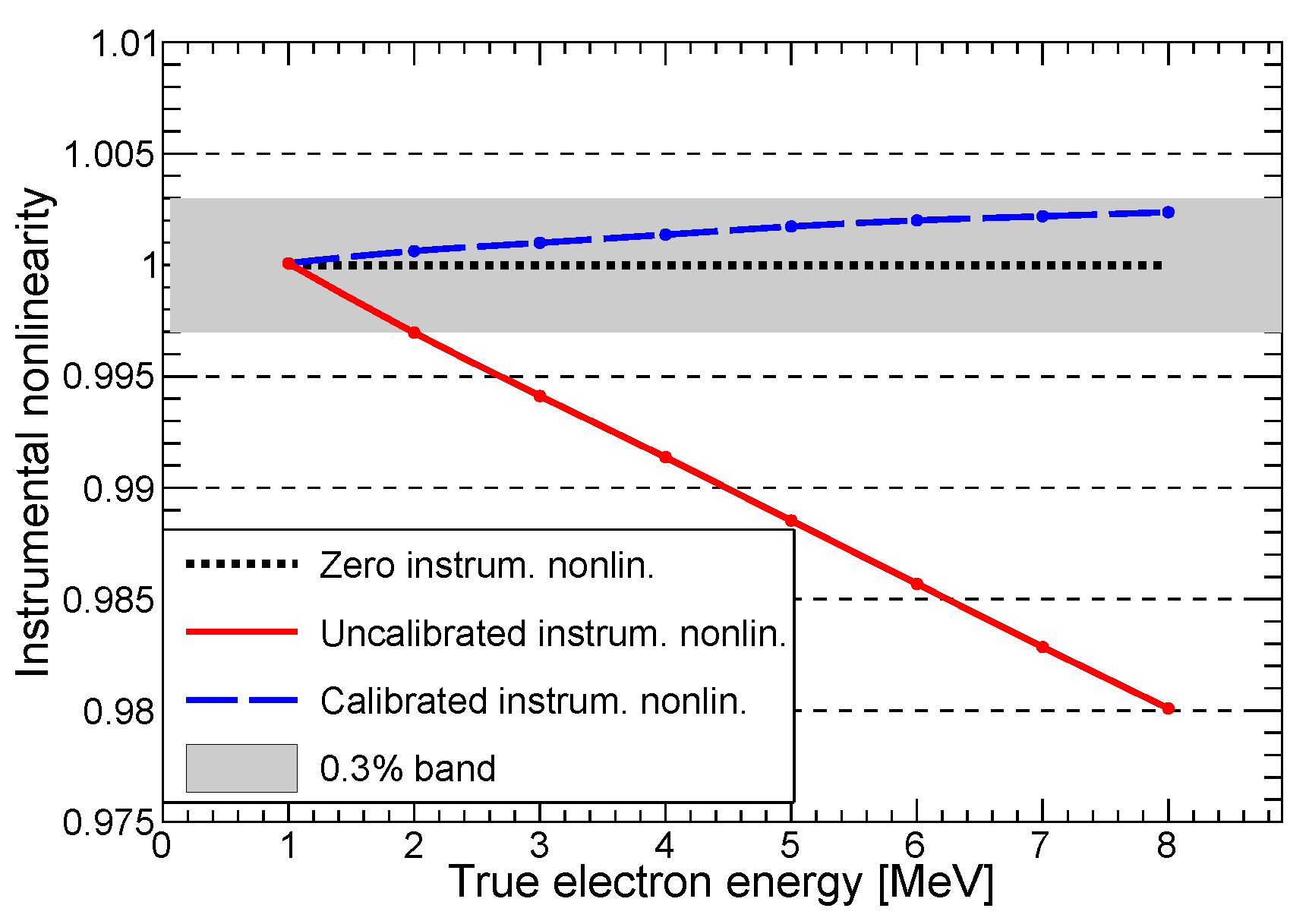
3. Dual-Calorimetry Calibration
4. Conclusions
Funding
Data Availability Statement
Conflicts of Interest
Abbreviations
| ACU | Automatic calibration unit |
| CD | Central detector |
| CLS | Cable loop system |
| DDC | Dual-calorimetry calibration |
| GT | Guide Tube |
| JUNO | Jiangmen Underground Neutrino Observatory |
| LSNL | Liquid scintillator nonlinearity |
| NU | Nonuniformity |
| PMT | Photomultiplier tube |
| QNL | Charge nonlinearity |
| ROV | Remotely operated vehicle |
References
- An, F.; An, G.; An, Q.; Antonelli, V.; Baussan, E.; Beacom, J.; Bezrukov, L.; Blyth, S.; Brugnera, R.; Buizza Avanzini, M.; et al. Neutrino Physics with JUNO. J. Phys. G Nucl. Part. Phys. 2016, 43, 30401. [Google Scholar] [CrossRef]
- The JUNO Collaboration. JUNO physics and detector. Prog. Part. Nucl. Phys. 2022, 123, 103927. [Google Scholar] [CrossRef]
- The JUNO Collaboration; Abusleme, A.; Adam, T.; Ahmad, S.; Ahmed, R.; Aiello, S.; Akram, M.; An, F.; An, G.; An, Q.; et al. Mass Testing and Characterization of 20-inch PMTs for JUNO. Eur. Phys. J. C 2022, submitted. arXiv:https://arxiv.org/abs/2205.08629. [Google Scholar]
- Workman, R.L.; Burkert, V.D.; Crede, V.; Klempt, E.; Thoma, U.; Tiator, L.; Agashe, K.; Aielli, G.; Allanach, B.C.; Amsler, C.; et al. Review of Particle Physics. Prog. Theor. Exp. Phys. 2022, 83C01. [Google Scholar]
- The JUNO Collaboration; Abusleme, A.; Adam, T.; Ahmad, S.; Ahmed, R.; Aiello, S.; Akram, M.; An, F.; An, G.; An, Q.; et al. Sub-percent Precision Measurement of Neutrino Oscillation Parameters with JUNO. Chin. Phys. C submitted. 2022, arXiv:https://arxiv.org/abs/2204.13249. [Google Scholar]
- The JUNO Collaboration; Abusleme, A.; Adam, T.; Ahmad, S.; Ahmed, R.; Aiello, S.; Akram, M.; An, F.; An, G.; An, Q.; et al. Calibration strategy of the JUNO experiment. J. High Energ. Phys. 2021, 4, 1–33. [Google Scholar] [CrossRef]
- He, M. Double Calorimetry System in JUNO. In Proceedings of the TIPP 2017, Beijing, China, 22 May 2022. [Google Scholar] [CrossRef]
- Han, Y. Dual Calorimetry for High Precision Neutrino Oscillation Measurement at JUNO Experiment. Ph.D. Thesis, Université de Paris, Paris, France, 2020. [Google Scholar]
- Lin, T.; Zou, J.; Li, W.; Deng, Z.; Fang, X.; Cao, G.; Huang, X.; You, Z.; On Behalf of the JUNO Collaboration. The Application of SNiPER to the JUNO Simulation. J. Phys. Conf. Ser. 2017, 898, 42029. [Google Scholar] [CrossRef]
- Wang, Y.G.; Cao, G.; Wen, L.; Wang, Y.F. A new optical model for photomultiplier tubes. Eur. Phys. J. C 2022, 82, 1–14. [Google Scholar] [CrossRef]
- Zhi, W. The Central Detector of JUNO. In Proceedings of the Neutrino 2022 Virtual Conference, Seoul, Korea, 30 May 2022. [Google Scholar] [CrossRef]
- An, F.P.; Balantekin, A.B.; Band, H.R.; Beriguete, W.; Bishai, M.; Blyth, S.; Rosero, R. Spectral measurement of electron antineutrino oscillation amplitude and frequency at Daya Bay. Phys. Rev. Lett. 2014, 112, 61801. [Google Scholar] [CrossRef] [PubMed] [Green Version]


Publisher’s Note: MDPI stays neutral with regard to jurisdictional claims in published maps and institutional affiliations. |
© 2022 by the author. Licensee MDPI, Basel, Switzerland. This article is an open access article distributed under the terms and conditions of the Creative Commons Attribution (CC BY) license (https://creativecommons.org/licenses/by/4.0/).
Share and Cite
Jelmini, B., on behalf of the JUNO Collaboration. Calorimetry in a Neutrino Observatory: The JUNO Experiment. Instruments 2022, 6, 26. https://doi.org/10.3390/instruments6030026
Jelmini B on behalf of the JUNO Collaboration. Calorimetry in a Neutrino Observatory: The JUNO Experiment. Instruments. 2022; 6(3):26. https://doi.org/10.3390/instruments6030026
Chicago/Turabian StyleJelmini, Beatrice on behalf of the JUNO Collaboration. 2022. "Calorimetry in a Neutrino Observatory: The JUNO Experiment" Instruments 6, no. 3: 26. https://doi.org/10.3390/instruments6030026
APA StyleJelmini, B., on behalf of the JUNO Collaboration. (2022). Calorimetry in a Neutrino Observatory: The JUNO Experiment. Instruments, 6(3), 26. https://doi.org/10.3390/instruments6030026