Performance and Calibration of the ATLAS Tile Calorimeter

Abstract

The Tile Calorimeter (TileCal) is the central hadronic calorimeter of the ATLAS experiment at the LHC. This sampling device is made of steel plates acting as absorber and scintillating tiles as active medium. The wavelength-shifting fibers collect the light from scintillators and carry it to the photomultiplier tubes (PMTs). The analogue signals from the PMTs are amplified, shaped and digitized by sampling the signal every 25 ns and stored on detector until a trigger decision is received. The TileCal front-end electronics read out the signals produced by 9852 channels, whose dynamic range covers the interval from 30 MeV to 2 TeV. Each stage of the signal propagation from scintillation light to the signal reconstruction is monitored and calibrated. During LHC Run-2, high-momentum isolated muons and isolated hadrons have been used to study and validate the electromagnetic scale and the hadronic response, respectively. The time resolution was studied with multi-jet events. Results of performance studies that address calibration, stability, energy scale, uniformity and time resolution are presented.

1. Introduction

The TileCal [1] is a hadronic calorimeter of the ATLAS experiment [2] that explores proton–proton ($pp$) and heavy ion collisions at the LHC [3] performed at the highest energies ever achieved in a laboratory. It provides essential input to the measurements of energies and directions of jets, isolated hadrons, hadronically decaying $\tau$-leptons and of the missing transverse momentum. The TileCal also contributes to the muon identification and provides information to the first level trigger.

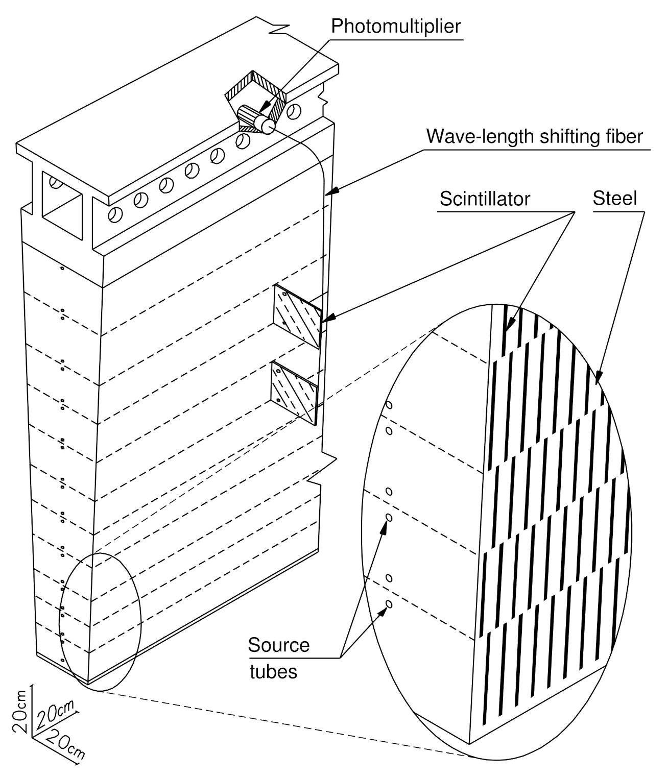
This sampling device is made of alternating layers of steel and scintillating tiles and covers the ATLAS region $\left|\eta \right|<1.7$. Mechanically, the calorimeter is divided into a central part (Long Barrel) and two Extended Barrels. Each part consists of 64 modules shown in Figure 1. The readout cells are organized into three radial layers, whose depths are 1.5, 4.1, 1.8 and 1.5, 2.6, 3.3 nuclear interaction lengths in the Long Barrel and Extended Barrels, respectively. The pseudo-projective cells are segmented in pseudorapidity ($\Delta \eta =0.1$ and $\Delta \eta =0.2$ in the outermost radial layer) and azimuth ($\Delta \varphi =2\pi /64\approx 0.1$ as defined by the module geometry). The light from scintillating tiles is collected by wavelength-shifting (WLS) fibers on both sides of each module. Each cell is readout by two photomultipliers (PMTs), whose signals are further processed by the bi-gain (high/low-gain for smaller/larger signals) readout electronics.

2. Calibration and Signal Reconstruction

The TileCal exploits three dedicated calibration systems that are briefly described below. Each system monitors different stage of the signal processing chain.

2.1. Cesium

The cesium system measures the signal induced by a ${}^{137}\mathrm{Cs}$ radioactive source that passes through all tiles. Dedicated calibration runs allow us to calibrate the optical system (tiles and WLS fibers) and PMTs. The signal is read out through dedicated slow electronics that integrate the PMT currents over 10 to 20 ms.

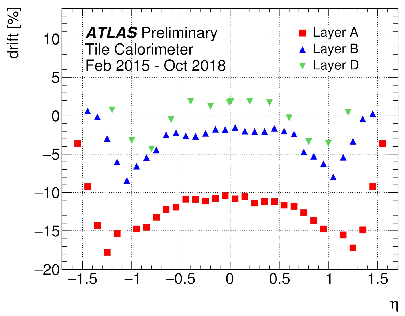
The channel response is equalized by adjusting the gain of the PMTs via their high voltage settings. The equalization is performed once at the beginning of the Run-2 data-taking period. The changes in the Cs response are tracked with calibration constants ($C_{\mathrm{Cs}}$) with a precision of about 0.3%. The Cs response evolution during Run-2 reflects the optics component degradation due to radiation dose especially pronounced in the innermost radial layer A (Figure 2) as well as the PMT gain variations discussed in Section 2.2.

2.2. Laser

Short laser pulses (The laser pulses have very similar shape to those from collision data, with a FWHM of 50 ns.) are simultaneously sent to all PMTs in order to monitor their gain and to measure possible non-linearities of their response (As more than 99.6% of all PMTs show non-linearity below 1%, no such correction is applied during the LHC Run-2.). Dedicated standalone runs are performed daily for this purpose. Laser events are also exploited during collision runs during the LHC abort gaps to track possible fast PMT gain changes as well as for monitoring the time calibration (Section 2.6).

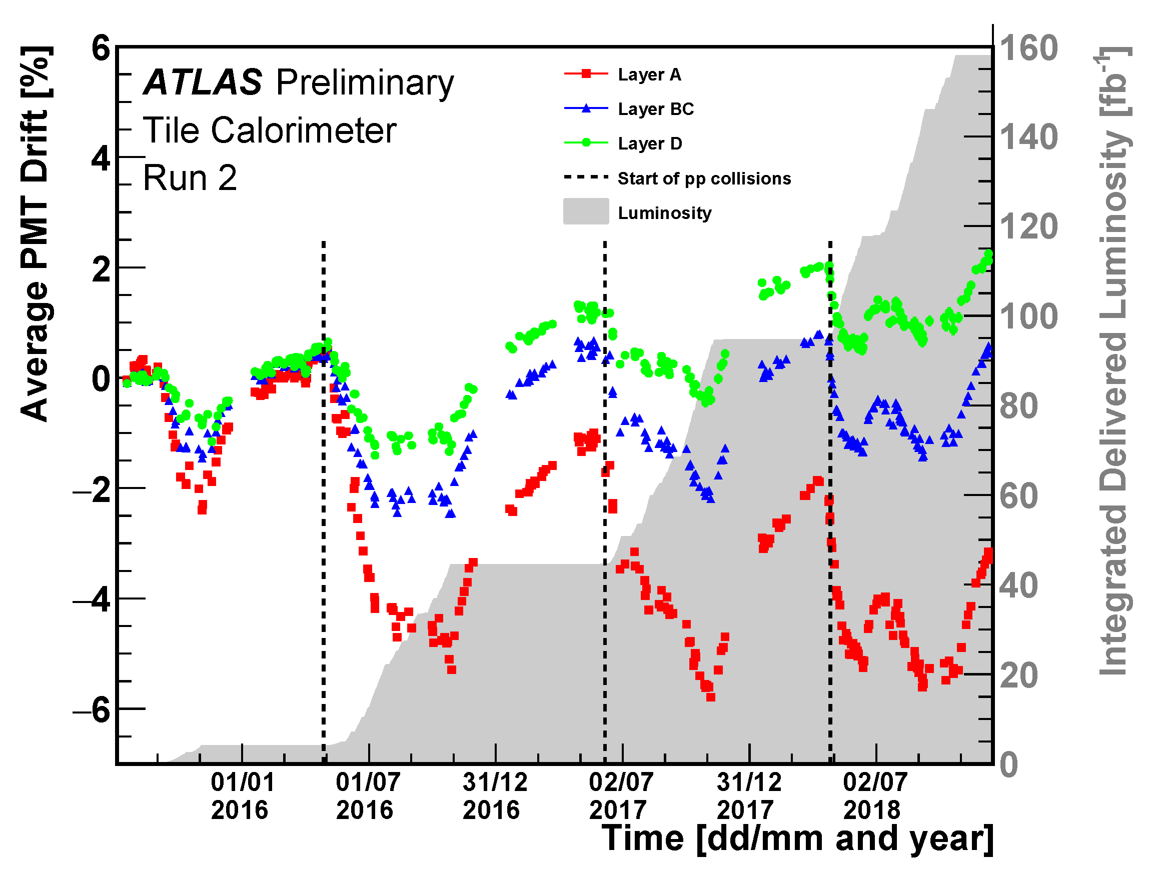
The laser calibration provides per-channel constants ($C_{\mathrm{Las}}$) that determine the PMT response relative to the last Cs calibration. The precision of the laser calibration system is at the level of 0.5%. Down-drifts are observed during collision periods, while the PMT gain recovers during the off-beam periods (Figure 3). The largest gain drifts are observed in PMTs reading cells exposed to the highest radiation dose in the innermost layer (A).

2.3. Charge Injection

A charge injection system (CIS) injects pulses of specified charge into the fast readout electronics, spanning the whole dynamic range of both gains. It provides an amplitude-to-charge conversion factor ($C_{\mathrm{CIS}}$) for every channel and gain and is also used to map non-linearities in the readout electronics.

The overall CIS precision is approximately 0.7%, and it shows very good time stability (0.05% in individual channels) over the whole Run-2.

2.4. Minimum Bias System

This system integrates the PMT response to soft inelastic interactions over many bunch-crossings. It shares the same readout path with the cesium system. As these interactions are symmetric in azimuth, this system allows for the calibration of the special cells (so-called E-cells) that are not accessible by the Cs source.

Since the minimum bias signal is proportional to the instantaneous luminosity, it is also used for the luminosity measurements [5].

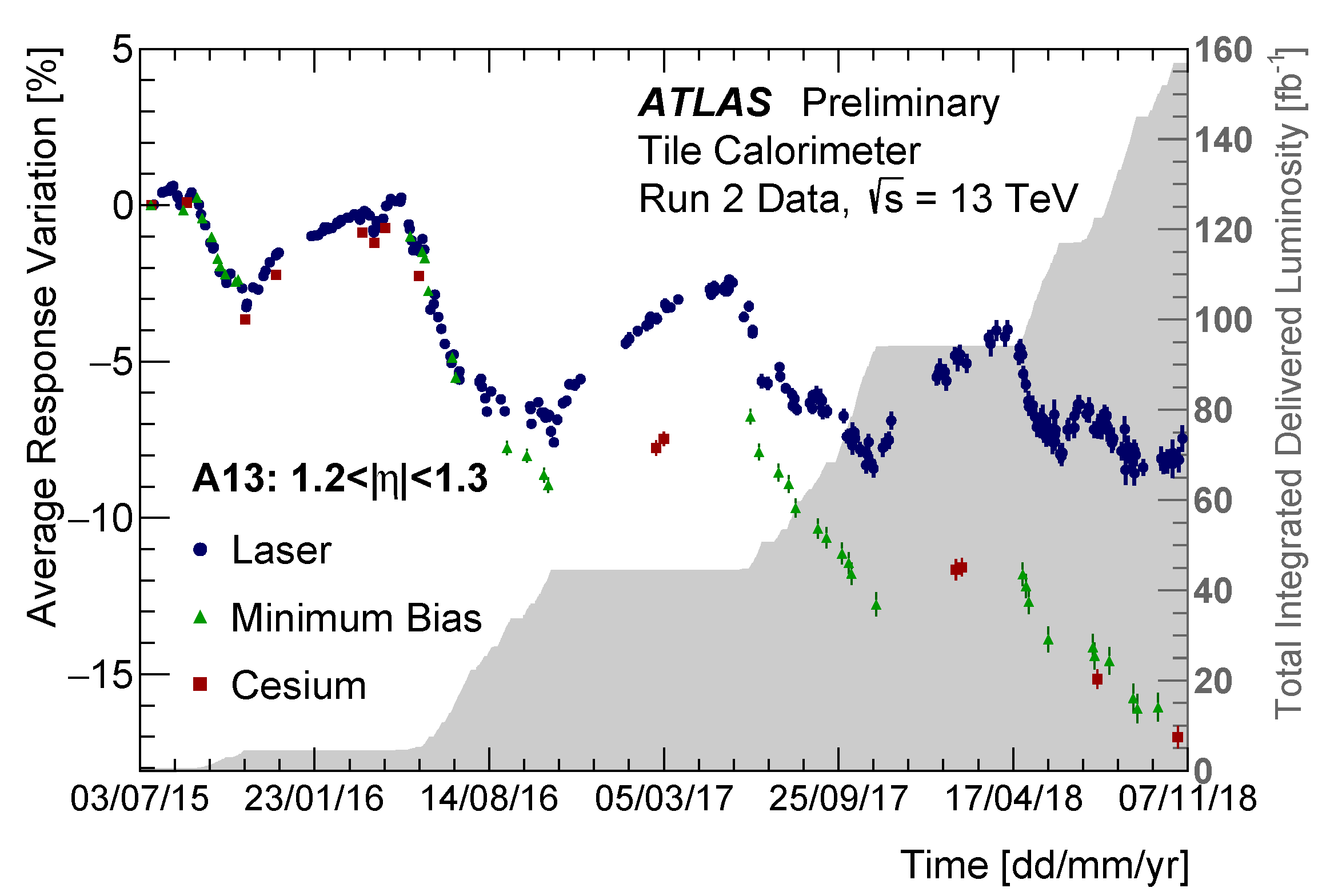
2.5. Combined Energy Calibration

Figure 4 displays the response evolution of individual calibration systems. The Cs and minimum bias results are in a very good agreement as expected. The difference between Cs and laser response is due to the optical system degradation, which amounts to approximately 10% in the most irradiated cell A13 during the LHC Run-2.

The TileCal energy in each channel is reconstructed at the electromagnetic (EM) scale using the formula

$$E\left[\mathrm{GeV}\right]=\frac{A\left[\mathrm{ADC}\mathrm{counts}\right]}{C_{\mathrm{Cs}}·C_{\mathrm{Las}}·C_{\mathrm{CIS}}[\mathrm{ADC}\mathrm{counts}/\mathrm{pC}]·C_{\mathrm{TB}}[\mathrm{pC}/\mathrm{GeV}]},$$

(1)

where A stands for the pulse amplitude reconstructed from seven consecutive samples using the Optimal Filtering (OF) algorithm [6], and $C_{\mathrm{Cs}}$, $C_{\mathrm{Las}}$ and $C_{\mathrm{CIS}}$ are the constants corresponding to the individual calibration systems. The last factor $C_{\mathrm{TB}}$ defines the EM scale and was determined in dedicated beam tests, linking the total measured charge in the calorimeter with the electron beam energy.

2.6. Time Calibration

The goal of the time calibration is to ensure that particles traveling from the ATLAS interaction point at the speed of light produce signals with a phase $t_0\approx 0$ in every channel. This feature is important for the time-of-flight measurement as well as for the proper energy reconstruction with the OF algorithm, since the OF weights depend on the phase.

The time calibration is performed on a per-channel basis with splash events (Special events are when a single LHC beam hits the collimator about 140 m upstream from the ATLAS detector. Lots of particles are produced and pass through the detector approximately parallel to the beam axis.) and initial $pp$ collisions. Only cells/channels associated to reconstructed jets are used in order to avoid bias from non-collision background. Since the mean cell time slightly depends on the deposited energy (Section 3.3), only events with channel energies between 2 and 4 GeV are selected for the calibration.

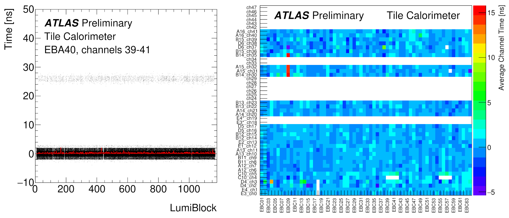
The stability of the calibration is monitored with two complementary methods, the laser events shot during the abort gaps of collision runs (Section 2.2) as well as with the physics collision data. Two examples of identified problems are shown in Figure 5. These problems are then corrected in the data used for physics analyses. The time stability is better than 1 ns.

3. Performance

The performance of the TileCal during Run-2 was checked with isolated muons and hadrons, the time resolution was addressed with jets. The improved muon identification at the first level trigger was checked with muons from Z decays.

3.1. Response to Isolated Muons

The TileCal EM scale and response uniformity was checked with isolated muons originating from the W decays. Only muon with momenta between 20 and 80 GeV are considered, since they lose their energy predominantly by ionization, hence their response scales almost linearly with the path length through the cell. The muon tracks are measured in the Inner Detector [2] and extrapolated through TileCal taking into account the detector material and magnetic field [8].

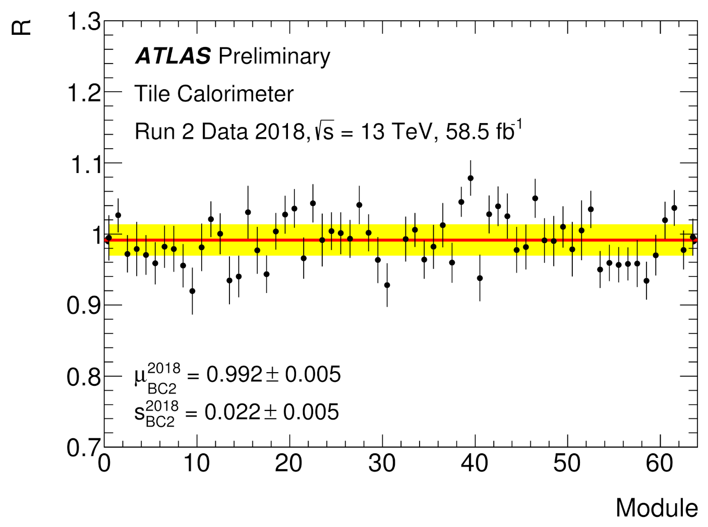
The muon response in each cell is evaluated using the ratio of deposited energy $\Delta E$ over the muon path length $\Delta x$ through that cell. As the distribution of $\Delta E/\Delta x$ is non-Gaussian, a truncated mean (Mean value of the distribution where 1% of events with the highest values are removed.) is taken as the measure of the cell response. In order to reduce the residual non-linearity of the truncated mean, the double ratio

$$R\equiv \frac{{(\Delta E/\Delta x)}_{\mathrm{data}}}{{(\Delta E/\Delta x)}_{\mathrm{MC}}}$$

(2)

is considered in the analysis. The cell response uniformity for one cell across the azimuth is shown in Figure 6. It amounts to 2.4%, and it is consistent between different cell types. Furthermore, all radial layers show a response consistent with $R=1$ within 2%.

The time stability of the response to isolated muons is addressed by comparing the double ratio R between three periods (2015 + 2016, 2017 and 2018) of Run-2. The results indicate very good stability at the level of few percents.

3.2. Response to Isolated Hadrons

The response to isolated charged hadrons was investigated with the ratio of the calorimeter energy E and associated track momentum p. This ratio was compared between data and MC simulations.

Isolated tracks are selected in the Inner Detector, and their momenta p are measured there. Only tracks with $p>2$ GeV are used. The calorimeter energy E is determined at the EM scale from calorimeter clusters associated to that isolated track (Clusters are built from calorimeter cells whose distance $\Delta R$ measured from the cluster center satisfies $\Delta R\equiv \sqrt{{({\eta }_{\mathrm{cell}}-{\eta }_{\mathrm{cluster}})}^2+{({\varphi }_{\mathrm{cell}}-{\varphi }_{\mathrm{cluster}})}^2}<0.2$.). Since this study focuses on the TileCal response, the EM calorimeter signal corresponding to that track is required to be compatible with that of a minimum ionizing particle (MIP). Muons and neutral particles are removed with further calorimeter selection criteria.

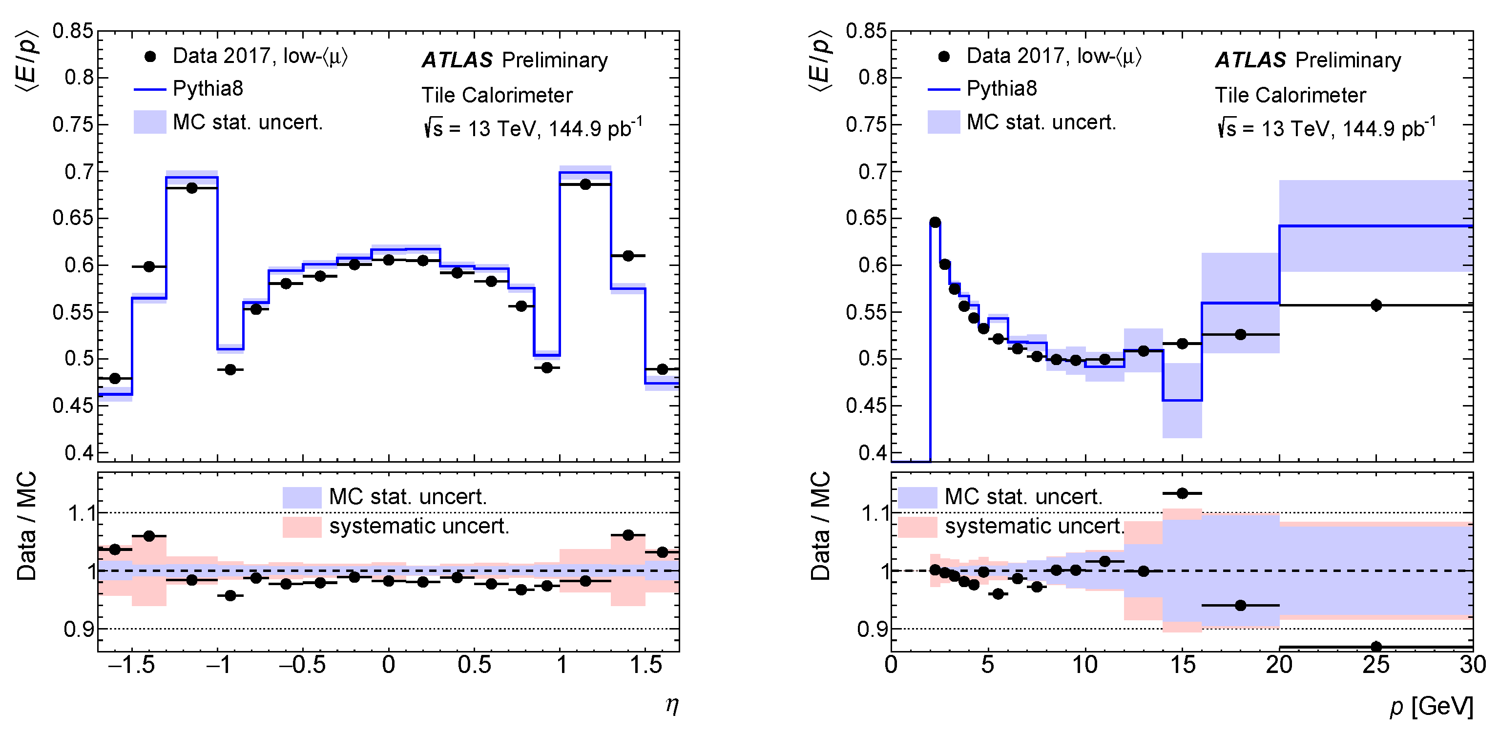
The obtained $E/p$ ratio is shown in Figure 7 as a function of pseudorapidity and track momentum for low pile-up data, i.e., where the average number of interactions per bunch-crossing is about two. A ratio $E/p<1$ is observed, reflecting the non-compensated nature of the TileCal. A good agreement between data and MC is observed for these low pile-up data. In the central region ($\left|\eta \right|<1$), the $E/p$ data/MC ratio is approximately 0.98. Similar results were reported by another ATLAS analysis [9]. A larger difference is observed in the region $\left|\eta \right|\approx 1.5$, where the data/MC ratio is affected by the so-called crack scintillators. These scintillators are designed to correct for the energy lost in the dead material between the barrel and end-cap calorimeters. Imperfections in the dead material description and a less efficient MIP-like selection in EM calorimeters in this region lead to larger discrepancies between data and MC simulations.

3.3. Time Resolution

The time performance was studied with jets. As mentioned in Section 2.6, only cells associated to the reconstructed jets are used for this purpose. Jets are required to point to the TileCal and to have a minimum transverse momentum of 20 GeV.

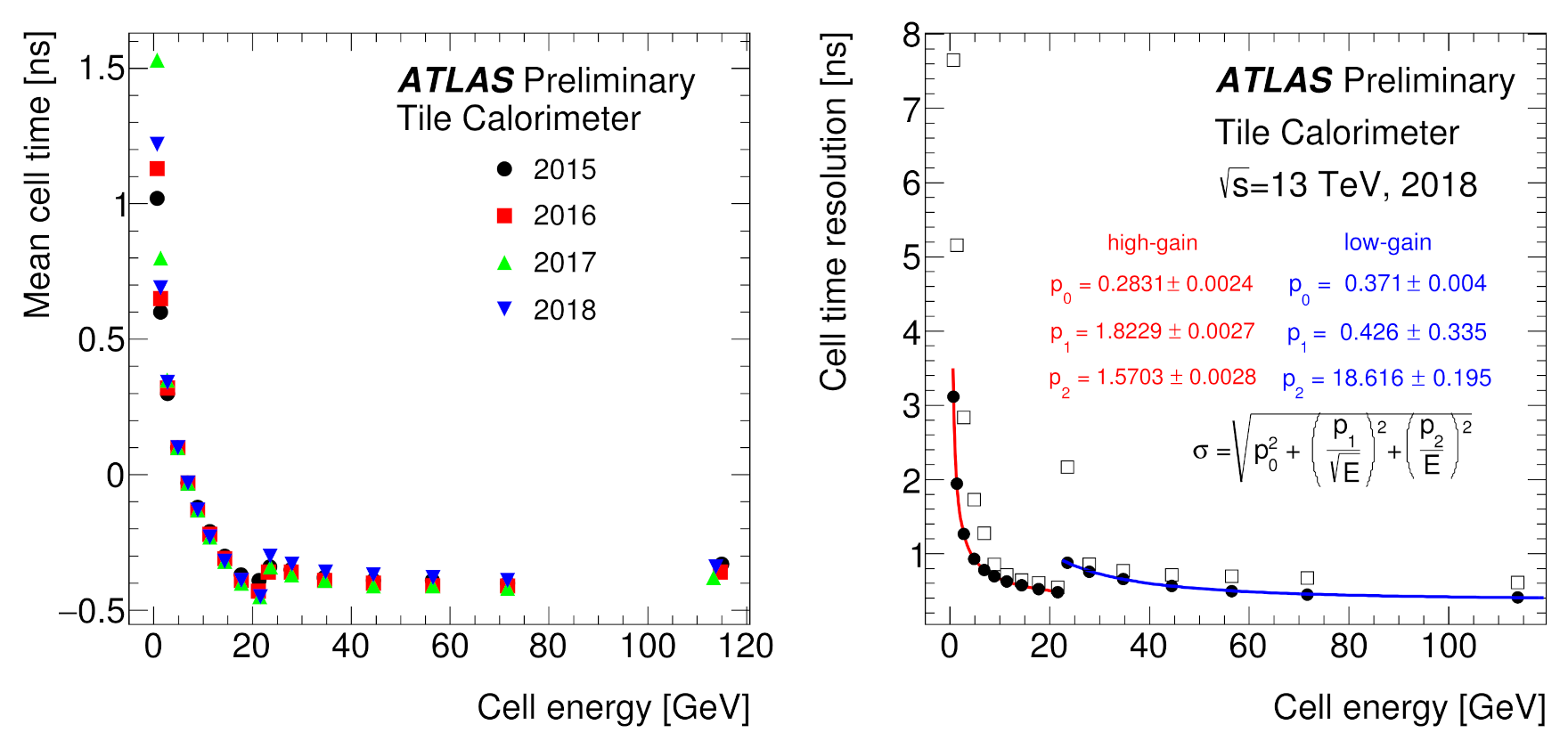
The mean cell time is stable across the four data-taking years as shown in Figure 8, left panel. It slightly decreases with the deposited energy due to neutrons and the slow hadronic component of the developed shower. The cell time resolution, determined as the Gaussian width of the corresponding time distribution, improves with energy as expected and approaches 0.4 ns at high energies (Figure 8, right). The RMS of the cell time distribution reflects the non-Gaussian tails and depends on the pile-up conditions, while the Gaussian widths are rather stable.

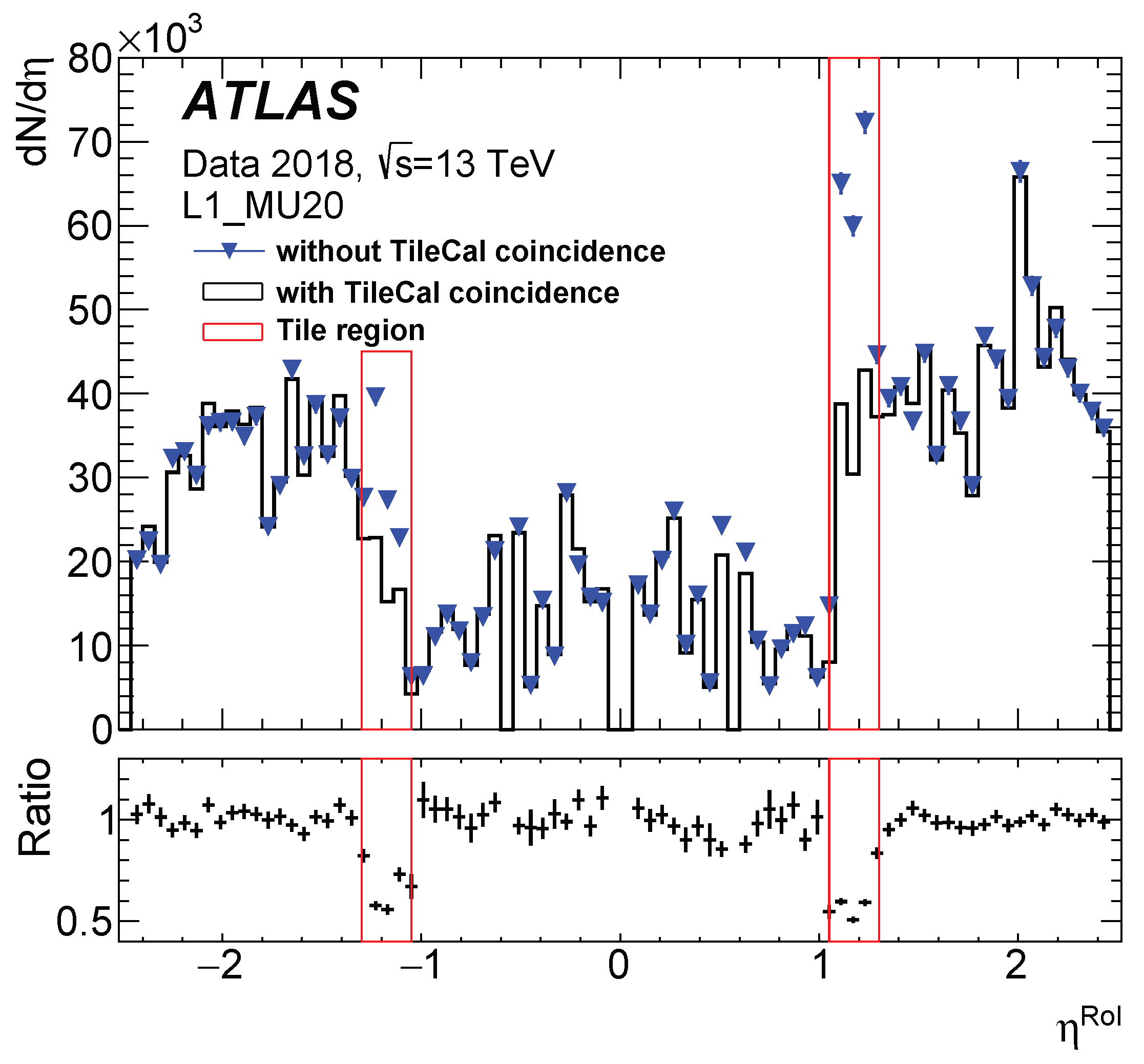
3.4. Tile-Muon Trigger

Special Tile-muon Digitizer Boards (TMDBs) have been in operation since the beginning of 2018. They provide the coincidence of signals from the outermost TileCal layer cells and the Thin Gap Chambers of the ATLAS muon system [2] in order to improve the background rejection in the first level muon trigger in the region $1.05<\left|\eta \right|<1.30$.

The pseudorapidity distribution of the reconstructed particles obtained with the Tile-muon trigger is compared to that of the first level muon trigger in Figure 9. The total trigger rate reduces by about 6%, but significant reduction is observed in the region $1.05<\left|\eta \right|<1.30$ where the TMDBs are installed. Studies with $Z\to \mu \mu$ events show that this improvement is achieved at a cost of at most 2.5% inefficiency, compatible with the expected geometrical inefficiency due to thin gaps in azimuth between the TileCal modules [10].

4. Conclusions

The ATLAS Tile Calorimeter calibration and performance during LHC Run-2 has been presented. The individual calibration systems achieve precisions better than 1%, and the combined calibration guarantees very good response stability. The time calibration exhibits a stability better than 1 ns due to the extensive monitoring.

The TileCal performance has been assessed with isolated particles and jets. The EM scale settings and the response uniformity is verified with isolated muons and single hadrons. The cell time resolution is measured with jets. It approaches 0.4 ns for energies above 100 GeV. The performance of the Tile-muon trigger, operational since 2018, has improved the background rejection in the first level muon trigger.