Article

Atmospheric and Geodesic Controls of Muon Rates: A Numerical Study for Muography Applications

by
Amélie Cohu
1,
Matias Tramontini
2,
Antoine Chevalier
3,
Jean-Christophe Ianigro
1 and
Jacques Marteau
1,*
1
Institut de Physique des 2 Infinis de Lyon (IP2I), IN2P3, CNRS, Université Lyon 1, UMR 5822, 69100 Villeurbanne, France
2
CONICET—Facultad de Ciencias Astronómicas y Geofísicas, Universidad Nacional de La Plata, La Plate 1900, Argentina
3
MUODIM, 31 rue Saint-Maximin, 69003 Lyon, France
*
Author to whom correspondence should be addressed.
Instruments 2022, 6(3), 24; https://doi.org/10.3390/instruments6030024
Submission received: 1 July 2022 / Revised: 31 July 2022 / Accepted: 2 August 2022 / Published: 4 August 2022
(This article belongs to the Special Issue Muography, Applications in Cosmic-Ray Muon Imaging)

Abstract

:
Muon tomography or muography is an innovative imaging technique using atmospheric muons. The technique is based on the detection of muons that have crossed a target and the measurement of their attenuation or deviation induced by the medium. Muon flux models are key ingredients to convert tomographic and calibration data into the 2D or 3D density maps of the target. Ideally, they should take into account all possible types of local effects, from geomagnetism to atmospheric conditions. Two approaches are commonly used: semi-empirical models or Monte Carlo simulations. The latter offers the advantage to tackle down many environmental and experimental parameters and also allows the optimization of the nearly horizontal muons flux, which remains a long-standing problem for many muography applications. The goal of this paper is to identify through a detailed simulation what kind of environmental and experimental effects may affect the muography imaging sensitivity and its monitoring performance. The results have been obtained within the CORSIKA simulation framework, which offers the possibility to tune various parameters. The paper presents the simulation’s configuration and the results obtained for the muon fluxes computed in various conditions.

1. Introduction

The Earth’s atmosphere is bombarded by charged particles called primary cosmic rays. The least energetic of them come from the Sun, while for energies between 0.1 GeV and 10 GeV, the sources are of galactic origin (mainly supernovae). Beyond that, the particles are so energetic that the sources can only be of extragalactic origin and associated with more important events in the Universe (black holes, active galactic nuclei, gamma-ray bursts, pulsars, etc.). When entering the atmosphere, these primary particles will interact with the molecules of the atmosphere, generating atmospheric showers of different particles, which are called secondary cosmic rays. Among all charged particles reaching ground level, muons are the most numerous. Their energy loss or scattering when crossing a given length of matter is exploited to reconstruct the density of the medium. The rate of high-energy cosmic ray muons as measured underground is shown to be strongly correlated with upper-air temperatures during short-term atmospheric [1,2] phenomena and with pressure [3].
Applications of atmospheric cosmic rays (CR) have grown in numbers in the last decade in the field of muography. Measurements of the muons flux attenuation (absorption muography) or deviation (scattering muography) have been successfully applied to the imaging or monitoring of large geophysical [4,5,6,7,8], archaeological [9,10,11,12,13] or industrial structures [14,15,16,17,18]; however, the measurement of the muon energy is usually not possible in small and compact field detectors, which consist of standard trackers using particle physics technologies (scintillators, resistive plate chambers, micro-mesh gaseous structures, etc). The data post-processing depends on the knowledge of the incident muon flux.
Moreover, the simulation of the muon flux follows in general two different approaches: analytical models which are derived from experimental data and cosmic rays shower generators which use Monte Carlo (MC) techniques to simulate Extended Air Showers (EAS) from the primary cosmic ray to the particles at ground level. Among the analytical models, Tang et al. [19], Shukla et al. [20], Honda et al. [21], Guan et al. [22] and Gaisser et al. [23] are often used for first estimates of the muon flux at sea level or for few elevations only. These muon generators do not require computational resources but are not customizable. Since the aim of this paper is to present results obtained with a CR generator, we propose a more extended review on the most popular ones:
  • MUPAGE [24] is a fast Monte Carlo generator of bundles of atmospheric muons for underwater/ice neutrino telescopes. It is based on parametric formulas obtained from Monte Carlo simulations of cosmic ray showers generating muons in bundle, with constraints from measurements of the muon flux with underground experiments. The range of validity extends from 1.5 km to 5.0 km of water vertical depth, and from 0° up to 85° for the zenith angle.
  • Matrix Cascade equation MCeq [25,26,27,28,29] uses numerical equation cascades to study fluxes. It is a complete Monte Carlo calculation scheme, capable of calculating neutrino, electron and muon fluxes up to 100 TeV, with a statistical accuracy of about a few percent. All particles have their own cascades of equations that represent the evolution of the energy spectrum as a function of atmospheric depth.
  • PARMA (PHITS-based Analytical Radiation Model in the Atmosphere) allows to estimate the terrestrial cosmic ray fluxes of neutrons, protons and ions, muons, electrons, positrons and photons almost anywhere on Earth and in the Earth’s atmosphere [30]. The model is based on analytical numerical functions whose parameter values are adjusted to reproduce the EAS results. The accuracy of the EAS simulation has been well verified with various experimental data.
  • CRY (Cosmic-ray Shower Library) generates showers distributions for three observation levels (sea level, 2100 m and 11,300 m) and for primary particles from 1 GeV to 10 5 GeV according to Hagmann et al. [31], and secondary particles from 10 3 to 10 5 GeV. The showers are generated in a specific area (maximum size 300 × 300   m 2 ) from pre-computed tables as explained in Hagmann et al. [32] and primary protons are produced at an altitude of 31 km in the 1976 US atmosphere [33]. In this generator, the east–west effect is not taken into account but the latitude dependence with the geomagnetic cutoff and the CR spectrum modulation are provided. It is possible to set the type of secondary particles to be studied, the altitude, the latitude, the date, the number of particles and the size of the surface of interest. The date allows to take into account the solar modulation described by Papini et al. [34]. It is possible to use pre-calculated tables from GEANT4 to take into account the configuration of the detector [35]. CRY has limitations when you investigate multi-track events in a cosmic ray experiment or identifying background events in muography.
  • CORSIKA (COsmic Ray SImulations for KAscade) [36,37] is a Monte Carlo code for simulating atmospheric particle showers initiated by high-energy cosmic ray particles. Primary particles (protons or light nuclei) are tracked in the atmosphere until they interact, decay or are absorbed. All secondary particles are explicitly followed along their trajectories and their parameters are stored when they reach an observational level.
All the models presented above have their own particularity and the choice of the fluxes generator is essential. The sensitivity of the absorption muography technique relies on the model’s accuracy, which should take into account the experimental conditions in the most realistic possible way. For instance, it has been shown in Jourde et al. [3] and Tramontini et al. [2], that atmospheric conditions strongly impact the muon flux. It is also clear that the geomagnetic field may play a significant role by deflecting charged particles towards the poles [38], which leads to a decrease in the flux at the equator and an increase at high latitudes. Furthermore the altitude of the experiment plays a role since it requires to measure the particle flux at a different stage of the cosmic shower development.
In this article, we detail the methodology and the results obtained with the CORSIKA simulation framework. In Section 2, we define the simulation main configuration parameters concerning the primary flux, the detection device, the hadronic models, the atmosphere and the geomagnetic field properties. In Section 3, we contrast the results of the simulation with analytical models, experimental data and numerical results on the effects of elevation effect, geomagnetic field and atmospheric conditions (pressure, temperature, etc.) on the muon flux are presented. Finally, in Section 4, we draw a global conclusion on the obtained tool performance.

2. Materials and Methods

2.1. Standard Use Cases

Several developments use CORSIKA for the muon fluxes simulation and for various applications. In Biallass et al. [39], they based their parametrization of the differential muon flux at ground level on a flux obtained from the air shower simulation program CORSIKA. According to Wentz et al. [40], the number of simulated particles should be normalized by taking into account the primary flux. In Mitrica et al. [41], they used this generator to determine accurately the overburden in mwe (meter water equivalent) of an underground laboratory. Pethuraj et al. [42] used CORSIKA to generate secondary particles at an experimental site where atmospheric neutrinos oscillations are studied in order to assess the long-term stability of their RPCs detectors. They studied the azimuthal dependence of the muon flux at different zenith angles and they compared they results using CORSIKA with Honda et al. [21]. For a different purpose, Kovylyaeva et al. [43] studied variations of the extra-atmospheric origin CR by introducing atmospheric effects corrections. They used CORSIKA to estimate barometric and temperature coefficients for various components of CR. Finally, Useche et al. [44] chose CORSIKA to gauge the expected cosmic ray muons flux attenuation by a structure. We use those users’ feedback to tune our CORSIKA’s options that are believed to be essential to simulate the muon flux in a specific way and we detail some of them below.

2.2. Simulation’s Configuration

We follow the muon production path from the incident primary particles to the detection level. Detailed knowledge on their properties is an important issue for the secondary particles generation.

2.2.1. Primaries at the Top of the Atmosphere

The primary cosmic ray flux is composed of several types of particles (H, He, C, O, Fe, etc). The associated fluxes are different by several orders of magnitude and the most influential flux is that of the single proton. Nevertheless, we considered different components to obtain an accurate primary flux. Several analytical models are used to describe the behavior of primary cosmic rays where the total flux J ( E ) is the sum of its various constituents and it is expressed in term of energy per nucleon (Papini et al. [34]) or per nucleus (Hörandel et al. [45], Wiebel-Sooth et al. [46]). They are our possible choices when we normalize our simulated fluxes of secondary particles with primaries spectrum. It is possible to run simulations for each primary particle type or to apply what we call the superposition principle explained by Spurio [47]. We choose the second way and we only simulated the arrival of primary protons in the atmosphere to save computation time.
Primary CR models are compared on Figure 1, their amplitudes are different depending on the energy of the primary particle. Wiebel et al. [46] seems to overestimate the flux across the full range of energy compared to Papini et al. [34]. Hörandel et al. [45] has a different behavior for energy ranges; it overestimates as well as underestimates. Figures in this paper are made using the Papini’s model, which produces an “intermediate” primary flux amplitude when compared to the others and allows to take into account the solar modulation on the expected primary CR.
  • Number of simulated showers and energy ranges
It is possible to choose the number of simulated showers per run. It is preferable (knowing the shape of the primary CR particle spectrum) to have a larger statistic for low energy particles. We choose the energy range of the primary particle to match the muon energy measurable in our tomography experiments: between 1 and 10 7 GeV. This total range is split into several parts with a defined step. The number of simulated primary particles is weighted in each bin with an empiric law for the number of showers: N = 10 9 E with E = [ 1 , 7 ] . We made this choice in order to obtain the most accurate flux possible by launching enough showers. The duration and the memory requirement of the simulations is also a factor to take into account, so we must limit ourselves to a reasonable number of showers. To be consistent, our simulated muon fluxes will be corrected by known analytical primary fluxes to cover the whole chosen spectrum.
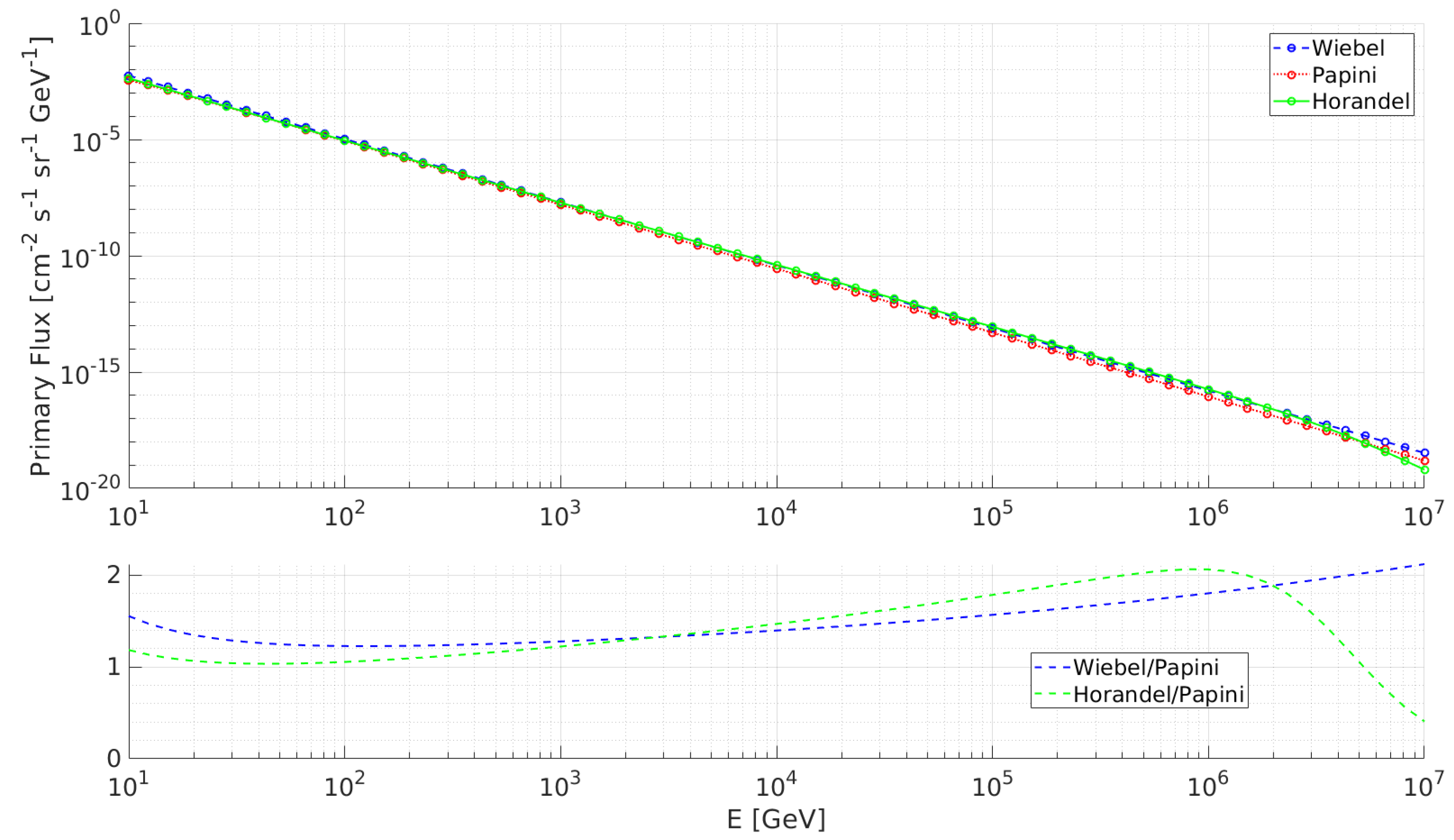
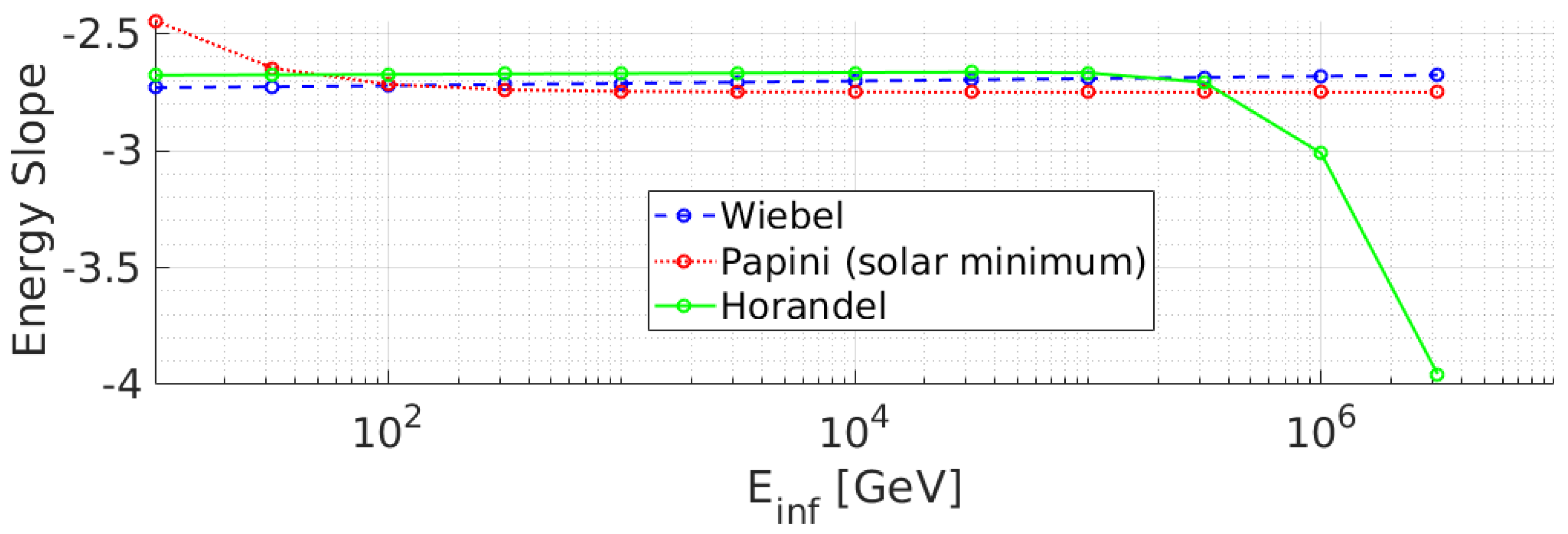
  • Slope of the primary spectra
The energy spectrum of primary CR follows a roughly exponential law: E γ . Usually γ is fixed to 2.7 for an “intermediate” energy range of primary CR spectrum according to Nesterenok et al. [48] and Pethuraj et al. [49]. In our case, γ is calculated for each energy range and run with a fit defined by an analytical model describing the primary spectrum. We selected a cosmic ray primary model based on real data fits between Papini at al. [34], Hörandel et al. [45] and Wiebel et al. [46]. Indeed, the spectrum of primaries is different from one model to another and the slope of the curve depends on the primary CR model (see Figure 2).
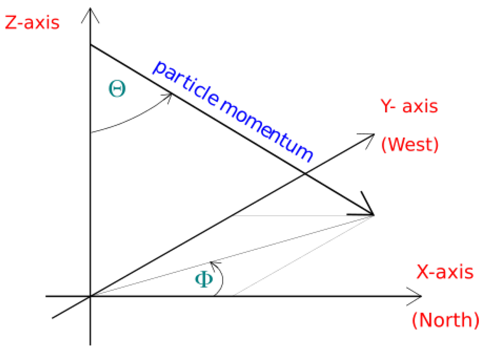
  • Particles angles trajectories
On top of energy and momentum parameters, the trajectories of particles are defined by their zenith and azimuth angles, ranging from 0° to 90° and from −180° to 180°, respectively. The coordinate system used in CORSIKA is shown in Figure 3. Furthermore, for zenith angles higher than 60° the curvature of the atmosphere is taken into account, it cannot be neglected [50].

2.2.2. Hadronic Interaction Models

When a primary particle reaches the top of the atmosphere, it undergoes “hadronic” interactions leading to the production of secondary CR and among those particles, pions and kaons decay into muons. Different types of primary particle interaction models are available on CORSIKA. We chose FLUKA for the low-energy interactions and QGSJET-II-4 for high energies, the best candidates in their energy domains for our expected accuracy and computational time.
To be more specific, FLUKA is a hadronic interaction model of low energy particles used by Usokin et al. [51], Apel et al. [52] and Heck et al. [53]. Its main strength is to allow for rapid simulation. QGSJET is a high energy hadronic interaction model. It has a high level of sophistication, approximates the data very well but is a bit slow especially because it allows few free parameters and deals with the effect of saturation by partons [54]. It is notably chosen by Tapia et al. [55] and Fedynitch et al. [26] for their simulations. In Atri et al. [56], they combine it with FLUKA.

2.2.3. Particles Energy Thresholds

To decrease the computation time and to stay compatible with the detection efficiency of our detector, we set energy thresholds values under which particles (hadrons, muons, electrons and photons) are no longer taken into account in order to simulate only the muons (or their parents) detectable by our telescopes. The choices are different in the bibliography according to the Table 1.

2.2.4. Detector Geometry and Observation Levels

CORSIKA offers three types of detector (flat, volume and vertical) associated with different angular distribution of the atmospheric shower and flux intensity [37]. For our muography detectors, the “volume” and “flat” types are preferred.
The altitude of the detector is defined by the observation levels (in cm); up to 10 levels for a simulation.

2.3. External Parameters

2.3.1. Earth’s Magnetic Field

The Earth magnetic field is created by its magnetosphere, which reduces the intensity of the high-energy flux reaching the ground. The geomagnetic field (B) modifies the spectrum of particles bombarding our atmosphere with a low-energy cutoff. The Earth’s magnetic field is able to deflect primary CR below 10 GeV near the equator and close to 1 GeV at higher latitudes. The primary CR intensity also varies with longitude because of the asymmetry of the geomagnetic axis with respect to the Earth’s rotation axis [40,49]. Those “east–west” fluxes show differences in energy intensity up to 100 GeV. This difference is more marked at high altitude than on the ground. Finally, there are significant local variations of the geomagnetic field, which affect the intensity of CR, the most famous being the South Atlantic Anomaly (SAA).
For each place, we declare the horizontal B x and vertical B z components of the Earth’s magnetic field Z (in µT), B x being the magnetic north H (see Figure 4). They are generated by the NOAA geomagnetic calculator [55]. CORSIKA computes the total magnetic field and its inclination from these two components.

2.3.2. Atmosphere Parameters

An input to CORSIKA is the state of the atmosphere in which the CR ray showers are generated. The CORSIKA atmosphere model is composed of N2, O2 and Ar with volume fractions of 78.1%, 21.0% and 0.9%, respectively. The density variation of the atmosphere with altitude is modeled by 5 layers. The state of the atmosphere is described by the density of the air at each altitude level. This parameter is calculated by converting the relative humidity into saturation vapor pressure with the Magnus formula [61]. We computed the parameters and altitudes of the layer boundaries from ERA5 data, the latest climate reanalysis produced by the ECMWF (European Centre for Medium-Range Weather Forecasts), which combines large amounts of meteorological observations with estimates made from advanced modeling and data assimilation systems [62]. The choice of ERA5 is guided by the abundance of pressure levels and the availability of data at higher altitudes.

2.3.3. Physical Validity Range

The muon rate at sea level is a logarithmic function spamming multiples order of magnitude in the energy range, and a cos ( θ ) 2 function in the angular range. The simulations encounter difficulty at the end of each of these spectrum’s range. We want to stress the fact that the estimates have well known limitations in the 70–90° angular range. They are quite limited above 10 5 GeV, where the rarity of muons is not negligible. Since the end of range in energy is not a particular issue for the muography perspectives, we consider this to be satisfactory and therefore, the chosen energy range is between 1 and 10 6 GeV.

2.4. Normalization Issues

From the CORSIKA output files we calculate the muon rate, according to the zenith angle and the muon energy, based on 10 9 E showers (see Section 2.2.1) that correspond to the validity range. Muon rates are then corrected by different factors as primary flux, geometric factor and normalization linked to the number of showers generated by the energy range.
The differential muon energy flux is written as:
Φ ( E μ , θ μ ) = F ( θ μ ) × i = 1 N p r i m j = 1 N s i m w i , j × H j ( E μ , θ μ ) N s h , j × Δ E μ
where N p r i m is the number of primary particles we want to consider in the flux calculation. N s i m is the number of simulation j. H is the histograms created as a function of the energy E and the zenith angle θ during each simulation j. Δ E μ is the width of the energy bin of the histogram. The width of the zenith angle is taking into account in F ( θ μ ) . Variations due to the azimuth angle are not taken into account here. In the interval j, we simulate N s h , j defined in Section 2.2.1.
w i , j is the normalization factor. It takes into account the contribution of the primary particle flux i [40] in the energy interval defined by the run j. We perform all our simulations with hydrogen and apply the principle of superposition: a nucleus with atomic mass number A and energy E is equivalent to a single nucleon with energy E / A . In other words, a shower initiated by a particle i containing n i nucleon, of energy n i   × E (GeV) is equivalent to n i showers of protons (of hydrogen) of energy E. The method is validated by summing the contribution of each primary particle on the muon flux and comparing it to the muon flux obtained with the superposition model. A difference is observed at low energy but since CORSIKA requires an energy higher than 80 GeV/nucleon for the primary particles other than hydrogen, the results are correct.
In order to consider the solar modulation of 4.5% (up to 100 GeV) it is recommended to use the parametrization of Papini [34] to modulate its primary particle spectrum; however, we have seen that Hörandel [45] and Wiebel [46] were two possible alternatives.
In the Papini model [34], the primary flux J is expressed in terms of energy per nucleon (in GeV/A):
w i , j = A i E j i n f E j s u p J i ( E ) d E
A i is the atomic mass of the primary particle i.
F( θ μ ) is the geometric correction factor related to the solid angle d Ω adapted to the type of detector (see [47]). For example, in the case of a flat detector: d Ω = s i n ( θ ) c o s ( θ ) d θ d ψ so:
F ( θ μ ) = 1 2 θ i n f θ s u p s i n ( θ ) c o s ( θ ) d θ
To summarize, the normalization takes into account the sampling effects of the histograms, the number of showers N s h , j generated in each simulation j, the geometric effects related to the zenith angle and the modulation of the primary i contribution over the energy range [ E i n f , j , E s u p , j ].
The integrated energy flux, for a minimum energy E m i n is obtained from the differential flux thus normalized:
Ψ ( E m i n , θ ) = E m i n Φ ( E , θ ) × d E
The discrepancy and uncertainties of muon rates are estimated using these simulations, using mean and standard deviation estimates.

3. Results

3.1. Comparison with Analytical Models

Our fluxes have been cross-checked with the analytical models listed in the Introduction. We present the results of the comparison with Tang et al. [19] regarding their integrated flux ratio I μ / I μ , 2 as a function of the muon zenith angle and for several muon energy ranges (different colors) in Figure 5. This figure presents the normalized intensity distribution when considering different energy ranges: 10–100 GeV, 100– 10 3 GeV, 10 3 10 4 GeV and the distribution for the whole energy range. The histogram of varying flux ratio values over zenith angle is meant to highlight the existence of systematic bias over the entire range of zenith values. It shows that when considering a larger energy range, the intensity ratios distribution tends to a narrow peak centered at 1.0 ± 0.2; on the whole range, the fluxes have the same intensity. Right panel shows the flux ratio for different zenith angles θ in the range 0 to 90°, when considering the same energy ranges. The models fit well on intermediate energy ranges (10– 10 2 GeV in dark blue) except at high zenith angles; however, their intensity is different at high energy ( 10 2 10 4 GeV, in light blue and green). The 1–10 GeV is range not shown: the ratio starts around 4 at 0° and increases with the zenith angle following a power law because the Tang flux is unstable at low energy and especially at high zenith angles. Our CORSIKA relative fluxes are plotted in Figure 6 only up to 2000 GeV because beyond this point our fluxes are too unstable. The part of the most energetic muons is more important than the low energetic ones at high zenith angles θ and the opposite occurs at low angles. Low-energy muons are important for calibration and high-energy muons for conducting tomography experiments; however, analytical models are known to be poorly adapted to small and large energies, because few measurements are available for their fitting equations. The CORSIKA model instead is probably more reliable over the whole energy range. Furthermore, analytical models are not extrapolated for all zenith angles and they do not take into account geodesics parameters, a limitation overcome by the CORSIKA approach.

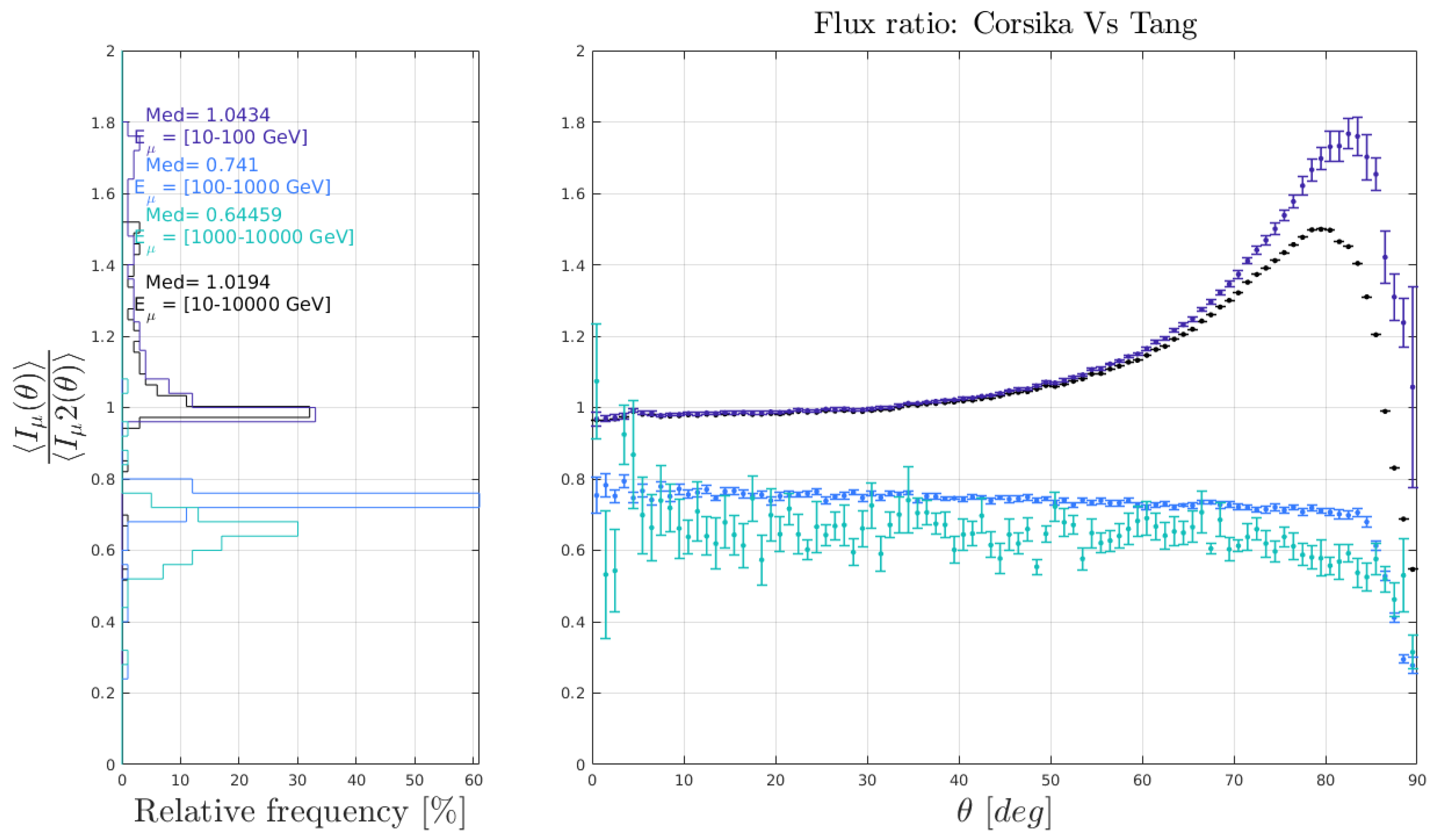
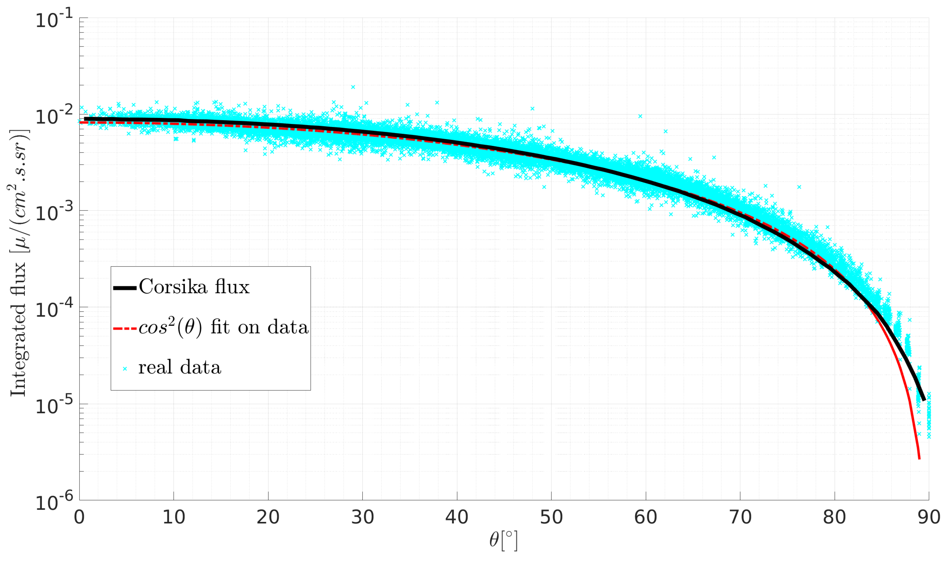
3.2. Comparison with Real Data

The best cross-checks for any simulation are the comparison to real data. Data presented here were taken in Lyon (France, latitude 45° and close to the sea level), in open sky conditions, with a 3-planes muon tracker (so-called muon telescope). We tilted the telescope progressively by step of 15° from the zenith ( θ = 0 °) to the horizontal ( θ = 90 °) directions. Multi-tracks are suppressed, electrons are partly suppressed by the multiplicity cuts on the detection planes, but there is no PID in the system. The muon flux was simulated in Lyon (France) respecting the geodesic constraints. Figure 7 displays the data/simulation comparison. Experimental points are represented with crosses in blue and the flux from CORSIKA’s simulations is represented in black. A fit was made on the real dataset with a simple c o s 2 ( θ ) at first order (in red). Despite the still pending disagreement at large zenith angles, we observed a real improvement in the data/model comparison with respect to the usual c o s 2 ( θ ) (or analytical) fit. Horizontal muons are best described by CORSIKA.

3.3. Geodesic and Atmospheric Factors

In this section, we used our CORSIKA model, validated on a large dataset to simulate muon fluxes for various particle detectionaltitude, Earth magnetic field B and atmosphere conditions. We wanted to quantify those effects on the measurable muon flux at open sky conditions. To achieve this, we varied one parameter at the time while keeping the others constant. All the results presented in this section are subject to significant uncertainty. It is statistical and increases with the energy. Indeed, we simulate much less high-energy muons and extreme-angles muons. We have limits imposed by computational time and linked to the randomness of CORSIKA. Our errors are all set to 1 σ .
For our preliminary tests we chose the city of Lyon, France (lat = 45.75° N, long = 4.75° E, B x = 22.71 µT, B z = 40.96 µT.) where we performed the open sky measurements shown in Figure 7. It is located at a medium latitude with a temperate climate. Then, we have used the parameters of Dallol, Ethiopia (lat = 14.14° N, long = 40.18° E, B x = 36.2752 µT, B z = 10.1924 µT where the hottest temperatures on Earth have been recorded. Oimiakon, Russia (lat = 69.18° N, long = 141.6° E, B x = 9.9943 µT, B z = 58.5077 µT is a plateau where the coldest temperatures in the northern hemisphere have been recorded. These two places were chosen to study extreme weather effects.

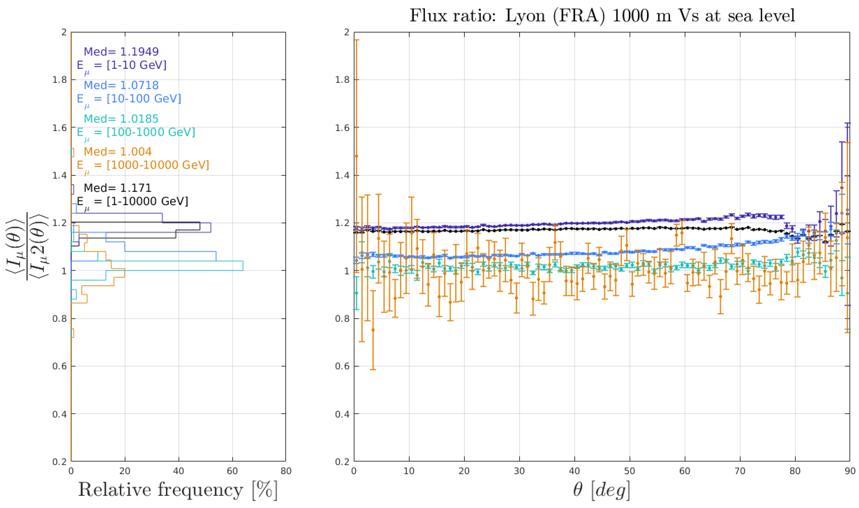
3.3.1. Altitude Effects

The altitude of the experiment plays an important role as it involves measuring the particle flux at a different stage of the cosmic shower development. We compared the muon flux in Lyon, France at 1000 m with the muon flux at sea level. Figure 8 presents the normalized intensity distribution when considering different energy ranges: 1–10 GeV, 10–100 GeV, 100– 10 3 GeV, 10 3 10 4 GeV and the distribution for the whole energy range. The histogram of varying flux ratio values over zenith angle is meant to highlight the existence of systematic bias over the entire range of zenith values. It shows that when considering a larger energy range, the intensity ratios distribution tends to a narrow peak centered at 1.17 ± 0.01, which means that there are 17% more muons at 1000 m than at sea level in overall. Right panel shows the flux ratio for different zenith angles θ in the range 0 to 90°, when considering the same energy ranges. It shows that at an elevation of 1000 m the flux ratio is much higher for low energies (1 to 10 and 10 to 100 GeV, in dark and light blue), and less important at high zenith angle (80 to 90°). For higher energies, the flux ratio remains more constant at each angle (in green and yellow).
At high altitude, low energy muons fluxes are more important than at sea level. Low energy muons present at high altitude will probably decay before reaching the ground. The muons of high zenith angle travel longer distances in the atmosphere and lose more energy. This is why we find more low energy and high zenith angle muons on the ground than at 1000 m and why the part of high zenith angle and energy muons decreases. Finally, depending on where you are on the globe, the ratio of fluxes at a given altitude to sea level varies. By looking at two different places on Earth, Dallol (Ethiopia) and Lyon (France), we have observed a different ratio between “flux at 1000 m/flux at sea level”. This means that other factors than altitude influence the muon flux. Magnetic fields and atmospheric conditions are different between these two places and probably affect the integrated muon flux on the column in a distinct way. It seems that the difference increases as the latitude increases.

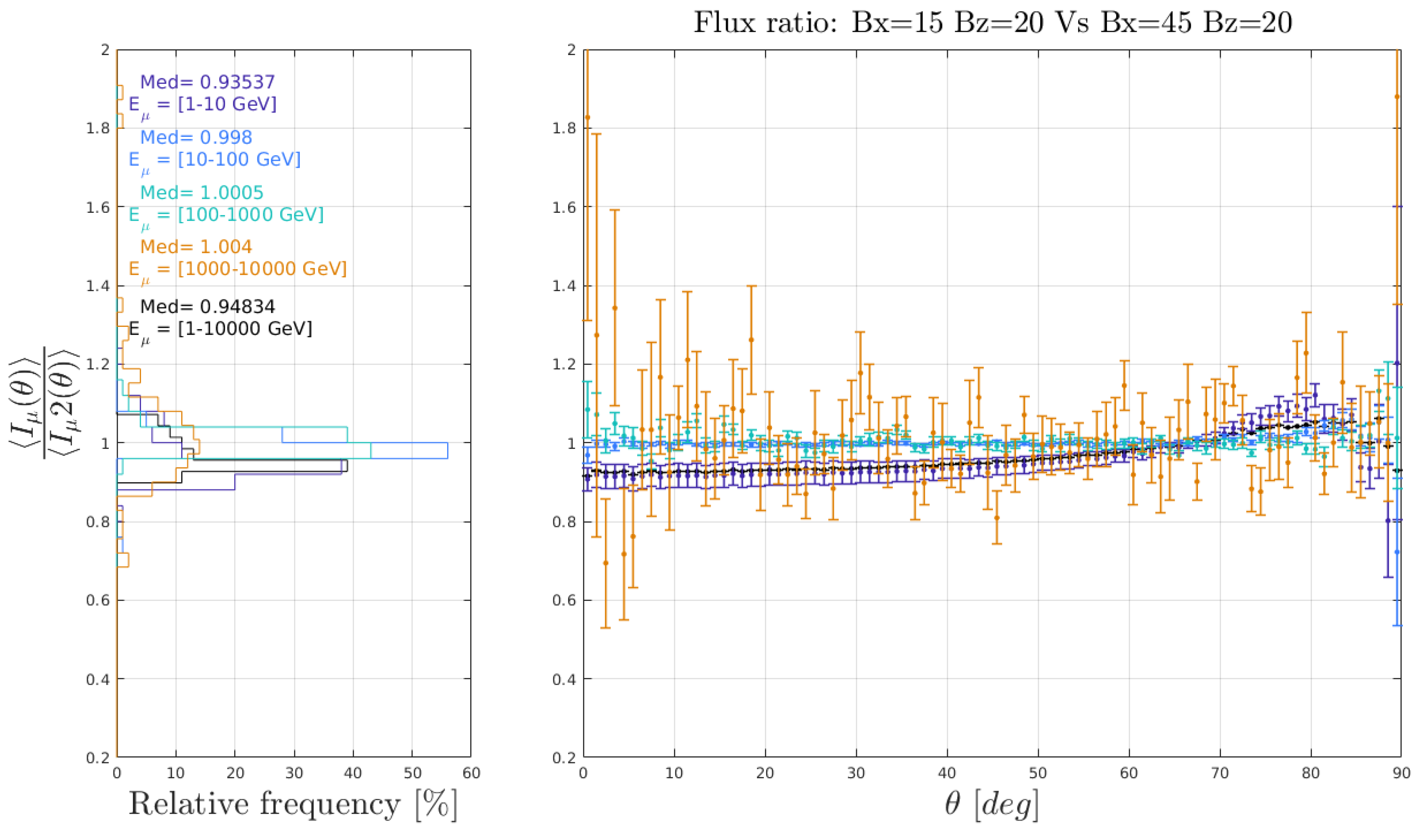
3.3.2. Geomagnetic Field Effects

In this part, the effects of the magnetic field are tested. For this purpose, the atmospheric and altitude parameters have been kept constant between the compared fluxes. We have set the vertical component as a constant ( B z = 20 µT) and the horizontal component ( B x = 15 µT) for a simulation of reference. We then compute another simulation by only changing B x = 45 µT. We simulated the muon flux with those two configurations and computed their ratio for four different energy ranges and different zenith angles.
Figure 9, on left panel, presents the normalized intensity distribution of the flux ratio over the zenith angle, for each individual energy range. The histogram of varying flux ratio values over zenith angle is meant to highlight the existence of systematic bias over the entire range of zenith values. It shows that when considering a higher energy range, the intensity ratios distribution (1– 10 4 GeV) tends to a narrow peak centered at 0.95 ± 0.01; the median value, corresponding to a small effect of about 5%. As expected the ratio tends to one for energy ranges greater than 10 GeV but affects the low-energy particles that are more deflected towards the poles. The right panel shows the flux ratio with respect to the zenith angle θ for fixed energy ranges. At low energies (1 to 10 GeV in dark blue) the flux is higher for B x = 45 µT until 60° and between 85° and 90°, and lower between 60 and 85°. This probably arises from the fact that high-angles particles have to cross a larger section of the atmosphere and therefore may start their travel with higher energies, making them less sensitive to the geomagnetic field’s effect. Note that this sample dominates over the total integrated flux ratio (in black), which follows more or less the same behavior. As expected, at high energies, typically above 10 GeV, the flux ratio remains more constant with the zenith angle (in light blue, green and orange). Note that this high energy sample is usually not used in scattering mode; therefore, one has to pick corrections for the geomagnetic effects to perform absolute measurement with scattering muography.
The same procedure is followed this time with a fixed horizontal component and various vertical components. We simulate the muon flux with these two configurations and we compute the ratio as a function of the energy and of the zenith angle. Only a slight difference at high zenith angles is observed. The B z component does not seem to affect the muon flux.

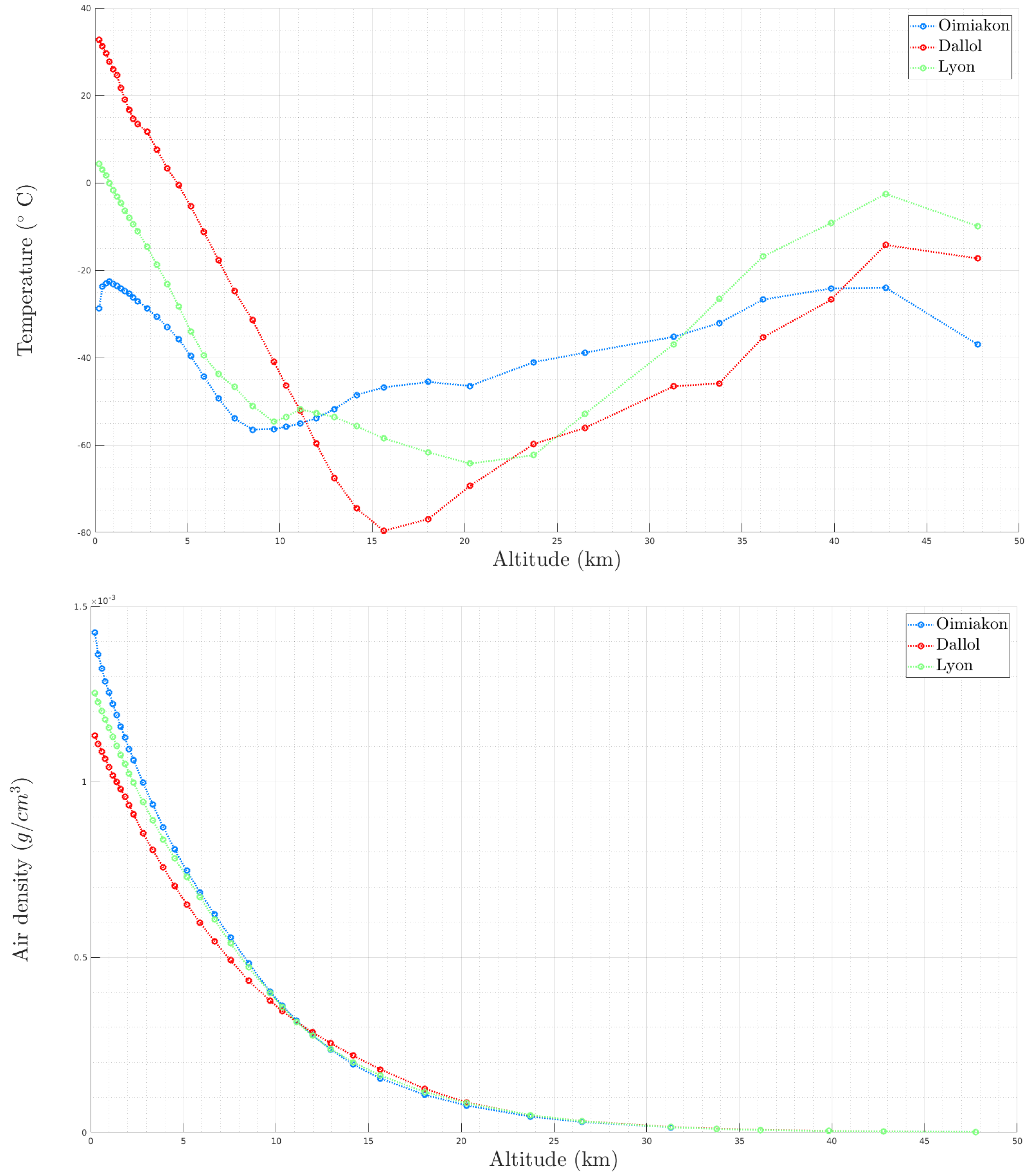
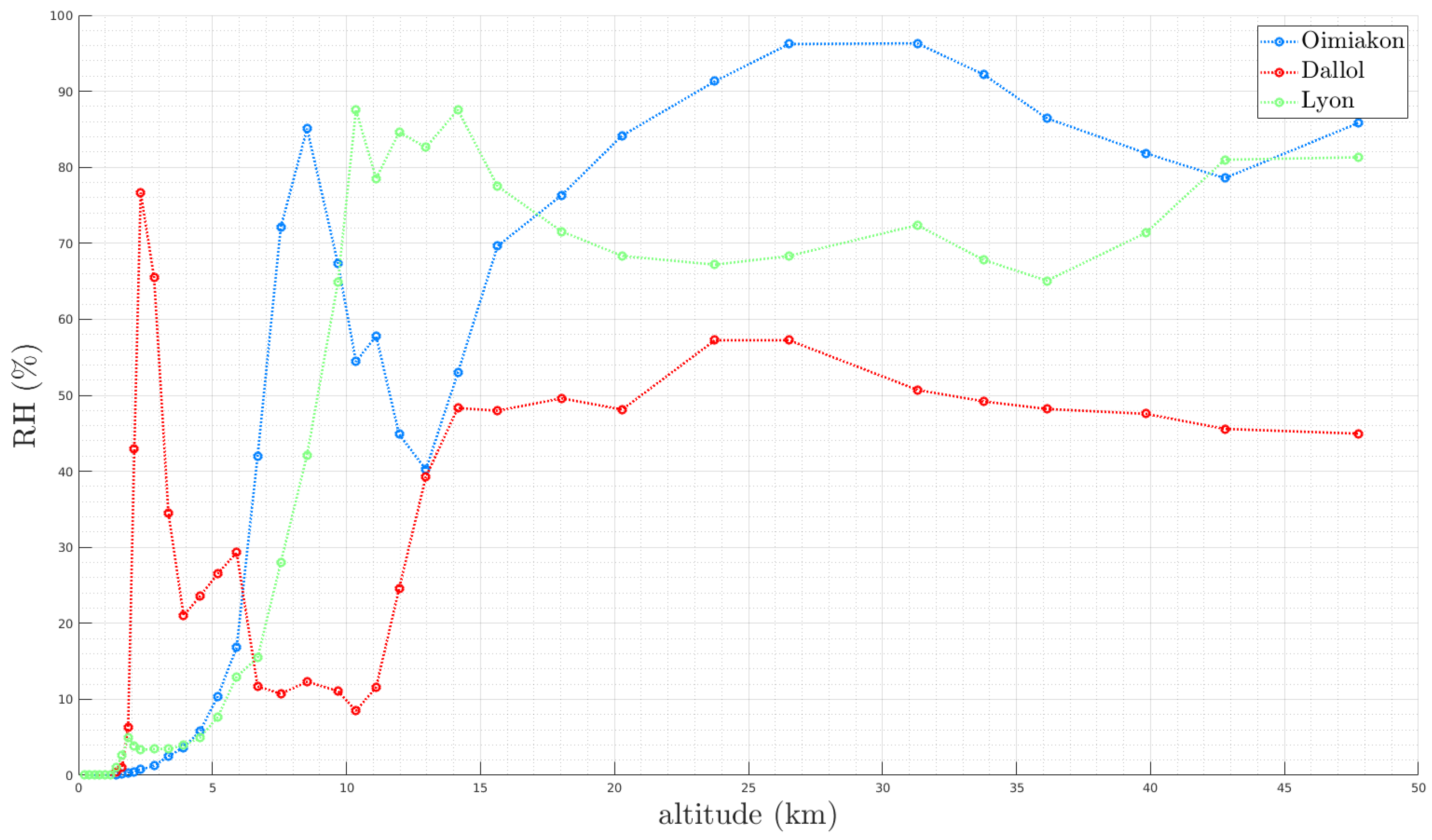
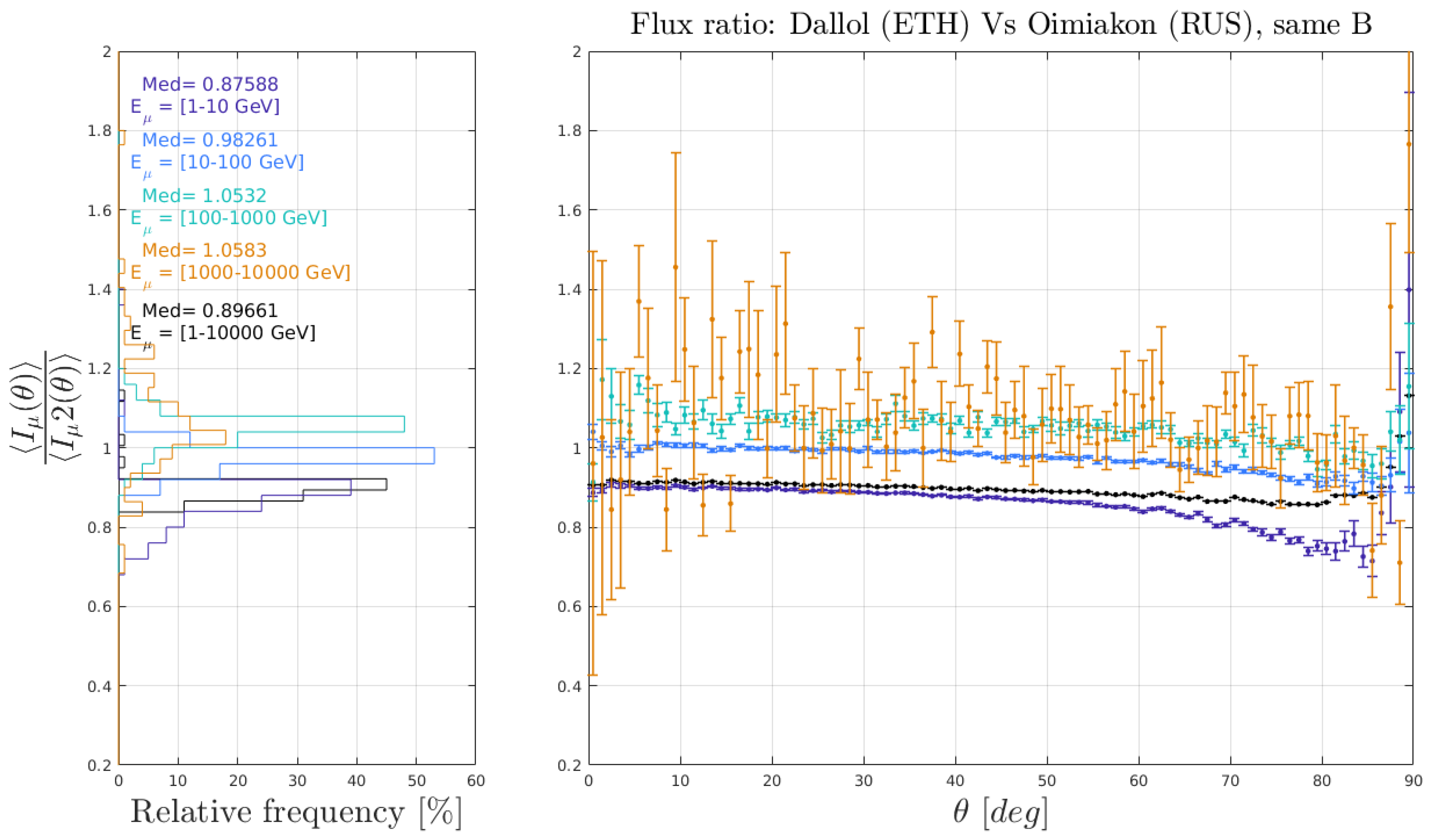
3.3.3. Atmospheric Thermodynamics Effects

We have tested the effects of altitude and magnetic field and their components on the muon flux. Finally we studied the impact of atmospheric density on the flux, which is ultimately controlled by the temperature and pressure state of the atmosphere. Hence, at the same location, seasonal variations affect the muon flux over time. For these tests we chose Dallol (Ethiopia) and Oimiakon (Russia) to test the effects of extreme temperature. These atmospheres are presented in the next subsection. The atmosphere density parameters used to simulate muon fluxes with CORSIKA are determined by using ERA5 datasets.
  • Atmosphere simple parametrization
Temperature and density profiles of Dallol, Oimiakon and Lyon are displayed in Figure 10. In Figure 11, relative humidity profiles are plotted for December 30th. We observe that the density of the atmosphere decreases with altitude, and that colder atmospheres are denser especially at lower altitudes. For the relative humidity profiles shown in Figure 11, the water vapor content in the air varies with altitude. Similar to temperature, relative humidity also depends on the pressure of the given system. It is low at ground level but important at high altitude. In very hot and/or dry atmospheres, it never reaches 100%.
  • Atmosphere properties
The atmosphere can be divided into five layers: the troposphere, stratosphere, mesosphere, thermosphere and ionosphere. The atmospheric profiles presented in Figure 10 stop at the end of the stratosphere (∼50 km). The troposphere is the part of the Earth’s atmosphere located between the surface and an altitude of about 8 to 15 km, depending on the latitude and the season. It is thicker at the equator than at the poles. This layer concentrates three quarters of the atmospheric mass and the temperature decreases rapidly with altitude. The stratosphere extends, on average, between 12 to 50 km. It is characterized by an increase in temperature with altitude. The stratosphere begins at low altitude near the poles, because the temperature is lower there. The distribution of atmospheric density is therefore different at opposite latitudes.
Despite the fact that the temperatures are very different at ground level, all temperatures decrease with increasing altitude (up to 10–15 km altitude) regardless of their location. Then, the temperatures increase in the stratosphere and decrease in the mesosphere. We notice that the change of behavior of the curve at Oimiakon is made at lower altitude. Indeed, the stratosphere starts lower at the pole. The relative humidity (RH) increases globally with altitude and is maximum at Oimiakon at high altitude, at 2 km Dallol have the highest RH and on the ground the values are almost the same everywhere on the globe in Figure 11.
Muons are typically produced at an altitude of 10–15 km (troposphere/stratosphere boundary). Their abundance is affected by the density differences in the atmosphere either by direct re-interaction or by modification of their parent mesons survival probabilities before decay [63,64]. The effect is more important for high-energy muons, which result from high-energy mesons with larger lifetime due to time dilation and therefore with longer paths in the atmosphere; thus, high-energy muons rates are more sensitive to temperature changes.
Figure 12 presents the normalized intensity distribution when considering different energy ranges: 1–10 GeV, 10–100 GeV, 100–10 3 GeV, 10 3 –10 4 GeV and the distribution for the whole energy range. The histogram of varying flux ratio values over zenith angle is meant to highlight the existence of systematic bias over the entire range of zenith values. It shows that when considering a larger energy range, the intensity distribution tends to a narrow peak centered at 0.90 ± 0.26, the median value, which means that the flux is 10% higher in Oimiakon (Russia) than in Dallol (Ethiopia); however, this statement is only valid for the integration over the total energy range. Right panel shows the flux ratio for different zenith angles θ in the range 0 to 90°, when considering the same energy ranges. It shows that in Dallol the flux is higher for high energies (100 to 10 4 GeV, in green and yellow), and lower in Oimiakon. For lower energies, the flux ratio is higher in Dallol (1 to 100 GeV, in light and dark blue), and lower in Oimiakon. These effects increase with the zenith angle θ . Statistical errors of fluxes simulations are fixed to 1 σ .
Knowing that Dallol is hotter than Oimiakon, we understand that the flux is higher in Oimiakon for high energy muons. At low energy, the integrated flux is higher in Dallol.
We estimated and summarized the maximum observed variations for the studied effects: magnetic field, altitude and state of the atmosphere (extreme and seasonal effect: summer vs. winter) for several muon energy ranges in Table 2. Altitude effect is the most impacting and the observed flux fluctuations are all dependent on the muon energy ranges for all effects. Seasonal effects have less impact than extreme atmospheres.

4. Conclusions

In this paper, we presented a muon flux simulation workflow accounting for muon-atmosphere interactions, based on the CORSIKA framework. We detailed our simulation strategy and the various relevant inputs from the hadronic interactions models to the atmosphere conditions. In particular, we used meteorological ERA5 pressure and temperature datasets to compute the required atmospheric density profiles. The workflow has been cross-validated against experimental evidences and standard semi-empiric models found in the literature. Simulations prove themselves to be a powerful tools to study and make predictions on tiny effects induced by the geomagnetic field, detection altitude or the atmospheric seasonal variations. The altitude effect seems to be the most important. In Lyon for example, at 1000 m altitude, the flux is 17% higher than at sea level. At medium latitude, seasonal effects affect the muon flux by modifying these proportions at high and low energy for a higher overall integrated flux at low temperatures (in winter). By analyzing the role of the temperature (and the atmospheric density) in this process with extreme atmospheres, we find the same results (∼10%). In contrast, the short term effects, such as an atmospheric depression, are not visible. An increase in the geomagnetic field exclusively increases the flux of low energy muons (∼5%) and only the horizontal component B x variation seems to play a role. Atmospheric impact appears to be dominant over the geomagnetic field effect for opposites latitudes (poles/equator). Those effects are of increasing importance when one wants to produce muon imagery and/or long-term internal state surveys, on both ends of the opacity spectrum. Low-opacity targets imagery is controlled by low-energy muons filtered out by the density of the atmosphere. On the other side, high opacity targets imagery is largely affected by the process at stake for high-energy muon production. This study opens the gate to develop semi-empiric formulas predicting the evolution of the muon energy spectrum for each zenith angle, in relation with the atmospheric state. These formulas will be useful to correct recorded muon fluxes on the fly, when direct open-sky measurements are not available or not sufficiently refined in terms of energy description.

Author Contributions

Conceptualization, A.C. (Amélie Cohu), J.M.; methodology, A.C. (Amélie Cohu), M.T.; software, A.C. (Amélie Cohu), M.T., A.C. (Antoine Chevalier); validation, J.M.; formal analysis, A.C. (Amélie Cohu); investigation, A.C. (Amélie Cohu); resources, J.-C.I., J.M.; data curation, J.M.; writing—original draft preparation, J.M.; writing—review and editing, J.M.; visualization, A.C. (Amélie Cohu); supervision, J.M.; project administration, J.M.; funding acquisition, J.M. All authors have read and agreed to the published version of the manuscript.

Funding

This research received no external funding.

Institutional Review Board Statement

Not applicable.

Informed Consent Statement

Not applicable.

Data Availability Statement

The ECMWF data are available from https://www.ecmwf.int/, accessed on 1 August 2022. Geomagnetic field components are generated by the NOAA geomagnetic calculator.

Acknowledgments

This work was the subject of a CIFRE agreement between the ArcelorMittal Maizières Research SA and IP2I (Lyon). We are grateful Justine Terrasse. We thank the editor and two anonymous reviewers for their constructive comments and suggestions, which helped to improve our work.

Conflicts of Interest

The authors declare no conflict of interest.

References

  1. Adamson, P.; Andreopoulos, C.; Arms, K.; Armstrong, R.; Auty, D.; Ayres, D.; Backhouse, C.; Barnett, J.; Barr, G.; Barrett, W.; et al. Observation of muon intensity variations by season with the MINOS far detector. Phys. Rev. D 2010, 81, 012001. [Google Scholar] [CrossRef] [Green Version]
  2. Tramontini, M.; Rosas-Carbajal, M.; Nussbaum, C.; Gibert, D.; Marteau, J. Middle-atmosphere dynamics observed with a portable muon detector. Earth Space Sci. 2019, 6, 1865–1876. [Google Scholar] [CrossRef] [Green Version]
  3. Jourde, K.; Gibert, D.; Marteau, J.; de Bremond d’Ars, J.; Gardien, S.; Girerd, C.; Ianigro, J.C. Monitoring temporal opacity fluctuations of large structures with muon radiography: A calibration experiment using a water tower. Sci. Rep. 2016, 6, 23054. [Google Scholar] [CrossRef] [PubMed] [Green Version]
  4. Tanaka, H.K.; Kusagaya, T.; Shinohara, H. Radiographic visualization of magma dynamics in an erupting volcano. Nat. Commun. 2014, 5, 3381. [Google Scholar] [CrossRef]
  5. Fehr, F.; The TOMUVOL Collaboration. Density imaging of volcanos with atmospheric muons. J. Phys. Conf. Ser. 2012, 375, 052019. [Google Scholar] [CrossRef] [Green Version]
  6. Lesparre, N.; Gibert, D.; Marteau, J.; Komorowski, J.C.; Nicollin, F.; Coutant, O. Density muon radiography of La Soufrière of Guadeloupe volcano: Comparison with geological, electrical resistivity and gravity data. Geophys. J. Int. 2012, 190, 1008–1019. [Google Scholar] [CrossRef]
  7. Jourde, K.; Gibert, D.; Marteau, J.; de Bremond d’Ars, J.; Komorowski, J.C. Muon dynamic radiography of density changes induced by hydrothermal activity at the La Soufrière of Guadeloupe volcano. Sci. Rep. 2016, 6, 33406. [Google Scholar] [CrossRef]
  8. Rosas-Carbajal, M.; Jourde, K.; Marteau, J.; Deroussi, S.; Komorowski, J.C.; Gibert, D. Three-dimensional density structure of La Soufrière de Guadeloupe lava dome from simultaneous muon radiographies and gravity data. Geophys. Res. Lett. 2017, 44, 6743–6751. [Google Scholar] [CrossRef] [Green Version]
  9. Morishima, K.; Kuno, M.; Nishio, A.; Kitagawa, N.; Manabe, Y.; Moto, M.; Takasaki, F.; Fujii, H.; Satoh, K.; Kodama, H.; et al. Discovery of a big void in Khufu’s Pyramid by observation of cosmic-ray muons. Nature 2017, 552, 386–390. [Google Scholar] [CrossRef] [Green Version]
  10. Procureur, S.; Attié, D. Development of high-definition muon telescopes and muography of the Great Pyramid. Comptes Rendus Phys. 2019, 20, 521–528. [Google Scholar] [CrossRef]
  11. Avgitas, T.; Elles, S.; Goy, C.; Karyotakis, Y.; Marteau, J. Mugraphy applied to archaelogy. arXiv 2022, arXiv:2203.00946. [Google Scholar]
  12. Alfaro, R.; Belmont-Moreno, E.; Cervantes, A.; Grabski, V.; López-Robles, J.; Manzanilla, L.; Martínez-Dávalos, A.; Moreno, M.; Menchaca-Rocha, A. A muon detector to be installed at the Pyramid of the Sun. Rev. Mex. Física 2003, 49, 54–59. [Google Scholar]
  13. Alvarez, L.W.; Anderson, J.A.; El Bedwei, F.; Burkhard, J.; Fakhry, A.; Girgis, A.; Goneid, A.; Hassan, F.; Iverson, D.; Lynch, G.; et al. Search for hidden chambers in the pyramids. Science 1970, 167, 832–839. [Google Scholar] [CrossRef] [PubMed] [Green Version]
  14. Guardincerri, E.; Rowe, C.; Schultz-Fellenz, E.; Roy, M.; George, N.; Morris, C.; Bacon, J.; Durham, M.; Morley, D.; Plaud-Ramos, K.; et al. 3D cosmic ray muon tomography from an underground tunnel. Pure Appl. Geophys. 2017, 174, 2133–2141. [Google Scholar] [CrossRef] [Green Version]
  15. Marteau, J.; de Bremond d’Ars, J.; Gibert, D.; Jourde, K.; Ianigro, J.C.; Carlus, B. DIAPHANE: Muon tomography applied to volcanoes, civil engineering, archaelogy. J. Instrum. 2017, 12, C02008. [Google Scholar] [CrossRef] [Green Version]
  16. Chevalier, A.; Rosas-Carbajal, M.; Gibert, D.; Cohu, A.; Carlus, B.; Ianigro, J.C.; Bouvier, F.; Marteau, J. Using mobile muography on board a Tunnel boring machine to detect man-made structures. In AGU Fall Meeting Abstracts; AGU: Washington, DC, USA, 2019; Volume 2019, p. NS43B-0839. [Google Scholar]
  17. Borozdin, K.; Greene, S.; Lukić, Z.; Milner, E.; Miyadera, H.; Morris, C.; Perry, J. Cosmic ray radiography of the damaged cores of the Fukushima reactors. Phys. Rev. Lett. 2012, 109, 152501. [Google Scholar] [CrossRef]
  18. Baccani, G.; Bonechi, L.; Borselli, D.; Ciaranfi, R.; Cimmino, L.; Ciulli, V.; D’Alessandro, R.; Fratticioli, C.; Melon, B.; Noli, P.; et al. The MIMA project. Design, construction and performances of a compact hodoscope for muon radiography applications in the context of archaeology and geophysical prospections. J. Instrum. 2018, 13, P11001. [Google Scholar] [CrossRef] [Green Version]
  19. Tang, A.; Horton-Smith, G.; Kudryavtsev, V.A.; Tonazzo, A. Muon simulations for Super-Kamiokande, KamLAND, and CHOOZ. Phys. Rev. D 2006, 74, 053007. [Google Scholar] [CrossRef] [Green Version]
  20. Shukla, P.; Sankrith, S. Energy and angular distributions of atmospheric muons at the Earth. Int. J. Mod. Phys. A 2018, 33, 1850175. [Google Scholar] [CrossRef]
  21. Honda, M.; Kajita, T.; Kasahara, K.; Midorikawa, S.; Sanuki, T. Calculation of atmospheric neutrino flux using the interaction model calibrated with atmospheric muon data. Phys. Rev. 2007, D75, 043006. [Google Scholar] [CrossRef] [Green Version]
  22. Guan, M.; Chu, M.C.; Cao, J.; Luk, K.B.; Yang, C. A parametrization of the cosmic-ray muon flux at sea-level. arXiv 2015, arXiv:1509.06176. [Google Scholar]
  23. Gaisser, T.K. Cosmic Rays and Particle Physics; Cambridge University Press: Cambridge, UK, 1990. [Google Scholar]
  24. Carminati, G.; Bazzotti, M.; Margiotta, A.; Spurio, M. Atmospheric MUons from PArametric formulas: A fast GEnerator for neutrino telescopes (MUPAGE). Comput. Phys. Commun. 2008, 179, 915–923. [Google Scholar] [CrossRef] [Green Version]
  25. Fedynitch, A.; Engel, R.; Gaisser, T.K.; Riehn, F.; Stanev, T. MCEq—Numerical code for inclusive lepton flux calculations. In Proceedings of the 34th International Cosmic Ray Conference PoS(ICRC2015), Hague, The Netherlands, 30 July–6 August 2015; p. 1129. [Google Scholar] [CrossRef] [Green Version]
  26. Fedynitch, A.; Becker Tjus, J.; Desiati, P. Influence of hadronic interaction models and the cosmic ray spectrum on the high energy atmospheric muon and neutrino flux. Phys. Rev. D 2012, 86, 114024. [Google Scholar] [CrossRef] [Green Version]
  27. Fedynitch, A.; Dembinski, H.; Engel, R.; Gaisser, T.K.; Riehn, F.; Stanev, T. A state-of-the-art calculation of atmospheric lepton fluxes. In Proceedings of the 35th International Cosmic Ray Conference (ICRC2017), Busan, Korea, 10–20 July 2017; p. 1019. [Google Scholar] [CrossRef] [Green Version]
  28. Fedynitch, A.; Riehn, F.; Engel, R.; Gaisser, T.K.; Stanev, T. Hadronic interaction model Sibyll 2.3 c and inclusive lepton fluxes. Phys. Rev. D 2019, 100, 103018. [Google Scholar] [CrossRef] [Green Version]
  29. Fedynitch, A.; Engel, R.; Gaisser, T.K.; Riehn, F.; Stanev, T. Calculation of conventional and prompt lepton fluxes at very high energy. arXiv 2015, arXiv:1503.00544. [Google Scholar] [CrossRef]
  30. Sato, T. Analytical model for estimating terrestrial cosmic ray fluxes nearly anytime and anywhere in the world: Extension of PARMA/EXPACS. PLoS ONE 2015, 10, e0144679. [Google Scholar] [CrossRef] [Green Version]
  31. Hagmann, C.; Lange, D.; Wright, D. Monte Carlo Simulation of Proton-Induced Cosimc Ray Cascades in the Atmosphere; Technical Report; Lawrence Livermore National Lab. (LLNL): Livermore, CA, USA, 2007. [Google Scholar]
  32. Hagmann, C.; Lange, D.; Verbeke, J.; Wright, D. Cosmic-Ray Shower Library (CRY); Lawrence Livermore National Laboratory Document UCRL-TM-229453; Lawrence Livermore National Laboratory: Livermore, CA, USA, 2012. [Google Scholar]
  33. Olàh, L.; Varga, D. Investigation of soft component in cosmic ray detection. Astropart. Phys. 2017, 93, 17–27. [Google Scholar] [CrossRef]
  34. Papini, P.; Grimani, C.; Stephens, S. An estimate of the secondary-proton spectrum at small atmospheric depths. Il Nuovo Cimento C 1996, 19, 367–387. [Google Scholar] [CrossRef]
  35. Agostinelli, S.; Allison, J.; Amako, K.a.; Apostolakis, J.; Araujo, H.; Arce, P.; Asai, M.; Axen, D.; Banerjee, S.; Barrand, G.; et al. GEANT4—A simulation toolkit. Nucl. Instrum. Methods Phys. Res. Sect. A Accel. Spectrom. Detect. Assoc. Equip. 2003, 506, 250–303. [Google Scholar] [CrossRef] [Green Version]
  36. Heck, D.; Schatz, G.; Knapp, J.; Thouw, T.; Capdevielle, J. CORSIKA: A Monte Carlo Code to Simulate Extensive Air Showers; Technical Report; Citeseer: State College, PA, USA, 1998; 6019. [Google Scholar]
  37. Heck, D.; Pierog, T. Extensive Air Shower Simulation with CORSIKA: A User’s Guide; Version 7.6300 from 22 September 2017; Institut für Kernphysik: Mainz, Germany, 2017. [Google Scholar]
  38. Clay, J. Penetrating radiation II. Proc. R. Acad. Sci. Amst. 1928, 31, 1091–1097. [Google Scholar]
  39. Biallass, P.; Hebbeker, T. Parametrization of the cosmic muon flux for the generator CMSCGEN. arXiv 2009, arXiv:0907.5514. [Google Scholar]
  40. Wentz, J.; Brancus, I.M.; Bercuci, A.; Heck, D.; Oehlschläger, J.; Rebel, H.; Vulpescu, B. Simulation of Atmospheric Muon and Neutrino Fluxes with CORSIKA. Phys. Rev. D 2003, 67, 073020. [Google Scholar] [CrossRef] [Green Version]
  41. Mitrica, B.; Brancus, I.; Rebel, H.; Wentz, J.; Bercuci, A.; Toma, G.; Aiftimiei, C.; Duma, M. Experimentally guided Monte Carlo calculations of the atmospheric muon and neutrino flux. Nucl. Phys. B-Proc. Suppl. 2006, 151, 295–298. [Google Scholar] [CrossRef]
  42. Pethuraj, S.; Majumder, G.; Datar, V.; Mondal, N.; Mondal, S.; Nagaraj, P.; Ravindran, K.; Saraf, M.; Satyanarayana, B.; Shinde, R.; et al. Azimuthal Dependence of Cosmic Muon Flux by 2 m × 2 m RPC Stack at IICHEP-Madurai and Comparison with CORSIKA and HONDA Flux. In Proceedings of the XXIII DAE High Energy Physics Symposium, Chennai, India, 10–15 December 2018; pp. 807–812. [Google Scholar]
  43. Kovylyaeva, A.; Dmitrieva, A.; Tolkacheva, N.; Yakovleva, E. Calculations of temperature and barometric effects for cosmic ray flux on the Earth surface using the CORSIKA code. Phys. Conf. Ser. 2013, 409, 012128. [Google Scholar] [CrossRef] [Green Version]
  44. Useche, J.; Avila, C. Estimation of cosmic-muon flux attenuation by Monserrate Hill in Bogota. arXiv 2018, arXiv:1810.04712. [Google Scholar]
  45. Hörandel, J.R. On the knee in the energy spectrum of cosmic rays. Astropart. Phys. 2003, 19, 193–220. [Google Scholar] [CrossRef] [Green Version]
  46. Wiebel-Sooth, B.; Biermann, P.L.; Meyer, H. Cosmic Rays VII. Individual element spectra: Prediction and data. arXiv 1997, arXiv:astro-ph/9709253. [Google Scholar]
  47. Spurio, M. The cosmic rays and our galaxy. In Particles and Astrophysics; Springer: Berlin/Heidelberg, Germany, 2015; pp. 23–54. [Google Scholar]
  48. Nesterenok, A. Numerical calculations of cosmic ray cascade in the Earth’s atmosphere -Results for nucleon spectra. Nucl. Instrum. Methods Phys. Res. Sect. B Beam Interact. Mater. Atoms 2013, 295, 99–106. [Google Scholar] [CrossRef]
  49. Pethuraj, S.; Datar, V.; Majumder, G.; Mondal, N.; Ravindran, K.; Satyanarayana, B. Measurement of azimuthal dependent cosmic muon flux by 2mx2m RPC stack near Equator at IICHEP-Madurai. arXiv 2019, arXiv:1905.00739. [Google Scholar]
  50. Heck, D. The CURVED Version of the Air Shower Simulation Program CORSIKA; Technical Report; Forschungszentrum Karlsruhe: Karlsruhe, Germany, 2004. [Google Scholar]
  51. Usoskin, I.G.; Kovaltsov, G.A. Cosmic ray induced ionization in the atmosphere: Full modeling and practical applications. J. Geophys. Res. 2006, 111, D21206. [Google Scholar] [CrossRef] [Green Version]
  52. Apel, W.; Asch, T.; Badea, A.; Bahren, L.; Bekk, K.; Bercuci, A.; Bertaina, M.; Biermann, P.; Blumer, J.; Bozdog, H.; et al. Progress in air shower radio measurements: Detection of distant events. Astropart. Phys. 2006, 26, 332–340. [Google Scholar] [CrossRef] [Green Version]
  53. Heck, D. Extensive Air Shower Simulations with CORSIKA and the Influence of High-Energy Hadronic Interaction Models. arXiv 2001, arXiv:astro-ph/0103073. [Google Scholar]
  54. Engel, R.; Heck, D.; Pierog, T. Extensive Air Showers and Hadronic Interactions at High Energy. Annu. Rev. Nucl. Part. Sci. 2011, 61, 467–489. [Google Scholar] [CrossRef]
  55. Tapia, A.; Dueñas, D.; Rodriguez, J.; Betancourt, J.; Caicedo, D. First Monte Carlo Simulation Study of Galeras Volcano Structure Using Muon Tomography. In Proceedings of the 38th International Conference on High Energy Physics, ICHEP 2016, Chicago, IL, USA, 3–10 August 2016. [Google Scholar]
  56. Atri, D. Hadronic interaction models and the angular distribution of cosmic ray muons. arXiv 2013, arXiv:1309.5874. [Google Scholar]
  57. Klepser, S. CORSIKA: Extensive Air Shower Simulation; Springer: Berlin, Germany, 2006; p. 29. [Google Scholar]
  58. Mitrica, B.; Petcu, M.; Saftoiu, A.; Brancus, I.; Sima, O.; Rebel, H.; Haungs, A.; Toma, G.; Duma, M. Investigation of cosmic ray muons with the WILLI detector compared with the predictions of theoretical models and with semi-analytical formulae. Nucl. Phys. B-Proc. Suppl. 2009, 196, 462–465. [Google Scholar] [CrossRef]
  59. Cazon, L.; Conceicao, R.; Pimenta, M.; Santos, E. A model for the transport of muons in extensive air showers. Astropart. Phys. 2012, 36, 211–223. [Google Scholar] [CrossRef] [Green Version]
  60. Velinov, P.; Mishev, A. Cosmic ray induced ionization in the atmosphere estimated with CORSIKA code simulations. C. R. Acad. Bulg. Des Sci. 2007, 60, 493. [Google Scholar]
  61. Abreu, P.; Aglietta, M.; Ahlers, M.; Ahn, E.; Albuquerque, I.F.d.M.; Allard, D.; Allekotte, I.; Allen, J.; Allison, P.; Almela, A.; et al. Description of atmospheric conditions at the Pierre Auger Observatory using the global data assimilation system (GDAS). Astropart. Phys. 2012, 35, 591–607. [Google Scholar] [CrossRef] [Green Version]
  62. Copernicus Climate Change Service Climate Data Store (CDS). ERA5: Fifth Generation of ECMWF Atmospheric Reanalyses of the Global Climate; CCCS: Singapore, 2017; Volume 15.
  63. Gaisser, T.K.; Engel, R.; Resconi, E. Cosmic Rays and Particle Physics; Cambridge University Press: Cambridge, UK, 2016. [Google Scholar]
  64. Grashorn, E.; De Jong, J.; Goodman, M.; Habig, A.; Marshak, M.L.; Mufson, S.; Osprey, S.; Schreiner, P. The atmospheric charged kaon/pion ratio using seasonal variation methods. Astropart. Phys. 2010, 33, 140–145. [Google Scholar] [CrossRef] [Green Version]
Figure 1. (Top) Primary cosmic ray fluxes (Hörandel [45], Papini [34] and Wiebel-Sooth [46]) for all components as a function of the energy of the primary particle. (Bottom) Ratio of these fluxes as a function of the energy of the primary particle.
Instruments 06 00024 g001
Figure 2. Slope coefficients of the primary spectra calculated with the [34,45,46] models as a function of the minimum value of energy range chosen in each simulation.
Instruments 06 00024 g002
Figure 3. CORSIKA’s coordinate system used [37].
Instruments 06 00024 g003
Figure 4. Different components of the magnetic field from NOAA. H is the magnetic north ( B x ) and Z the vertical component of the magnetic field.
Instruments 06 00024 g004
Figure 5. (Left panel) Histogram of flux ratio values computed over the zenith angle range (details are shown in the right figure) for several energy ranges from 10 to 10 4 GeV (in color) and for the whole energy range (in black). (Right panel) Flux ratio as a function of the zenith angle θ between (1) CORSIKA and (2) Tang et al. [19], for the same energy ranges as the left panel. The latter is the reference flux (ratio denominator). Med corresponds to the median value in each energy range.
Instruments 06 00024 g005
Figure 6. Differential relative muon fluxes (Flux/Mean Flux) simulated with CORSIKA and plotted as a function of the zenith angle and for several muon energy levels (different colors).
Instruments 06 00024 g006
Figure 7. Integrated muon fluxes I plotted as a function of the zenith angle θ . The crosses represent the measured data for different inclinations of the detector. The red line is a linear fit using c o s 2 ( θ ) on the total measured flux. The black line represents the simulated flux with CORSIKA.
Instruments 06 00024 g007
Figure 8. (Left panel) Histogram of flux ratio values computed over the zenith angle range (details are shown in the right figure) for several energy ranges from 1 to 10 4 GeV (in color) and for the whole energy range (in black). (Right panel) Flux ratio as function of the zenith angle θ in Lyon, France at (1) 1000 m of elevation and at (2) sea level, for the same energy ranges as the left panel. The second is the reference flux (ratio denominator). Same atmosphere and magnetic field for both fluxes were considered. Med corresponds to the median value in each energy range.
Instruments 06 00024 g008
Figure 9. Comparison of two simulations, with same atmosphere and altitude, and different magnetic fields. The magnetic parameters are (1) B x = 15 µT, B z = 20 µT and (2) B x = 45 µT, B z = 20 µT. The latter is the reference flux (denominator). (Left panel) Histogram of flux ratio values computed over the zenith angle range (details are shown in the right figure) for different energy ranges from 1 to 10 4 GeV (in color) and for the whole energy range (in black). (Right panel) Flux ratio dependence on the zenith angle θ between two different magnetic field fluxes for the same energy ranges as in the left panel. Med corresponds to the median value in each energy range.
Instruments 06 00024 g009
Figure 10. (Top) Temperature and (Bottom) density profiles for altitudes from 0 to 50 km of extreme atmospheres: Oimiakon (in blue) and Dallol (in red) and a moderate one, Lyon (in green).
Instruments 06 00024 g010
Figure 11. Relative humidity profiles for altitudes from 0 to 50 km of extreme atmospheres: Oimiakon (in blue) and Dallol (in red) and a moderate one, Lyon (in green).
Instruments 06 00024 g011
Figure 12. (Left panel) Histogram of flux ratio values computed over the zenith angle range (details are shown in the right figure) for several energies range from 1 to 10,000 GeV (in color) and for the whole energy range (in black). (Right panel) Flux ratio as a function of the zenith angle theta of two extreme temperature atmosphere for the same energy ranges as left panel. The different atmosphere conditions are (1) Dallol (Ethiopia) (2) Oimiakon (Russia), 12/30/20, with constant geomagnetic field and altitude. The latter is the reference flux (ratio denominator). Med corresponds to the median value in each energy range.
Instruments 06 00024 g012
Table 1. Energy thresholds values used by different authors and for this study.
E ThresholdHadronsMuonsElectronsPhotons
1. [57]0.1 GeV0.1 GeV0.1 MeV0.1 MeV
2. [58]0.2 GeV0.2 GeV0.1 MeV0.1 MeV
3. [59]0.05 GeV0.05 GeV0.003 GeV0.003 GeV
4. [52]300 MeV100 MeV250 keV250 keV
5. [60]0.05 GeV50 keV50 keV50 keV
6. This study0.05 GeV0.01 GeV0.001 GeV0.001 GeV
Table 2. Maximum observed variations comparing two CORSIKA fluxes for the studied effects: magnetic field, altitude and state of the atmosphere (extreme and seasonal effect) for several muon energy ranges.
1–10,000 GeV1–10 GeV1000–10,000 GeV
Magnetic field5 (±4)%6 (±1)%0.2 (±1)%
Altitude:
- 1000 m/0 m
- 5000 m/0 m

15 (±1)%
115 (±10)%

17 (±2.5)%
106 (±25)%

7 (±2.7)%
2 (±1)%
Atmosphere:
- Extreme
- Seasonal

10 (±7)%
8 (±1)%

13 (±10)%
9 (±3)%

5 (±10)%
2 (±10)%
Publisher’s Note: MDPI stays neutral with regard to jurisdictional claims in published maps and institutional affiliations.

