Article

Beyond the N-Limit of the Least Squares Resolution and the Lucky Model

by
Gregorio Landi
1,* and
Giovanni E. Landi
2
1
Dipartimento di Fisica e Astronomia, Universita’ di Firenze and INFN Largo E. Fermi 2 (Arcetri), 50125 Firenze, Italy
2
ArchonVR S.a.g.l., Via Cisieri 3, 6900 Lugano, Switzerland
*
Author to whom correspondence should be addressed.
Instruments 2022, 6(1), 10; https://doi.org/10.3390/instruments6010010
Submission received: 22 December 2021 / Revised: 12 January 2022 / Accepted: 26 January 2022 / Published: 29 January 2022

Abstract

:
A very simple Gaussian model is used to illustrate an interesting fitting result: a linear growth of the resolution with the number N of detecting layers. This rule is well beyond the well-known rule proportional to N for the resolution of the usual fits. The effect is obtained with the appropriate form of the variance for each hit (observation). The model reconstructs straight tracks with N parallel detecting layers, the track direction is the selected parameter to test the resolution. The results of the Gaussian model are compared with realistic simulations of silicon micro-strip detectors. These realistic simulations suggest an easy method to select the essential weights for the fit: the lucky model. Preliminary results of the lucky model show an excellent reproduction of the linear growth of the resolution, very similar to that given by realistic simulations. The maximum likelihood evaluations complete this exploration of the growth in resolution.

1. Introduction

Essential sources of information in high energy physics experiments are the tracking of ionizing particles. To accurately collect this information, large arrays of particle detectors (trackers) are installed in the experiments. Among the types of particle detectors, silicon micro-strip detectors are frequently selected as tracker components. A silicon micro-strip detector has a very special surface treatment (strips) able to give a set of localized signals (hit) to the readout system if an ionizing particle crosses the detector. The algorithms for track reconstruction are essential completions of the tracking systems and large efforts are dedicated to optimize their efficiency. Our refs. [1,2,3,4] were dedicated to these improvements and to demonstrate the essential importance of them to produce optimized linear fits. In refs. [1,2], we introduced for the first time very special probability density functions (PDFs), one for each hit, calculated for minimum ionizing particles (MIPs) crossing a micro-strip detector. Extensive expressions of those PDFs and the detailed derivations are reported in ref. [5] (and therein references) for illustration, ref. [6] reports the complete 3D plot of one of those PDFs. The PDFs are constructed around the properties of the hit positioning algorithms: the center of gravity (COG), the easiest and most frequently employed algorithm ( x g j = i = 1 j E i τ i / i = 1 j E i , where E i is the signal of the strip i, τ i its position and j the number of accounted strips). The COG is often indicated as a single algorithm, instead, it has different forms and properties depending by the number j of strip signals inserted in the algorithm. Each COG form has very different analytical and statistical properties. The mixture of different forms must be accurately avoided. In the present developments, the two or three strip COG (COG 2 or COG 3 ) are the only used forms. Due to their general expressions, containing ratios of random variables, Cauchy–Agnesi-like tails are present in their PDFs. The equations of ref. [2] evidence this property for the COG 2 algorithm. The long equations for the COG j PDFs of ref. [5] are only a part of our needs, to be useful in a fit, they must be completed with the functional dependence from the MIP impact point. This dependence is inserted with the functions of ref. [1], they were extracted from the data of a test beam with the use of a theorem demonstrated in ref. [1]. These functions are expressed with a Fourier series with many terms (150–200). The essential deviation of our complete probability distributions from Gaussian PDFs obliges the use of maximum likelihood method. With such complex functions, the maximum-likelihood method requires many cares to avoid the non-convergence of the search at the absolute maximum. To improve the convergence, we developed a lower level fitting tool (called schematic model) to be used as initialization of the likelihood exploration. The schematic model was built around effective variances extracted from the complete probability distributions, cutting their Cauchy–Agnesi-like tails to avoid divergences (ref. [2]). The η -algorithm gives the reconstructed hit positions [2] to use in the fits and is essential for the excellence of the results. The definition of effective variances (weight) for each hit allows the construction of the initial parameters for the likelihood exploration with a weighted least squares. The first application of our complete method was the reconstructions of straight tracks [1] for five detection layers. In this case, the likelihood is a surface and the convergence to the maximum can be easily verified. The results of the fits showed drastic improvements of the reconstructed track parameters compared to standard fits. The complete method is also able to obtain excellent fits in presence of large outliers; hence, this method eliminates the outliers from list of fitting problems. For its simplified form, the schematic model is unable to handle the outliers, but it is very realistic in all the other aspects. After acquiring confidence with straight tracks, we tested the reconstruction of tracks of MIPs in a homogeneous magnetic field [2]. In addition, the momentum reconstruction turns out much better than that of the standard fit. Reference [2] reports for the first time an interesting and unusual effect: an approximate linear growth of the momentum resolution with the number N of detecting layers. This result is strikingly different from the textbook result that easily demonstrates a growth in resolution as N in least-squares (or similarly for the Kalman filter). Although N refers to the fit of a constant, this type of rule will also be recalled for other fitted parameters where the rule is not so simple. The aim of this work is the illustration of the generality of the linear growth in resolution. For this, we study the fit of the track direction of a MIP crossing a simpler tracker at orthogonal incidence. The tracker model is formed by N detecting layers of identical technology, without magnetic field and exposed to a set of parallel tracks of high momentum MIPs (to neglect the multiple scattering). Our preferences for silicon micro-strip detecting layers is due to our availability of effective simulations; however, this condition is not essential as we will show. The simplicity of some simulations gives a direct explanation of the results of our complete fitting method. Let us briefly recall the principal assumptions contained in the standard least-squares method. Almost always, identical variance for all measurements is assumed [7,8]. For example, ref. [8] cites this condition in each of its chapters. The identity of the variances is defined in statistics as homoscedasticity. It introduces a drastic shortcut in the least squares equations that become independent from the data variances and the origin of the data, thus extensible to any type of fitting problem. The opposite of homoscedasticity is indicated as heteroscedasticity. In this case, the identity of the variances is abandoned. The equations for the least-squares report the weighted form (as in ref. [9]); however, without additional mathematical tools (as those we developed for this type of problems) it is impossible to consistently handle the forms of heteroscedasticity. In any case, the complexity introduced by heteroscedasticity destroys the independence from the origin of the data, but adds substantial improvements to the fit quality. To illustrate this point, beyond the results of refs. [1,2] and their long maximum likelihood searches, a simple Gaussian model will be tested. The model also easily shows the generation of the linear growth with N of the resolution with a very simple form of heteroscedasticity (minimal heteroscedasticity). This Gaussian model is compared with a more realistic model (the schematic model of refs. [1,2]). We limit the schematic model to a single detector type, very similar to silicon strip detectors largely used in running CERN-LHC experiments [10,11,12]. A preliminary introduction of a fast suboptimal tool (the lucky model) will be discussed and compared with the schematic model. We restrict our discussion to the recipes to obtain these results. Mathematical details are published in dedicated papers [3,4,5] and therein references with further examples inspired to the following Gaussian model and of some easy extensions, the two other discussed in ref. [13]. References [3,4] demonstrate the essentiality of our approach to get a statistical optimality of the least-squares fits. To complete these fitting results a comparison with the maximum likelihood evaluations (or maximum probability in ref. [13]) is reported at the end. All these results underline new possibilities of producing important improvements in data analysis of tracker signals. The excellent quality of the detectors inserted in the trackers and their continuous evolving technology requires all the possible analytical efforts to extract the best from them. The usual fitting methods are a crude simplification of the methods discussed in ref. [13], tuned on the problems of that times, completely out of place with our very sophisticated silicon detectors.

2. A Simple Gaussian Model and the Linear Growth

The explored application is a Gaussian model with two different standard deviations ( σ ), one of 0.18 (in unity of the strip width 63 μ m) with a probability of 80% and the other of 0.018 with a probability of 20%: hard symmetry with a small “spontaneous” symmetry breaking (minimal heteroscedasticity). The relation of this model with the schematic model of silicon micro-strips is illustrated in Figure 1, and represents a drastic simplification of the models of refs. [1,2]. Experimental hints of the border effect, evident in Figure 1 as a strong decrease of the effective σ , are reported in ref. [14] for gas ionization chambers.
Few lines of MATLAB [15] code suffice to produce this simulation, and they could be a viable substitute of long mathematical developments. A large number of Gaussian random numbers, with zero average and unity standard deviation, are generated (with the MATLAB randn function). Each one is multiplied by one of the two standard deviations ( 0.18 , 0.018 ) with the given relative probability ( 80 % , 20 % ). The data are scrambled and recollected to simulate a set of parallel tracks crossing few detector layers. This data collection simulates a set of tracks populating a large portion of the tracker system with slightly non-parallel strips on different layers (as it always is in real detectors). The detector layers are supposed parallel, but for the non-parallelism of the strips, the hit positions of a track, relative to the strip centers, seem to be uncorrelated. The properties of the binomial distribution produce the linear growth. Due to the translation invariance, the tracks can be expressed by a single equation x i = β + γ y i with β = 0 and γ = 0 for the orthogonal incidence of the set of tracks ( β is the impact point of the track, γ the direction, y i the positions of the detector layers and x i the hit position). The distributions of γ f , the γ value given by the fit, are the object of our study. The γ distribution is a Dirac δ -function, as it is usual to test the resolution of the fitted values γ f . The distance of first and the last detector layer is the length of the PAMELA [16] tracker (445 mm , 7063.5 in strip width, for different lengths γ f scales as usual in least-squares). Other “detector layers” are inserted symmetrically in this length. Two different least squares fits are compared. One suppose identical σ of each hit and utilizes the usual equations for homoscedastic systems (we call this standard fit). The other fit applies the appropriate σ -values to each hit. This second fit shows a linear growth in the resolution (as far as a set of random variables can follow this rule). We generate 150,000 tracks for each configuration.
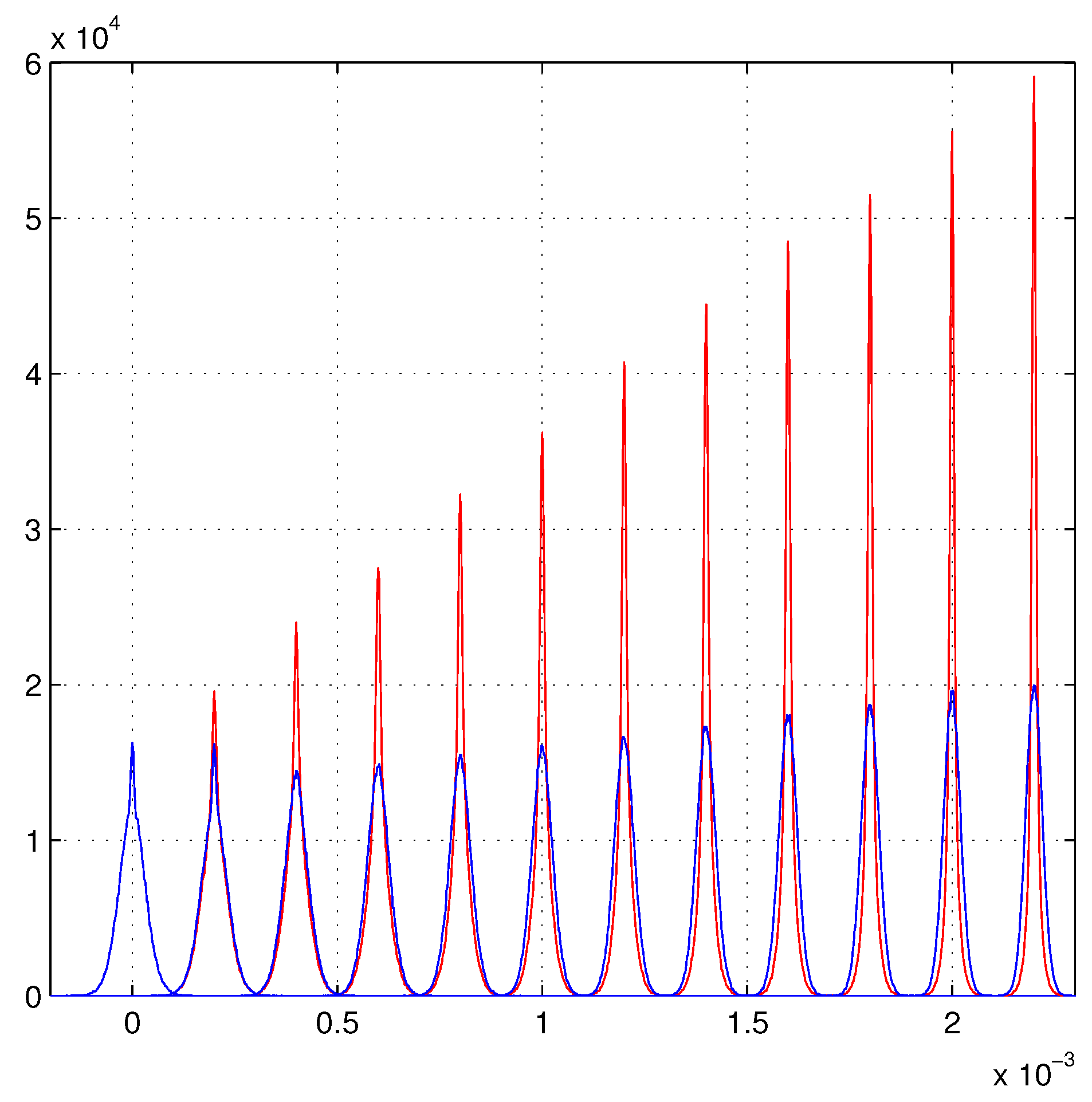
The results are reported in Figure 2 as (empirical) probability density functions of γ f . The parameter γ f is the tangent of a small angle, a pure small number. To give a scale to the plots of γ f , we could identify the tangent with its argument and consider the horizontal scale in radians (rad) and the vertical scale as rad 1 . We will neglect all these details in the plots that report probability density functions of pure number variables. All the distributions we have to plot are centered around their fiducial value γ = 0 for each number N of layers. For clarity of the plot, the distributions with two layers is centered on zero. The others with three, four, etc., up to thirteen layers are shifted by N 2 identical steps to show better their increase. (This rule is extended to all similar plots.) Heteroscedasticity also influences the first two distributions (two and three layers) in the standard fit. In fact, if the two hits of a track have a narrow (Gaussian) position distributions (small σ ), the γ f of the fitted tracks is forced to be contained in a narrow distribution. It is curious that to reach the height of these two distributions the standard fits require many additional layers. We will consider the height of each distribution as an evaluation of the resolution of the corresponding fit. In fact, the most common distributions have the maximum proportional to the inverse of the full-width-at-half-maximum (FWHM). The FWHM is often considered a measure of the mean error for non-Gaussian distributions and its inverse is the resolution. If the detector layers are slightly different (as usual) the linear growth will show small distortions due to these differences.
An approximate linear growth can also be extracted from the standard least squares, as illustrated in Figure 3.
In fact, for a pure homoscedastic Gaussian model, it is a basic demonstration [7] that the fitted parameters are independent random variables (easily verified in these simulations using a single average σ ). The presence of a small heteroscedasticity destroys this independence and tends to couple the probability distribution of γ f with the values of ψ 2 = i ( x i β f γ f y i ) 2 for each track. The parameters β f and γ f are those given by the fit of that track. Among the lowest values of the ψ 2 , good γ f -values are more frequently found. The Gaussian model shows a partial linear increase of the γ f distributions selected with ψ 2 . The empirical equation ψ 2 < 0.08 ( N / 13 ) 2 is used to accumulate a sufficient number of ψ 2 -values to produce clear γ f -distributions. Figure 3 shows the resulting distributions, this correlation is an independent test of heteroscedasticity.

3. The Schematic Model

Similar results can be obtained from our schematic model. This realistic model is called schematic in refs. [1,2]. In those works, the schematic model was used as first approximation of the complete model and as starting point for the maximum likelihood search. The quality of the fit produced by the schematic model is not far from the complete model, the main differences are in the ability of the complete model to also find good results in the presence of the worst hits (outliers). The calculations of the effective variance of each hit is very time consuming, but after an initial (large) set of σ is obtained, the others can be quickly produced with interpolations (high precisions are inessential). We always used the time consuming procedure. Figure 1 shows a subset of effective σ for this type of micro-strip detectors. An interesting aspect of this scatter-plot is the very low values of σ at the strip borders. The positioning algorithm is the η -algorithm of ref. [17], briefly summarized in ref. [2]. This algorithm is essential to eliminate the large systematic errors of the two strip center of gravity (COG 2 ). The forms of those systematic errors were analytically described in ref. [18], many years later than their full corrections. References [19,20] added further refinements to the η -algorithm and extended it to any type of center-of-gravity (COG) algorithm.
We underline that the results, shown in the following, are impossible without the η -algorithm. For example, the COG 2 algorithm degrades its (modest) results with this refined approach. It is uncertain that the statistics has any relation with least squares fits based on COG positioning algorithms. We proved in ref. [2] that the elimination of any random noise (the statistics) does not modify the probability distributions of the fitted parameters based on the COG 2 positions. Instead, the distributions of the fitted parameters based on the η -algorithm rapidly converge toward Dirac- δ functions, as expected.
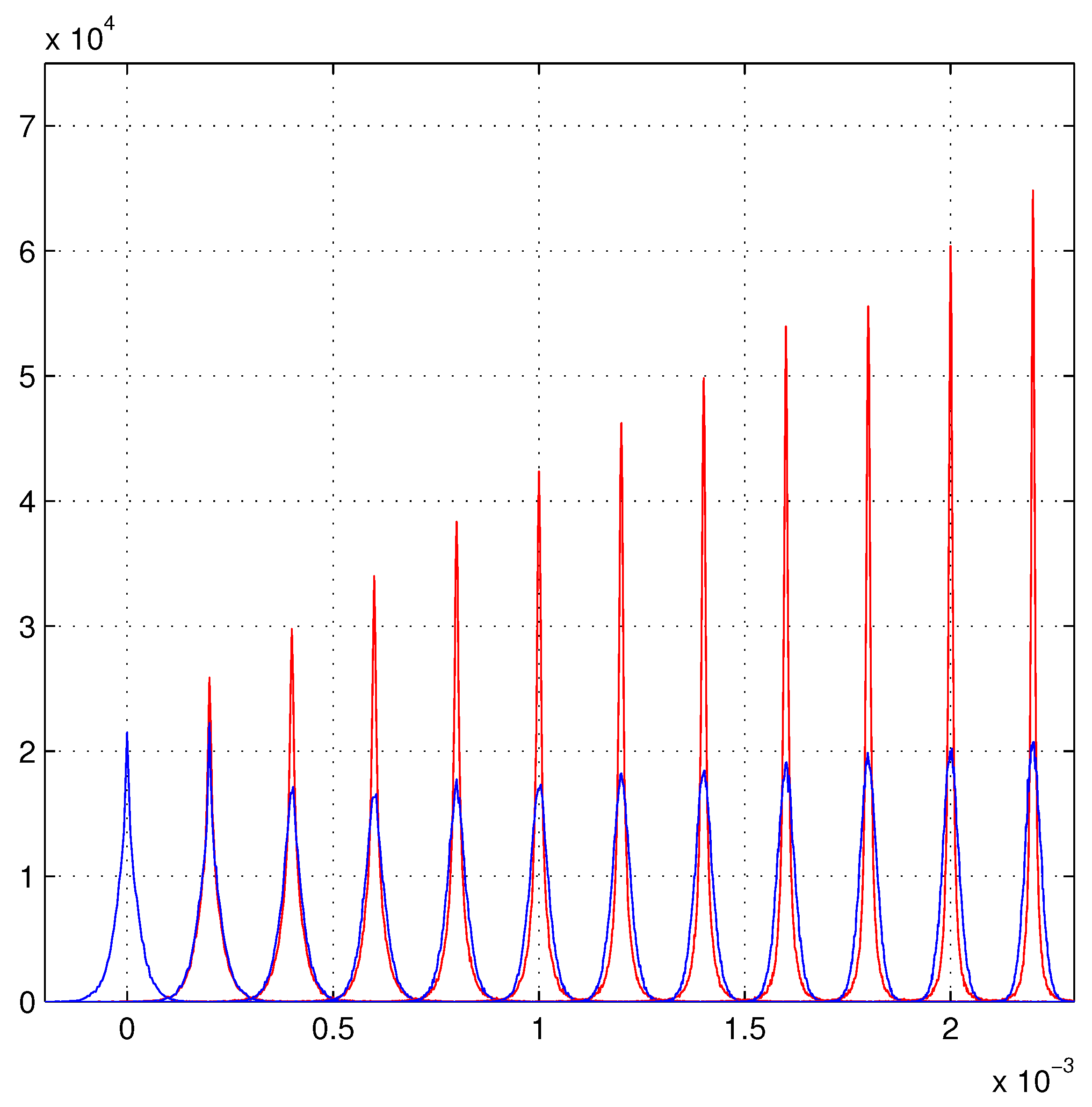
Again, our aim will be the fit of straight tracks of equation x i = β + γ y i with β = 0 and γ = 0 incident orthogonally to a set of detector layers. The properties of the simulated hits are modeled as near as possible on test-beam data [16], as discussed in ref. [1]. Again, we compare the γ f distributions given by two types of least squares. One fit uses the different σ (the blue dots) of the scatter plot of Figure 1 for the hits, and the standard least squares that assumes an identical variance for each hit. Figure 4 shows these results.

4. The Lucky Model

In Figure 1 of ref. [2], a large asymmetry is evident in one of the two scatter plots. Given our selection of an orthogonal incidence, symmetry is expected, but our long list of equations, required to arrive to the effective variances, produce this asymmetry. The sole tentative explanation was the strong similarity of our scatter plots with the COG 2 histograms of the original data. One of the two histograms has the corresponding asymmetry [1]. The data were collected in the test beam of ref. [16]. Our preliminary analysis did not find any simple relation (scaling factors) able to reproduce the plots. The cut selection, we used in the definition of the effective variances (ref. [2]), were essentially based on an aesthetical criterion. We considered relevant the reproduction of parts of the Gaussian features when they were present. Essentially, we tuned the cuts on a small subset of excellent hits to seek a comparison with our complete probability distributions. The scatter plots of ref. [1] were produced for the first time just for their insertion in the publication. However, once we discarded the possibility of a casual matching, a reasonable explanation could be found of this coincidence. Thus, a more accurate analysis was undertaken. The use of the equations of ref. [2] allows the construction a very approximate demonstration of the consistency of the trends of our scatter plots. A by-product of that analysis is a geometrical support to the resolution increase at the strip borders, just the origin of the linear growth. All the details of this preliminary demonstration will be published elsewhere. Figure 5 illustrates the very rough matching of the σ scatter plot and the COG 2 histogram. The σ -values are scaled to produce an approximate overlap with the COG 2 histogram. More precisely, we plot the normalized histogram divided by the bin size and interpolated with a Fourier series, the red line is a merged set of dots produced by the interpolation. One red dot for each blue dot.
For completeness, we recall the intuitive explanation given in ref. [1] about this similarity. The effective σ estimates the ranges of the possible impact values converging to the same COG 2 value. Hence, larger σ gives higher COG 2 probability and lower σ gives lower COG 2 probability. Inverting this statement, it looks reasonable to suppose that hits with the lower COG 2 probability have lower effective σ and hits in the higher COG 2 probability have higher effective σ . If these assumptions would be successful we have a very economic strategy to implement heteroscedasticity in the track fitting with pieces of information that were well hidden: just in front of us. However, without the hints of the scatter plots of ref. [1], they could remain hidden. The COG 2 probabilities are very easy to obtain from the corresponding histograms or as a by-product of the η -algorithm [19]. Further details are required: the scaling factors to render compatible the COG 2 histograms and effective σ scatter plots. In general, these scaling factors must be calculated. However, for identical detectors, as in this case, an identical factor is required and it becomes irrelevant for the linearity of the (weighted) least squares equations. Hence, we can attempt to directly use the amplitude of histogram as rough effective σ and observe the effects in the fit.

The Linear Growth in the Lucky Model

The “lucky” results are illustrated in Figure 6 for this “lucky” model. This figure is produced as Figure 4 with the sole difference given by the use of the rough effective σ in the weighted least squares.
The maximum of Figure 6 is around 6.5 × 10 4 and Figure 4 is around 7.2 × 10 4 (a difference of 10 % ): the results of the fits are excellent. The robustness of the heteroscedasticity is evident. Large variations of the details of the parameters (probability distributions) of the models do not modify the fit results. For example, the use of the effective variances, illustrated with the red line in Figure 1, with the η -positioning gives γ f -distributions very similar to the complete schematic model. This result is easy to justify, the weights inserted in the least squares are σ 2 , and the higher σ -values are all compressed near to zero, and their differences, compared to the constant value of Figure 1, become negligible. Instead, the lower σ -values are very similar in the two models and they dominate the fits, exactly as for the lucky model. Another connection is contained in the lucky model; the functional form of σ 1 as a function of η is a well-known function introduced with a theorem in ref. [18] and illustrated in ref. [19]. This function is the average shape of the MIP signal collected by the strip; hence, higher signal density gives better hits.
We also test the lucky model approximation with the three strip COG (COG 3 ) histogram and its corresponding η positioning ( η 3 ). Furthermore, here, the linear growth is clearly evident but the maximum is around 1 / 2 of that of Figure 4. The strip added to the COG 2 , to compose the COG 3 , is almost always pure noise at this orthogonal incidence [19]. In addition, the COG 3 has discontinuities at the strip borders [18], here very small and masked by the noise, but just in the region with the best σ . Thus this lower result is not unexpected, and it is consistent with our full three strips schematic model. Similar tests were also performed on the low noise floating strip side of ref. [1].

5. Hints for an Experimental Verification

Part of the results presented here could be verified with a test beam. The beam divergence should be less than 10 5 radians, probably not easy to obtain [21]. In the simulations we used a very simplified (for the computer) approach: the detector-layer configurations were generated each time dividing symmetrically the allowed interval from the first and last layer. This corresponds to a different experimental set-up for any layer number. A more realistic set-up could be composed with a fixed number of parallel detector layers, (normal silicon micro-strips) orthogonal to the beam (of high momentum to limit the multiple scattering). An effective increase of the layer number can be produced varying those inserted in the fit. Excellent precision in the tracker alignment parameters and a very small beam divergence are required for a direct test of the linear growth. The η -algorithm is always essential. At orthogonal incidence and without magnetic field, the corrections of the η -algorithm of refs. [19,20] are very small or negligible. In any case, for parallel tracks, the corrections are identical and their neglect implies a parallel translation of the tracks. The ψ 2 and the lucky model can be used to test heteroscedasticity.
If the beam divergence is large compared to the γ f -resolution of the fit, the presence of the linear growth in resolution can be observed in the fluctuation of the difference of the γ f fitted with all the available layers and the γ f fitted with the elimination of a layer each time in the same track. The linear growth produces a parabolic increase of these differences. Instead, the standard fit produces a small increase in the last couple of differences.

6. Linear Growth of the Maximum Likelihood Evaluations

The main part of the previous discussion is concentrated on the least-squares method and on the essential differences of the consistent fits of heteroscedastic systems from the fits with homoscedastic equations. We have to recall that only for Gaussian PDFs the least-squares method is the top level of fitting, in the sense that the least-squares method coincides with the maximum likelihood evaluation. For other PDFs, the maximum likelihood is able to improve the fit beyond the least-squares results. Thus, given our principal aims toward the maximization of fit quality, the maximum likelihood evaluations for the fits of Figure 4 is an essential completions. The following figures are devoted to these comparisons. The schematic model is used as starting point for the numerical search of the maximums of the products of PDFs as that of ref. [6]. The linear growth of the schematic model is reinforced by these additional developments. To save the consistency with the previous figures, we changed slightly our convention of refs. [1,2]: the black lines are the maximum likelihood evaluations. The schematic model results are the red lines that partially cover the black lines. The improvements beyond our best least-squares is substantial, the maxima of the γ f empirical PDFs are clearly higher and rate of the linear growth is faster.
Following the standard books on mathematical statistics and the suggestion of Gauss [13] we also show a comparison among the variances (or the standard deviations) of the empirical PDFs for the γ f of Figure 7, in any case remembering the complications of the realistic PDFs [2,5] with their Cauchy–Agnesi tails and the possible meaningless of mean square calculations of random variables (mathematical divergences and other well known anomalies on finite set of data). However, as discussed in ref. [4], we abandon the use of the variance as tool to estimate the fit quality in favor of the maxima of the distributions (for almost triangular distributions, as ours, the inverse of the maximum is the full width at half maximum). In any case, the variance is also of rare use in tracker physics for the clear evidences of non-Gaussian tails. The preferred method is the fitting of a Gaussian PDF in the core of the distribution (as in refs. [12,14]). This way circumvents the effects of the heavy tails of the PDFs in the variance calculations. Reference [4] analytically shows the large increase in the numerical values of the resolution given by the application of this method to narrow distributions.
As in ref. [4] we did not report in Figure 8 the variances or the standard deviations, instead we make comparisons using the parameter H G = 1 / ( 2 π Σ D ) were Σ D is the variance ( Σ D the standard deviation), H G is the maximum of a Gaussian PDF with Σ D as standard deviation. This parameter amplifies the differences among different fits allowing better comparisons. Straight lines are inserted in Figure 8 to guide the eyes. As easily observed, the differences from Gaussian PDFs are very clear, the standard least-squares PDFs for N > 4 are the most similar to Gaussian PDFs, the maxima are slightly higher then the corresponding H G , these small differences are evidently due to the Cauchy–Agnesi tails of the realistic PDFs. Instead, the PDFs of the Gaussian toy-model are almost coincident [4] for N > 4 . For the schematic model and the maximum likelihood evaluations, the parameters H G are much higher than those of the standard least squares, but substantially lower than the maxima of the empirical PDFs.
The rapid growth of the parameters H G for the maximum likelihood evaluations compared to those of the schematic model indicated a beneficial effect on the tails of the γ f -PDFs, as expected.
The growth of the H G -parameters of the standard least-squares is very close to that of the homoscedastic systems ( a part the random fluctuations of the variance) that has complicated dependence from N: N ( N + 1 ) / ( N 1 ) . This rule becomes similar to the N of the impact point ( β f ) for not too small N. For this range of N-values the trend of H G looks almost linear.
We never discussed the distributions of the impact parameter β f for the difficulties to invent systems to measure the resolution. In any case, the distributions of β f show a linear growth for the schematic model and for the maximum likelihood evaluations with relative amplitudes compatibles with those of γ f . The standard least-squares has a weak growth as N for not too low N.

Beyond the Present Maximum Likelihood Evaluations

The maximum likelihood evaluations show the top level in γ f resolution. This approach requires very complex procedures and mathematical tools, we developed the required tools but with different level of refinements. Thus, a careful analysis of those steps could add further improvements to these results. We published almost all the essential elements of this procedure. One of first tool requiring improvements could be the routine to search the likelihood maximum (or better the minimum of its negative logarithm), we used a standard MATLAB function fminsearch that is optimized for very general problems, in this case, it could be too slow in the minimum search.

7. Conclusions

Simple simulations produce linear growths in the fit resolution with the number N of detector layers, similar to those of ref. [2] for the momentum reconstruction. Sets of parallel straight tracks are simulated for the fits, and the test parameter is the direction γ of the tracks. The two-parameter fit is easier than that for the momentum. The Gaussian model easily produces the linear growth of the resolution for the fitted parameters. The model is so simple, for its essential mathematics, that it can be completed with few lines of MATLAB code and its results are very similar to our very complicated schematic model. The evident similarity of the effective σ scatter-plots with the histograms of the two strips center of gravity triggered a more accurate analysis of its origin. This analysis was sufficiently convincing to try a weighted least squares fit with weights directly extracted from the center of gravity histogram (the lucky model). The result of this test is excellent with a drastic increase of the fit resolution and the sought linear growth. The differences of the lucky model, compared to the schematic model, are around 10 % , a negligible price compared to the enormous simplification in the the extraction of the weights. Evidently, that these are preliminary results, further tests are essential before a systematic use of the model. Very synthetic indications are given for an experimental verification of the model. A final comparison with the maximum likelihood evaluations is reported, the non Gaussian expressions of the realistic probability distributions also allow this further increase in resolution well beyond that of the schematic model.

Author Contributions

Conceptualization, G.L. and G.E.L.; methodology, G.L. and G.E.L.; software G.L. and G.E.L. All authors have read and agreed to the published version of the manuscript.

Funding

This research received no external funding.

Conflicts of Interest

The authors declare no conflict of interest.

Abbreviations

The following abbreviations are used in this manuscript:
PDFprobability density function
MIPminimum ionizing particle
COGcenter of gravity
COG n center of gravity algorithm with n-strips

References

  1. Landi, G.; Landi, G.E. Improvement of track reconstruction with well tuned probability distributions. J. Instrum. 2014, 9, P10006. [Google Scholar] [CrossRef] [Green Version]
  2. Landi, G.; Landi, G.E. Optimizing momentum resolution with a new fitting method for silicon-strip detectors. Instruments 2018, 2, 22. [Google Scholar] [CrossRef] [Green Version]
  3. Landi, G.; Landi, G.E. The Cramer-Rao inequality to improve of the resolution of the least-squares method in track fitting. Instruments 2020, 4, 2. [Google Scholar] [CrossRef] [Green Version]
  4. Landi, G.; Landi, G.E. Generalized inequelities to optimizing the fitting method for track reconstructions. Physics 2020, 2, 35. [Google Scholar] [CrossRef]
  5. Landi, G.; Landi, G.E. Probability Distributions of Positioning Errors for Some Forms of Center-of-Gravity Algorithms. Part II. arXiv 2020, arXiv:2011.14474. [Google Scholar]
  6. Landi, G.; Landi, G.E. Silicon Micro-strip Detectors. Encyclopedia 2021, 1, 82. [Google Scholar] [CrossRef]
  7. Ivchenko, G.; Medvedev, Y. Mathematical Statistics; Mir Publishers: Moscow, Russia, 1990. [Google Scholar]
  8. Devore, J.L.; Berk, K.N. Modern Mathematical Statistics with Applications; Springer: New York, NY, USA, 2018. [Google Scholar]
  9. Olive, K.A.; Agashe, K.; Amsler, C.; Antonelli, M.; Arguin, J.-F.; Asner, D.M.; Baer, H.; Band, H.R.; Barnett, R.M.; Basaglia, T.; et al. Particle Data Group. Chin. Phys. C 2014, 38, 090001. [Google Scholar] [CrossRef]
  10. ALICE Collaboration. The ALICE experiment at the CERN Large Hadron Collider. J. Instrum. JINST 2008, 3, S08002. [Google Scholar] [CrossRef]
  11. ATLAS Collaboration. The ATLAS experiment at the CERN Large Hadron Collider. J. Instrum. 2008, 3, S08003. [Google Scholar] [CrossRef] [Green Version]
  12. CMS Collaboration. The CMS experiment at the CERN Large Hadron Collider. J. Instrum. 2008, 3, S08004. [Google Scholar] [CrossRef] [Green Version]
  13. Gauss, C.F. Méthode des Moindres Carrés. Mémoires sur la Combination des Observations; Franch translation by J. Bertrand; Revised by the Author; Mallet-Bachelier: Paris, France, 1855; Available online: https://books.google.it/books?id=_qzpB3QqQkQC (accessed on 1 September 2018).
  14. CMS Collaboration. The performance of the CMS muon detector in proton-proton collision at s = 7 TeV at the LHC. J. Instrum. 2013, 8, P11002. [Google Scholar] [CrossRef]
  15. MATLAB 2020; The MathWorks Inc.: Natick, MA, USA, 2020.
  16. Adriani, O.; Bongi, M.; Bonechi, L.; Bottai, S.; Castellini, G.; Fedele, D.; Grandi, M.; Landi, G.; Papini, P.; Ricciarini, S.; et al. In-flight performance of the PAMELA magnetic spectrometer. In Proceedings of the 16th International Workshop on Vertex Detectors, (PoS(Vertex 2007)048), Lake Placid, NY, USA, 23–28 September 2007. [Google Scholar]
  17. Belau, E.; Klanner, R.; Lutz, G.; Neugebauer, E.; Seebrunner, H.J.; Wylie, A. Charge collection in silicon strip detector. Nucl. Instrum. Method Phys. Res. A 1983, 214, 253–260. [Google Scholar] [CrossRef]
  18. Landi, G. Properties of the center of gravity as an algorithm for position measurements. Nucl. Instrum. Methods Phys. Res. A 2002, 485, 698–719. [Google Scholar] [CrossRef] [Green Version]
  19. Landi, G. Problems of position reconstruction in silicon microstrip detectors. Nucl. Instr. Methods Phys. Res. A 2005, 554, 226. [Google Scholar] [CrossRef]
  20. Landi, G.; Landi, G.E. Asymmetries in Silicon Microstrip Response Function and Lorentz Angle. arXiv 2014, arXiv:1403.4273. [Google Scholar]
  21. Scandale, W.; Arduini, G.; Cerutti, F.; D’Andrea, M.; Esposito, L.S.; Garattini, M.; Gilardoni, S.; Mirarchi, D.; Montesano, S.; Natochii, A. Double-crystal measurements at the CERN SPS. Nucl. Instr. Methods Phys. Res. A 2021, 1015, 165747. [Google Scholar] [CrossRef]
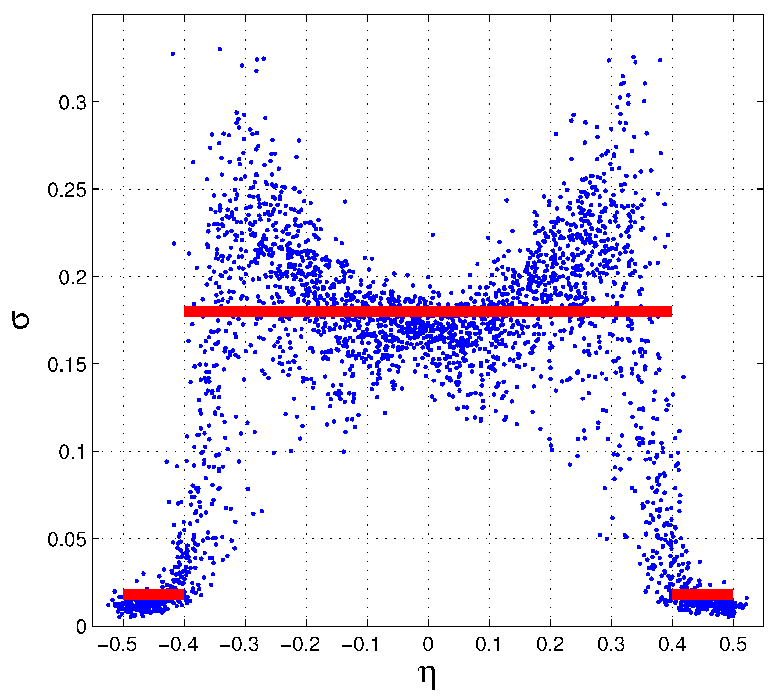
Figure 1. The red lines are the values of σ for the Gaussian model. The blue dots are the effective σ of the schematic model. The dimensions are in strip width ( 63 μ m ). The η -algorithm gives the hit positions, with zero as the strip center.
Instruments 06 00010 g001
Figure 2. The Gaussian model. The blue lines are the γ f -distributions of the standard fit. The red lines are the γ f -distributions of the σ -weighted least squares, they show a linear growth in the resolution. The first distribution is centered on zero, the others are shifted by N 2 identical steps.
Instruments 06 00010 g002
Figure 3. The Gaussian model. Extraction of an approximate linear growth from the standard least squares with the selection of low ψ 2 -values.
Instruments 06 00010 g003
Figure 4. Schematic model. The blue γ f distributions are the standard least squares fits. The red γ f distributions show the linear growth and are produced with the effective σ for each hit.
Instruments 06 00010 g004
Figure 5. Scatter plot of the effective σ as function of the COG 2 ( x g 2 ) scaled to reach an approximate overlap with the COG 2 histogram. More precisely a merged set of red dots corresponding to the blue dots. They are obtained as by-product of the η -algorithm.
Instruments 06 00010 g005
Figure 6. The lucky model. The blue distributions are the standard least squares. The red distributions are the γ f given by the lucky model, very near to those of the schematic model.
Instruments 06 00010 g006
Figure 7. The maximum likelihood evaluations. The blue distributions are the standard least squares. The red distributions are the γ f given by the schematic model, the black distributions are the maximum likelihood evaluations, their empirical PDFs are partially covered by those of the schematic model, however their higher maxima are clearly visible.
Instruments 06 00010 g007
Figure 8. The asterisks are the H G = 1 / ( 2 π Σ D ) the heights of a Gaussian of Σ D as standard deviation. The circles are the maxima of the γ f empirical PDFs. The color code is that of Figure 7.
Instruments 06 00010 g008
Publisher’s Note: MDPI stays neutral with regard to jurisdictional claims in published maps and institutional affiliations.