Article

Regression with Gaussian Mixture ModelsApplied to Track Fitting

by
Rudolf Frühwirth
Institute of High Energy Physics (HEPHY), Austrian Academy of Sciences, Nikolsdorfer Gasse 18, 1050 Wien, Austria
Instruments 2020, 4(3), 25; https://doi.org/10.3390/instruments4030025
Submission received: 28 July 2020 / Revised: 28 August 2020 / Accepted: 28 August 2020 / Published: 31 August 2020

Abstract

:
This note describes the application of Gaussian mixture regression to track fitting with a Gaussian mixture model of the position errors. The mixture model is assumed to have two components with identical component means. Under the premise that the association of each measurement to a specific mixture component is known, the Gaussian mixture regression is shown to have consistently better resolution than weighted linear regression with equivalent homoskedastic errors. The improvement that can be achieved is systematically investigated over a wide range of mixture distributions. The results confirm that with constant homoskedastic variance the gain is larger for larger mixture weight of the narrow component and for smaller ratio of the width of the narrow component and the width of the wide component.

1. Introduction

In the data analysis of high-energy physics experiments, and particularly in track fitting, Gaussian models of measurements errors or Gaussian models of stochastic processes such as multiple Coulomb scattering and energy loss of electrons by bremsstrahlung may turn out to be too simplistic or downright invalid. In these circumstances Gaussian mixture models (GMMs) can be used in the data analysis to model outliers or tails in position measurements of tracks [1,2], to model the tails of the multiple Coulomb scattering distribution [3,4], or to approximate the distribution of the energy loss of electrons by bremsstrahlung [5]. In these applications it is not known to which component an observation or a physical process corresponds, and it is up to the track fit via the Deterministic Annealing Filter or the Gaussian-sum Filter to determine the association probabilities [6,7,8,9]. The standard method for concurrent maximum-likelihood estimation of the regression parameters and the association probabilities is the EM algorithm [10,11].
In a typical tracking detector such as a silicon strip tracker, the spatial resolution of the measured position is not necessarily uniform across the sensors and depends on the crossing angle of the track and on the type of the cluster created by the particle. By a careful calibration of the sensors in the tracking detector a GMM of the position measurements can be formulated, see [12,13,14]. In such a model the component from which an observation is drawn is known. This can significantly improve the precision of the estimated regression/track parameters with respect to weighted least-squares, as shown below.
This introduction is followed by a recapitulation of weighted regression in linear and nonlinear Gaussian models in Section 2, both for the homoskedastic and for the heteroskedastic case. Section 3 introduces the concept of Gaussian mixture regression (GMR) and derives some elementary results on the covariance matrices of the estimated regression parameters. Section 4 presents the results of simulation studies that apply GMR to track fitting in a simplified tracking detector. The gain in precision that can be obtained by using a GMM rather than a simple Gaussian model strongly depends on the shape of the mixture distribution of the position errors. This shape can be described concisely by two characteristic quantities: the weight p of the wider component, and the ratio r of the smaller over the larger standard deviation. The study covers a wide range of p and r and shows the gain as a function of the number of measurements within a fixed tracker volume. It also investigates the effect of multiple Coulomb scattering on the gain in precision. Finally, Section 5 gives a summary of the results and discusses them in context of the related work in [12,13,14].

2. Linear Regression in Gaussian Models

This section briefly recapitulates the properties of linear Gaussian regression models and the associated estimation procedures.

2.1. Linear Gaussian Regression Models

The general linear Gaussian regression model (LGRM) has the following form:
y = X θ + c + ϵ , with V = Var [ ϵ ] and ϵ N ( 0 , V ) ,
where y is the vector of observations, θ is the vector of unknown regression parameters, X is the known model matrix, c is a known vector of constants, and ϵ is the vector of observation errors, distributed according to the multivariate normal distribution N ( 0 , V ) with mean 0 and covariance matrix V . In the following it is assumed that dim ( y ) dim ( θ ) and rank ( X ) = dim ( θ ) .
If the covariance matrix V is diagonal, i.e., the observation errors are independent, two cases are distinguished in the literature. The errors in Equation (1) and the model are called homoskedastic, if V is a multiple of the identity matrix:
V = σ 2 · I .
Otherwise, the errors in Equation (1) and the model are called heteroskedastic. If V is not diagonal, the observation errors are correlated, in which case the the model is called homoskedastic if all diagonal elements are identical, and heteroskedastic otherwise.

2.2. Estimation, Fisher Information Matrix and Efficiency

In least-squares (LS) estimation, the regression parameters θ are estimated my minimizing the following quadratic form with respect to θ :
S ( θ ) = ( y c X θ ) T G ( y c X θ ) , with G = V 1 .
Setting the gradient of S ( θ ) to zero gives the LS estimate θ ^ of θ , and linear error propagation yields its covariance matrix C ^ :
θ ^ = ( X T G X ) 1 X T G ( y c ) , C ^ = Var [ θ ^ ] = ( X T G X ) 1 .
It is easy to see that θ ^ is an unbiased estimate of the unknown parameter θ .
In the LGRM, the LS estimate is equal to the maximum-likelihood (ML) estimate. The likelihood function L ( θ ) and its logarithm ( θ ) are given by:
L ( θ ) = C · exp 1 2 ( y c X θ ) T G ( y c X θ ) ,
( θ ) = log ( C ) 1 2 ( y c X θ ) T G ( y c X θ ) , C R .
The gradient ( θ ) is equal to:
( θ ) = ( θ ) θ = ( y c X θ ) T G X ,
and its matrix of second derivatives, the Hesse matrix H ( θ ) is equal to:
H ( θ ) = 2 ( θ ) θ 2 = X T G X .
Setting the gradient to zero yields the ML estimate, which is identical to the LS estimate.
Under mild regularity conditions, the covariance matrix of an unbiased estimator cannot be smaller than the inverse of the Fisher information matrix; this is the famous Cramér-Rao inequality [15]. The (expected) Fisher information matrix I ( θ ) of the parameters θ is defined as the negative expectation of the Hesse matrix of the log-likelihood function:
I ( θ ) = E [ ( θ ) ] = X T G X .
Equation (4) shows that in the LGRM the covariance matrix of the LS/ML estimate is equal to the inverse of the Fisher information matrix. The LS/ML estimator is therefore efficient: no other unbiased estimator of θ can have a smaller covariance matrix.

2.3. Nonlinear Gaussian Regression Models

In most applications to track fitting, the track model that describes the dependence of the observed track positions on the track parameters is nonlinear. The general nonlinear regression Gaussian model has the following form:
y = f ( θ ) + ϵ , with ϵ N ( 0 , V ) ,
where f ( θ ) is a nonlinear smooth function. The estimation of θ usually proceeds via Taylor expansion of the model function to first order:
y f ( θ 0 ) + X ( θ θ 0 ) + ϵ = X θ + c + ϵ , with
X = f θ θ 0 , c = f ( θ 0 ) X θ 0 ,
where θ 0 is a suitable expansion point and the Jacobian X is evaluated at θ 0 . The estimate θ 1 is obtained according to Equation (4). The model function is then re-expanded at θ 1 , and the procedure is iterated until convergence.

3. Linear Regression in Gaussian Mixture Models

If the observation errors do not follow a normal distribution, the Gaussian linear model can be generalized to a GMM, which is more flexible, but still retains some of the computational advantages of the Gaussian model. Applications of Gaussian mixtures can be traced back to Karl Pearson more than a century ago [16]. In view of the applications in Section 4, the following discussion is restricted to Gaussian mixtures with two components with identical means. The probability density function (PDF) g ( y ) of such a mixture has the following form:
g ( y ) = p · φ ( y ; μ , σ 1 ) + ( 1 p ) · φ ( y ; μ , σ 0 ) , 0 < p < 1 , σ 0 < σ 1 ,
where φ ( y ; μ , σ ) denotes the normal PDF with mean μ and variance σ 2 . The Gaussian mixture (GM) with this PDF is denoted by GM ( p , μ , σ 1 , σ 0 ) . The component with index 0 is called the narrow component, the component with index 1 is called the wide component in the following.

3.1. Homoskedastic Mixture Models

We first consider the following linear GMM:
y = X θ + c + ϵ , with ϵ i GM ( p , 0 , σ 1 , σ 0 ) , i = 1 , , n ,
where n = dim ( y ) . The variance of ϵ i is equal to:
var [ ϵ i ] = σ tot 2 = p · σ 1 2 + ( 1 p ) · σ 0 2 , i = 1 , , n ,
and the joint covariance matrix of ϵ is equal to
V = Var [ ϵ ] = σ tot 2 · I .
As the total variance is the same for all i, the GMM is called homoskedastic. By using just the total variances, it can be approximated by a homoskedastic LGRM, and the estimation of the regression parameters proceeds as in Equation (4), which can be simplified to:
θ ˇ = ( X T X ) 1 X T ( y c ) , C ˇ = σ tot 2 · ( X T X ) 1 .
If the association of the observations to the components is known, it can be encoded in a binary vector z Z = { 0 , 1 } n , where z i = j indicates the component with variance σ j 2 , for i = 1 , , n . In the case of independent draws from the mixture PDF in Equation (13), the z i are independent Bernoulli variables with P ( 1 ) = p , P ( 0 ) = 1 p . The probability of z = ( z 1 , , z n ) is therefore equal to:
P ( z ) = i = 1 n p z i ( 1 p ) 1 z i = p k ( 1 p ) n k , with k = i = 1 n z i .
Conditional on the known associations z , the model can be interpreted as a heteroskedastic LGRM with a diagonal covariance matrix V z :
V z = Var [ ϵ | z ] = diag ( σ z 1 2 , , σ z n 2 ) , and G z = V z 1 .
It follows from the binomial theorem that:
V = z Z P ( z ) · V z .
The GMR is thus a mixture of heteroskedastic Gaussian linear regressions with mixture weights P ( z ) , z Z . In each of the heteroskedastic LGRMs the regression parameters are estimated by:
θ ^ z = ( X T G z X ) 1 X T G z ( y c ) , C ^ z = ( X T G z X ) 1 .
Conditional on z , the estimator is normally distributed with mean θ and covariance matrix C ^ z , and therefore unbiased and efficient. The unconditional distribution of θ ^ is obtained by summing over all z with weights P ( z ) . Its density therefore reads:
f ( θ ^ ) = z Z P ( z ) · φ ( θ ^ ; θ , C ^ z ) ,
where φ ( θ ^ ; θ , C ^ z ) is the multivariate normal density of θ ^ with mean θ and covariance matrix C ^ z . θ ^ is therefore unbiased, and its covariance matrix is obtained by summing over the 2 n possible values of z with weights P ( z ) :
C ^ = z Z P ( z ) · C ^ z .
The unconditional estimator has minimum variance among all estimators that are conditionally unbiased for all z Z , as shown by the following theorem.
Theorem 1.
Let θ ˜ be an estimator of θ with E [ θ ˜ | z ] = θ for all z Z . Then its covariance matrix C ˜ is not smaller than C ^ in the Loewner partial order:
C ^ C ˜ .
Proof. 
As E [ θ ˜ | z ] = θ , C ˜ can be written in the following form:
C ˜ = z Z P ( z ) · C ˜ z , with C ˜ z = Var [ θ ˜ | z ] .
As θ ^ z is efficient conditional on z and θ ˜ | z is conditionally unbiased, it follows that
C ^ z = Var [ θ ^ | z ] Var [ θ ˜ | z ] = C ˜ z , z Z .
Summing over all z with weights P ( z ) proves the theorem. □
Collorary. 
C ^ C ˇ , with equality if p { 0 , 1 } .
Proof. 
As E [ θ ˇ | z ] = θ for all z , the estimator θ ˇ fulfills the premise of the theorem. Its conditional covariance matrix is obtained by linear error propagation:
C ˇ z = Var [ θ ˇ | z ] = ( X T X ) 1 X T V z X ( X T X ) 1 .
As θ ^ | z is efficient, C ^ z C ˇ z and C ^ C ˇ . If p { 0 , 1 } , V z is homoskedastic and C ^ z = C ˇ z = σ tot 2 · ( X T X ) 1 . □
The effective improvement in precision of the heteroskedastic estimator θ ^ w.r.t.regarding to the homoskedastic estimator θ ˇ is difficult to quantify by simple formulas, but easy to assess by simulation studies. The results of three such studies in the context of track fitting are presented in Section 4.1, Section 4.2 and Section 4.3, respectively.

3.2. Heteroskedastic Mixture Models

The GMM in Equation (14) can be further generalized to the heteroskedastic case, where the mixture parameters depend on i:
y = X θ + c + ϵ , with ϵ i GM ( p i , 0 , σ i , 1 , σ i , 0 ) , i = 1 , , n .
The joint covariance matrix of ϵ is now diagonal with
V = Var [ ϵ ] = diag ( σ 1 , tot 2 , , σ n , tot 2 ) , with
σ i , tot 2 = p i · σ i , 1 2 + ( 1 p i ) · σ i , 0 2 , i = 1 , , n .
The approximating LGRM that uses just the total variances is now heteroskedastic with covariance matrix V . The corresponding estimator θ ˇ with its covariance matrix C ˇ is computed as in Equation (4).
Conditional on the associations coded in z , the covariance matrix V z now reads:
V z = Var [ ϵ | z ] = diag ( σ 1 , z 1 2 , , σ n , z n 2 ) .
As in Section 3.1, the unconditional covariance matrix C ^ is the weighted sum of the conditional covariance matrices C ^ z :
C ^ = z Z P ( z ) · C ^ z , with P ( z ) = i = 1 n p i z i ( 1 p i ) 1 z i .
It can be proved as before that C ^ C ˇ .
In the application to track fitting, heteroskedastic mixture models can be useful in non-uniform tracking detectors, in which the mixture model obtained by the calibration depends on the layer or on the sensor or on the possible cluster types.
A nonlinear GMM can be approximated by a linear GMM in the same way as a nonlinear Gaussian model can be approximated by a LGRM, see Section 2.3.

4. Track Fitting with Gaussian Mixture Models

4.1. Simulation Study with Straight Tracks

The setting of the first simulation study is a toy detector that consists of n equally spaced sensor planes in the interval from 0 cm to 115 cm . The track model is a straight line in the ( x , y ) -plane. No material effects are simulated. The track position is recorded in each sensor plane, with a position error generated from a Gaussian mixture, see Equation (13). The total variance in each layer is equal to σ tot 2 = ( 0.005 cm ) 2 , corresponding to a standard deviation of σ tot = 0.005 cm . As the main objective of the simulation study is the comparison of the homoskedastic estimator of Equation (17) with the heteroskedastic estimator of Equation (21), the actual value of σ tot 2 is irrelevant.
10 5 tracks were generated for each of 20 combinations of p and r = σ 0 / σ 1 : p = 0.6 , 0.7 , 0.8 , 0.9 ; r = 0.1 , 0.2 , 0.3 , 0.4 , 0.5 . The corresponding values of σ 1 and σ 0 are collected in Table 1. The number n of planes varied from 3 to 20. For each pair ( p , r ) and each value of n the exact covariance matrix was computed according to Equation (23).
The track parameters were chosen as the intercept d and the slope k. All tracks were fitted with the homoskedastic and with the heteroskedastic error model. Figure 1 shows the estimated standard deviation (rms) of both fits, along with the exact values, for the intercept d and the slope k, with p = 0.8 , r = 0.2 in the range 3 n 20 . The standard deviations of the heteroskedastic fit are not only smaller, but also fall at a faster rate than the ones of the homoskedastic fit, i.e., faster than 1 / n . The agreement between the estimated and the exact standard deviations is excellent.
Figure 2 shows the relative standard deviation (heteroskedastic rms over homoskedastic rms) for the slope k and all 20 combinations of p and r. The corresponding plot for the intercept d looks very similar. A clear trend can be observed: the ratio gets smaller with decreasing p and with decreasing r. The largest improvement is therefore seen for p = 0.6 , r = 0.1 , where the probability of very precise measurements ( r = 0.1 ) is the largest ( 1 p = 0.4 ).
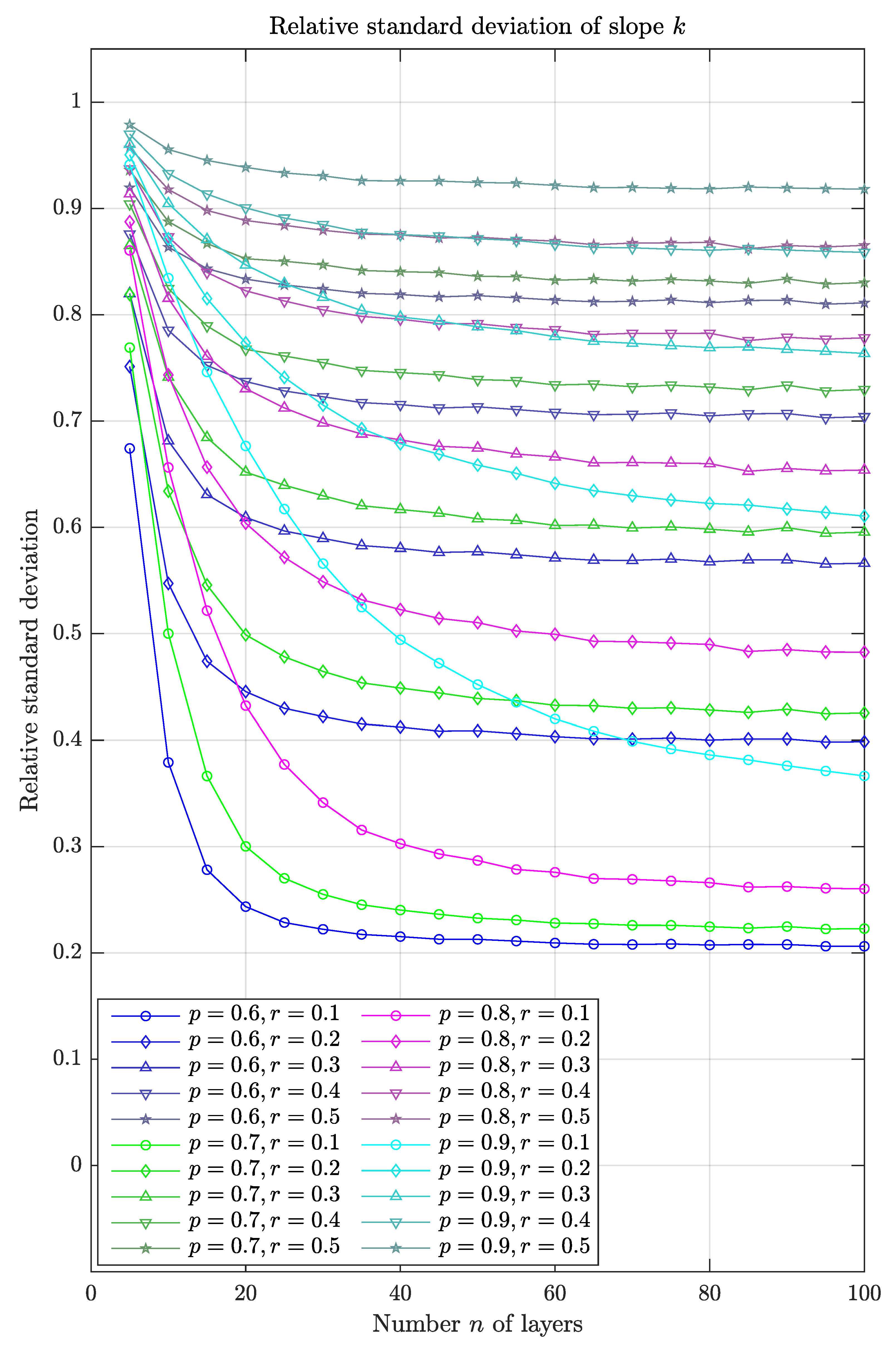
For large values of n the ratio curves approach a constant level, because asymptotically both rms values fall at the same rate, namely 1 / n , see Figure 3. In the experimentally relevant region 15 n 20 the ratio is already close to its lower limit in most, but not all, cases. In these cases, the superior performance of the heteroskedastic fit is fully exploited, and adding more measurements yields little further improvement. The exception is the case p = 0.9 , where the limit is reached much later, at n = 200 in the extreme case.

4.2. Simulation Study with Circular Tracks

The setting of the second simulation study is a toy detector that consists of n equally spaced concentric cylinders with radii in the interval [ R min , R max ] , with R min = 10 , R max = 100 cm . The track model is a helix through the origin. Only the parameters in the bending plane ( ( x , y ) -plane) are estimated. The track parameters are: Φ , the azimuth of the track position at R = R min ; ϕ , the azimuth of the track direction at R = R min ; and κ , the curvature of the circle.
10 6 tracks were generated for each of the same 20 combinations of p and r = σ 0 / σ 1 as in Section 4.1. The track position in the bending plane was recorded in each cylinder, with a position error generated from the Gaussian mixtures in Table 1. Each sample of 10 6 tracks consists of 10 subsamples with circles of 10 different radii, namely ρ / cm = 100 , 200 , , 1000 . The number n of planes varied from 3 to 20.
As the track model is nonlinear, estimation was performed according to the procedure in Section 2.3. All tracks were fitted with the homoskedastic and with the heteroskedastic error model, and for each pair ( p , r ) and each value of n the exact covariance matrix was computed according to Equation (23). Figure 4 shows the estimated standard deviation (rms) of both fits, along with the exact values, for Φ , ϕ and κ , with p = 0.8 , r = 0.2 in the range 3 n 20 . The standard deviations of the heteroskedastic fit are not only smaller, but also fall at a faster rate than the ones of the homoskedastic fit, i.e., faster than 1 / n . The agreement between the estimated and the exact standard deviations is again excellent.
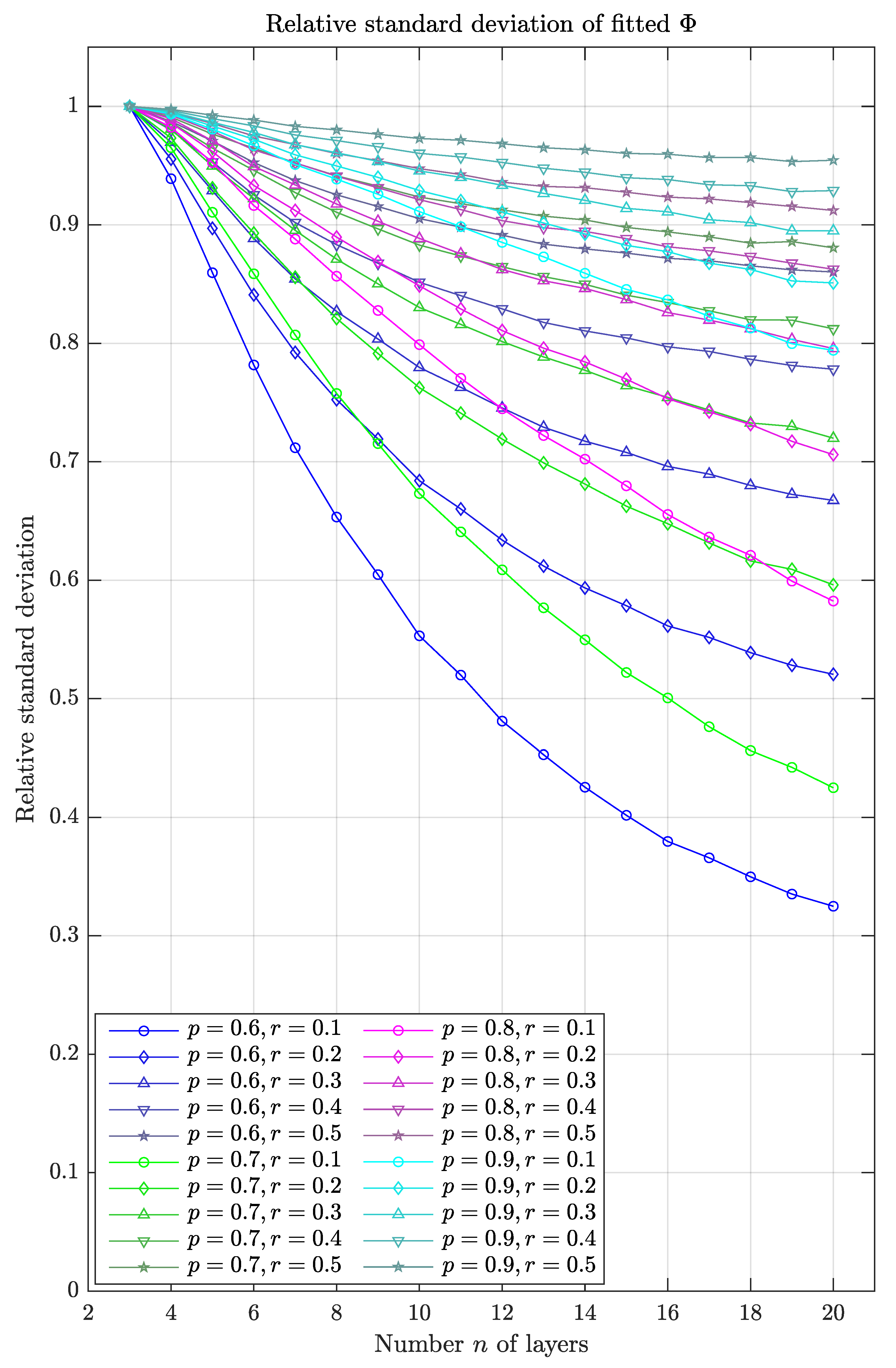
Figure 5, Figure 6 and Figure 7 show the relative standard deviation for the three track parameters and all 20 combinations of p and r. Because of the large correlation between ϕ and κ , Figure 6 and Figure 7 are virtually identical. The same trend as before can be observed: the ratio gets smaller with decreasing p and with decreasing r. The largest improvement is again seen for p = 0.6 , r = 0.1 , where the probability of very precise measurements ( r = 0.1 ) is the largest ( 1 p = 0.4 ). Compared to the results of the straight-line fits, the gain in precision is somewhat smaller.

4.3. Simulation Study with Circular Tracks and Multiple Scattering

The third study investigates the effect of multiple Coulomb scattering (MCS) on the results presented in the previous subsection. To this end, every layer of the toy detector is assumed to have a thickness of 1% of a radiation length. The simulation and the reconstruction of the tracks is modified accordingly, see for example [17].
10 5 tracks were generated for each of four values of the transverse momentum, i.e., p T = 10 , 20 , 50 , 100 GeV / c and for each of the 20 combinations of p and r = σ 0 / σ 1 as in Section 4.2. The dip angle of the tracks was set to λ = π / 4 . The track position in the bending plane was recorded in each cylinder, with a position error generated from the Gaussian mixtures in Table 1 plus a random deviation due to MCS. The number n of planes varied from 3 to 20.
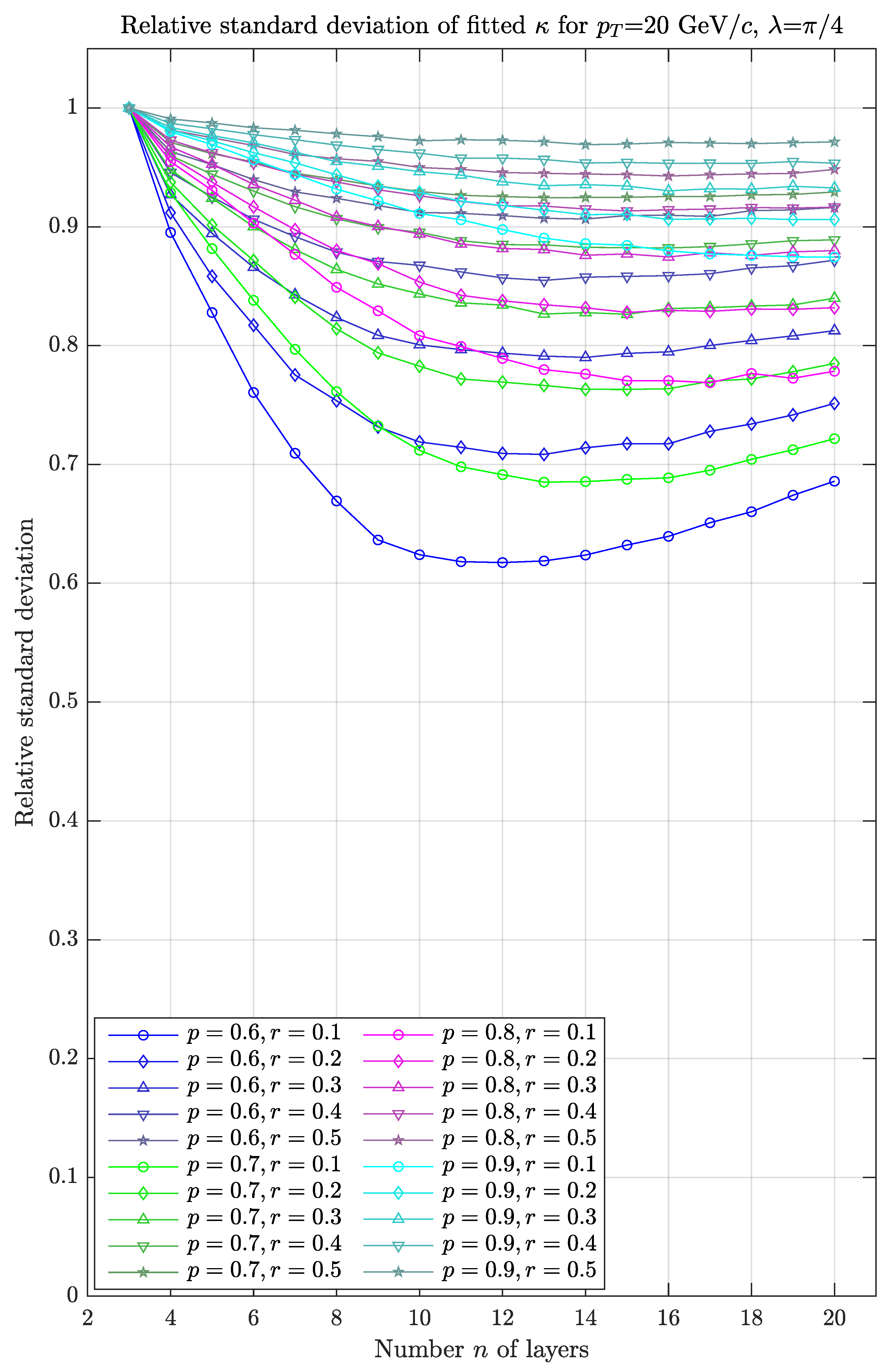
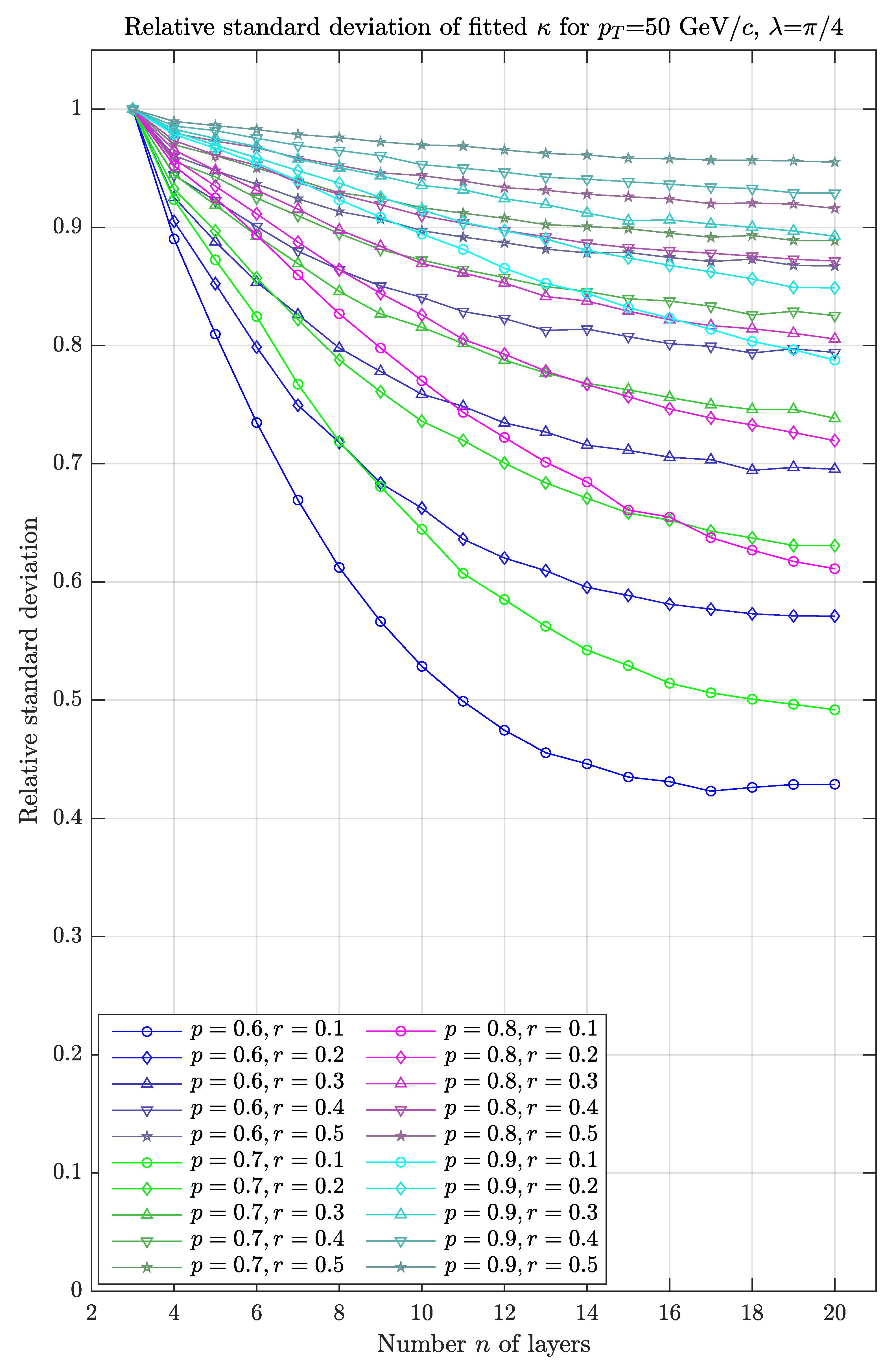
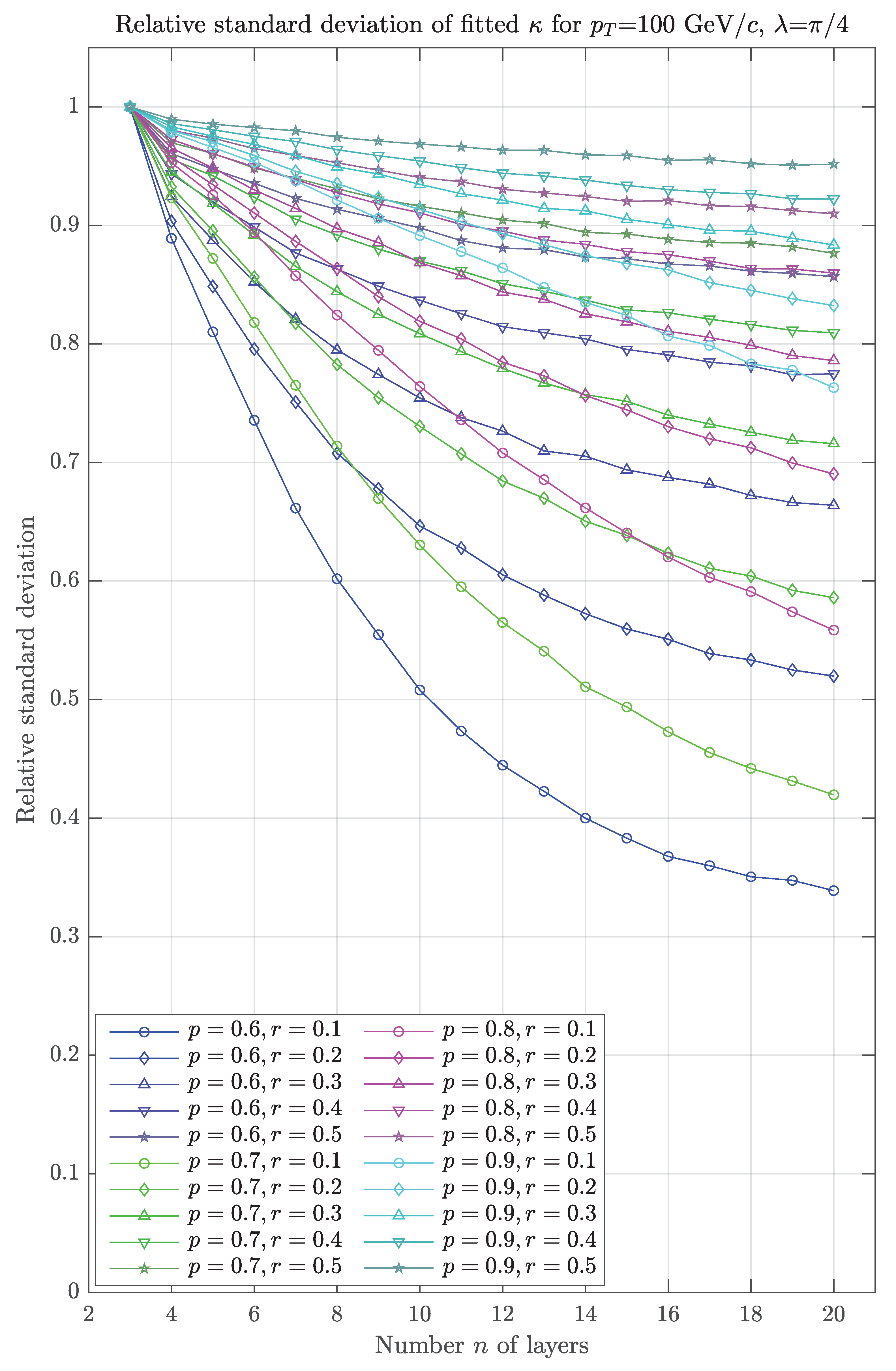
It is to be expected that the benefit provided by the heteroskedastic regression is diminished by the introduction of MCS. This is confirmed by the results in Figure 8, Figure 9, Figure 10 and Figure 11, which show the relative standard deviation of the curvature κ for the four values of p T and the 20 combinations of p and r. Although the gain in precision of the heteroskedastic estimator is rather poor for the lowest value of p T , see Figure 8, it steadily improves with increasing p T and approaches the optimal level for the highest value of p T , see Figure 7 and Figure 11.

5. Summary and Conclusions

We have evaluated the gain in precision that can be achieved by GMR in track fitting using a mixture model of position errors rather than a simple Gaussian model with an average resolution. The results, both with straight and with circular tracks, show the expected behavior: the gain rises if the mixture weight (proportion) of the narrow component becomes larger, and it rises when the ratio of the width of the narrow component and the width of the wide component becomes smaller. Unsurprisingly, the gain is negatively affected by MCS, depending on the track momentum and on the amount of material.
It is also instructive to look at the results in the light of the findings reported in [12,13,14], in particular the claim that the heteroskedastic regression, which is in fact the GMR described here, achieves a linear growth of the resolution with the number n of detecting layers, instead of the usual n behavior [13]. A glance at Figure 3 shows that in fact the heteroskedastic standard deviations initially fall faster than the homoskedastic ones, i.e., faster than 1 / n . Eventually, however, the relative standard deviations level out at a constant ratio, showing that asymptotically both standard deviations obey the expected 1 / n mode of falling with n. The observation reported in [13] is clearly a small-sample effect, which—in contrast to most other cases—is very significant in the mixture with p = 0.8 , r = 0.1 , the one assumed in [13]. Fortunately, it is in the range of n that is relevant for realistic tracking detectors, i.e., somewhere between 5 and 20 for a silicon tracker. It seems therefore absolutely worthwhile to optimize the local reconstruction and error calibration of the position measurements as far as possible.

Funding

This research received no external funding.

Acknowledgments

I thank Gregorio Landi for interesting and instructive discussions. I also thank the anonymous reviewers for valuable comments and corrections, and in particular for suggesting to investigate the effects of multiple Coulomb scattering.

Conflicts of Interest

The author declares no conflict of interest.

Abbreviations

The following abbreviations are used in this manuscript:
GMGaussian Mixture
GMMGaussian Mixture Model
GMRGaussian Mixture Regression
LGRMLinear Gaussian Regression Model
LSLeast-Squares
MCSMultiple Coulomb Scattering
PDFProbability Density Function

References

  1. Frühwirth, R. Track fitting with non-Gaussian noise. Comput. Phys. Commun. 1997, 100, 1. [Google Scholar] [CrossRef] [Green Version]
  2. Frühwirth, R.; Strandlie, A. Track fitting with ambiguities and noise: A study of elastic tracking and nonlinear filters. Comput. Phys. Commun. 1999, 120, 197. [Google Scholar] [CrossRef]
  3. Frühwirth, R.; Regler, M. On the quantitative modelling of core and tails of multiple scattering by Gaussian mixtures. Nucl. Instrum. Meth. Phys. Res. A 2001, 456, 369. [Google Scholar] [CrossRef]
  4. Frühwirth, R.; Liendl, M. Mixture models of multiple scattering: Computation and simulation. Comput. Phys. Commun. 2001, 141, 230. [Google Scholar] [CrossRef]
  5. Frühwirth, R. A Gaussian-mixture approximation of the Bethe-Heitler model of electron energy loss by bremsstrahlung. Comput. Phys. Commun. 2003, 154, 131. [Google Scholar] [CrossRef]
  6. Adam, W.; Frühwirth, R.; Strandlie, A.; Todorov, T. Reconstruction of electrons with the Gaussian-sum filter in the CMS tracker at the LHC. J. Phys. G Nucl. Part. Phys. 2005, 31, N9. [Google Scholar] [CrossRef] [Green Version]
  7. Strandlie, A.; Frühwirth, R. Reconstruction of charged tracks in the presence of large amounts of background and noise. Nucl. Instrum. Meth. Phys. Res. A 2006, 566, 157. [Google Scholar] [CrossRef]
  8. The ATLAS Collaboration. Improved Electron Reconstruction in ATLAS Using the Gaussian Sum Filter-Based Model for Bremsstrahlung; Technical Report ATLAS-CONF-2012-047; CERN: Geneva, Switzerland, 2012. [Google Scholar]
  9. Strandlie, A.; Frühwirth, R. Track and vertex reconstruction: From classical to adaptive methods. Rev. Mod. Phys. 2010, 82, 1419. [Google Scholar] [CrossRef]
  10. Dempster, A.P.; Laird, N.M.; Rubin, D.B. Maximum likelihood from incomplete data via the EM algorithm. J. Royal Stat. Soc. Ser. B 1977, 39, 1. [Google Scholar]
  11. Borman, S. The Expectation Maximization Algorithm—A Short Tutorial; Technical Report; University of Utah: Salt Lake City, UT, USA, 2004; Available online: tinyurl.com/BormanEM (accessed on 30 August 2020).
  12. Landi, G.; Landi, G. Optimizing Momentum Resolution with a New Fitting Method for Silicon-Strip Detectors. Instruments 2018, 2, 22. [Google Scholar] [CrossRef] [Green Version]
  13. Landi, G.; Landi, G. Beyond the N Limit of the Least Squares Resolution and the Lucky Model. 2018. Available online: http://xxx.lanl.gov/abs/1808.06708 (accessed on 20 August 2020).
  14. Landi, G.; Landi, G. The Cramer–Rao Inequality to Improve the Resolution of the Least-Squares Method in Track Fitting. Instruments 2020, 4, 2. [Google Scholar] [CrossRef] [Green Version]
  15. Kendall, M.; Stuart, A. The Advanced Theory of Statistics, 3rd ed.; Charles Griffin: London, UK, 1973; Volume 2. [Google Scholar]
  16. Pearson, K. Contributions to the mathematical theory of evolution. Phils. Trans. R. Soc. Lond. A 1894, 185. [Google Scholar]
  17. Brondolin, E.; Frühwirth, R.; Strandlie, A. Pattern recognition and reconstruction. In Particle Physics Reference Library Volume 2: Detectors for Particles and Radiation; Fabjan, C., Schopper, H., Eds.; Springer International Publishing: Cham, Switzerland, 2020. [Google Scholar]
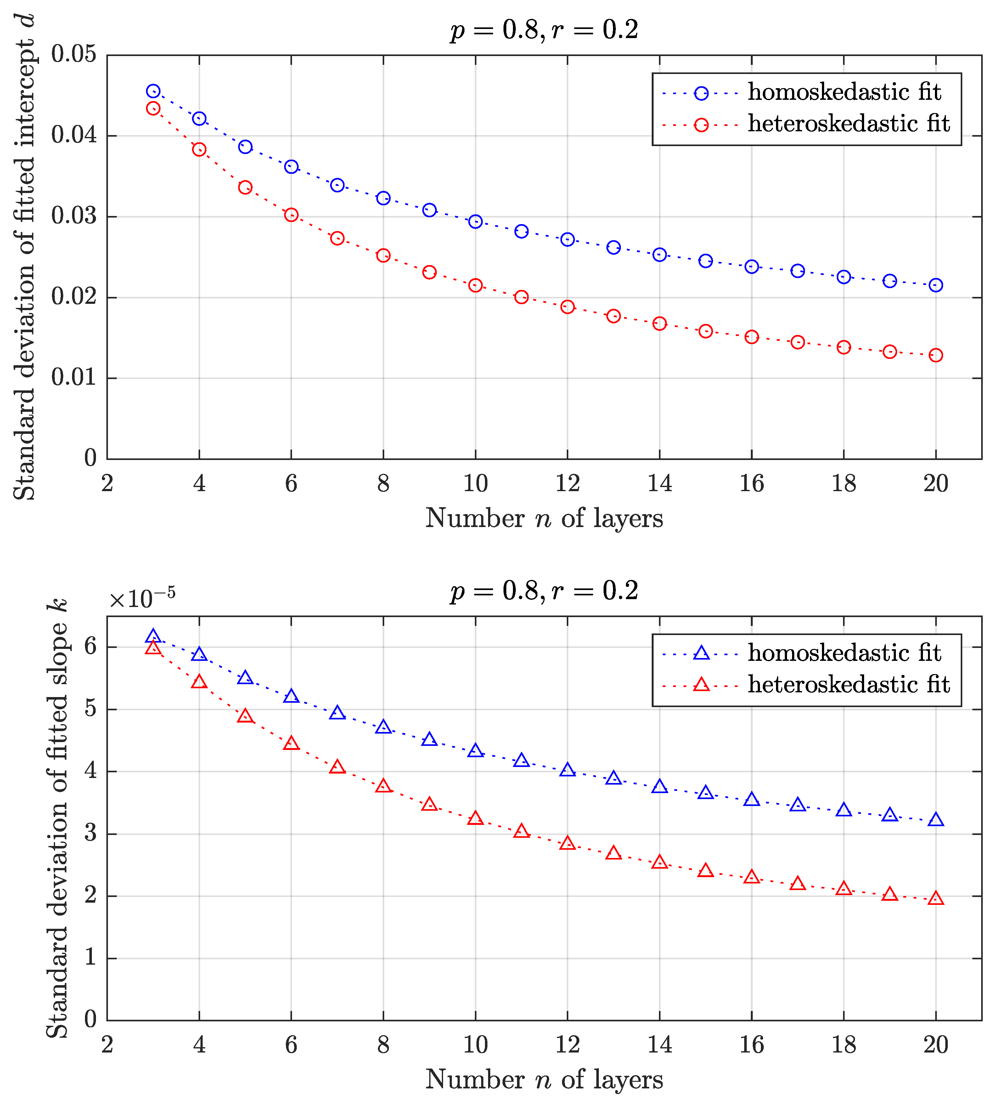
Figure 1. Top: estimated rms and exact standard deviation of the fitted intercept d; bottom: estimated rms and exact standard deviation of the fitted slope k, for p = 0.8 , r = 0.2 in the range 3 n 20 .
Instruments 04 00025 g001
Figure 2. Relative standard deviation (heteroskedastic rms over homoskedastic rms) of the fitted slope k for all 20 combinations of p and r in the range 3 n 20 .
Instruments 04 00025 g002
Figure 3. Relative standard deviation (heteroskedastic rms over homoskedastic rms) of the fitted slope k for all 20 combinations of p and r in the range 5 n 100 .
Instruments 04 00025 g003
Figure 4. Top: estimated rms and exact standard deviation of the fitted angle Φ ; center: estimated rms and exact standard deviation of the fitted angle ϕ ; bottom: estimated rms and exact standard deviation of the fitted curvature κ , for p = 0.8 , r = 0.2 in the range 3 n 20 .
Instruments 04 00025 g004
Figure 5. Relative standard deviation (heteroskedastic rms over homoskedastic rms) of the fitted angle Φ for all 20 combinations of p and r in the range 3 n 20 .
Instruments 04 00025 g005
Figure 6. Relative standard deviation (heteroskedastic rms over homoskedastic rms) of the fitted angle ϕ for all 20 combinations of p and r in the range 3 n 20 .
Instruments 04 00025 g006
Figure 7. Relative standard deviation (heteroskedastic rms over homoskedastic rms) of the fitted curvature κ for all 20 combinations of p and r in the range 3 n 20 .
Instruments 04 00025 g007
Figure 8. Relative standard deviation (heteroskedastic rms over homoskedastic rms) of the curvature κ for p T = 10 , GeV / c , λ = π / 4 and all 20 combinations of p and r in the range 3 n 20 .
Instruments 04 00025 g008
Figure 9. Relative standard deviation (heteroskedastic rms over homoskedastic rms) of the curvature κ for p T = 20 , GeV / c , λ = π / 4 and all 20 combinations of p and r in the range 3 n 20 .
Instruments 04 00025 g009
Figure 10. Relative standard deviation (heteroskedastic rms over homoskedastic rms) of the curvature κ for p T = 50 , GeV / c , λ = π / 4 and all 20 combinations of p and r in the range 3 n 20 .
Instruments 04 00025 g010
Figure 11. Relative standard deviation (heteroskedastic rms over homoskedastic rms) of the curvature κ for p T = 100 , GeV / c , λ = π / 4 and all 20 combinations of p and r in the range 3 n 20 .
Instruments 04 00025 g011
Table 1. Values of σ 1 and σ 0 (in µm) for p = 0.6 , 0.7 , 0.8 , 0.9 and r = 0.1 , 0.2 , 0.3 , 0.4 , 0.5 .
p = 0.6p = 0.7p = 0.8p = 0.9
σ 1 σ 0 σ 1 σ 0 σ 1 σ 0 σ 1 σ 0
r = 0.164.36.459.66.055.85.652.75.3
r = 0.263.712.759.311.955.611.152.610.5
r = 0.362.718.858.617.655.316.652.415.7
r = 0.461.424.557.823.154.821.952.220.9
r = 0.559.729.956.828.454.227.152.026.0