Dielectric-Filled Reentrant Cavity Resonator as a Low-Intensity Proton Beam Diagnostic

Abstract

Measurement of the proton beam current (0.1–40 nA) at the medical treatment facility PROSCAN at the Paul Scherrer Institut (PSI) is performed with ionization chambers. To mitigate the scattering issues and to preserve the quality of the beam delivered to the patients, a non-interceptive monitor based on the principle of a reentrant cavity resonator has been built. The resonator with a fundamental resonance frequency of 145.7 MHz was matched to the second harmonic of the pulse repetition rate (72.85 MHz) of the beam extracted from the cyclotron. This was realized with the help of ANSYS HFSS (High Frequency Structural Simulator) for network analysis. Both, the pickup position and dielectric thickness were optimized. The prototype was characterized with a stand-alone test bench. There is good agreement between the simulated and measured parameters. The observed deviation in the resonance frequency is attributed to the frequency dependent dielectric loss tangent. Hence, the dielectric had to be resized to tune the resonator to the design resonance frequency. The measured sensitivity performances were in agreement with the expectations. We conclude that the dielectric reentrant cavity resonator is a promising candidate for measuring low proton beam currents in a non-destructive manner.

1. Introduction

For any particle accelerator facility, beam diagnostics are important tools to measure beam parameters such as beam current, position, profile, emittance etc. These diagnostic devices can be classified as interceptive monitors such as the ionization chamber, Faraday cup, wire scanner, etc., and non-interceptive monitors such as the beam current transformer, wall current monitor, pick-up, etc. [1]. A number of accelerator facilities using proton or light-ion beams [2] are dedicated to the medical treatment of tumors. At the Paul Scherrer Institut (PSI), the PROSAN facility has been built exactly for this purpose. Its superconducting cyclotron delivers a 250 MeV [3] proton beam. The relevant proton beam parameters are summarized in

Table 1. Properties of extracted beam from COMET [4].

Beam Properties	Units
Extracted beam intensity	<1–1000 nA
Energy spread at extraction ΔE/E	0.15%
Beyond the degrader ΔE/E	0.2% at 230 MeV; 2.5% at 70 MeV
Beam diameter	1–20 mm
Repetition rate	72.85 MHz (T = 13.73 ns)
Pulse length	2 ns

.

At PSI, intensities of proton beam from the 590 MeV (>mA) current transformers are used. However, for beam currents of <1–1000 nA at the therapy facility, the transformers (detection threshold ≈1 μA) cannot be used. Hence, for PROSCAN, planar ionization chambers are predominantly used [5,6] to determine the beam current as an intercepting method [7]. The disadvantages of these measurements are scattering issues, energy loss, and activation in the detector itself [8,9]. In addition, the quality of the beam delivered to patients for radiation therapy is affected by such interceptive monitors.

To mitigate the above effects, a non-interceptive monitor is envisaged to measure beam currents of low magnitude down to 0.1 nA. For such proton beam currents, the use of wall current monitors (detection threshold 100 µA) of resistive and inductive types is restricted due to their limited high frequency response caused by the short-circuiting of the ceramic gap and the necessity to employ electric shielding to prevent parasitic current flows at low frequencies into the resistor or inductor, as they are short-circuited by miscellaneous ground connections [10]. Moreover, since they are assembled azimuthally with 10 to 100 resistors, they are also a source of thermal noise. A cryogenic current comparator with a Superconducting Quantum Interference Device (SQUID) [10] detects extremely small magnetic fields with values in the fT to pT range [11]. They have displayed resolution in the fraction of nA ranges. However, since they are sensitive magnetometers, coupling of the magnetic field is crucial. Also, it is necessary to provide shielding from external field contributions and a highly sensitive SQUID electronics system is essential [12]. Consequently, they are not suited for our measurements. Non-destructive monitors of capacitive type such as button or stripline monitors, which couple to the electric field of the beam, also have limited application due to their inability to sense smaller signal levels with high resolution (measurement resolution −20 μA_rms) and their ability to deform such signals due to horizontal-vertical coupling issues [13]. To compensate for this, the azimuthal coverage has to be increased and this results in complex mechanical realization [9,10].

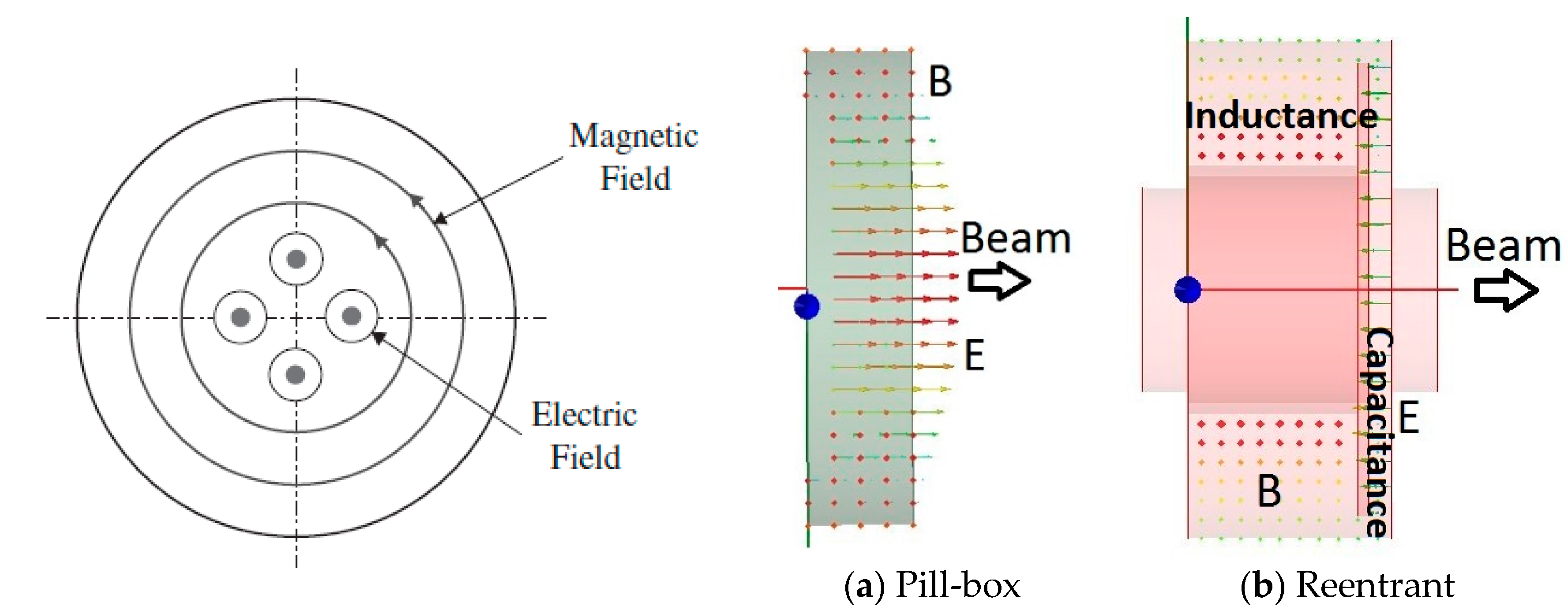
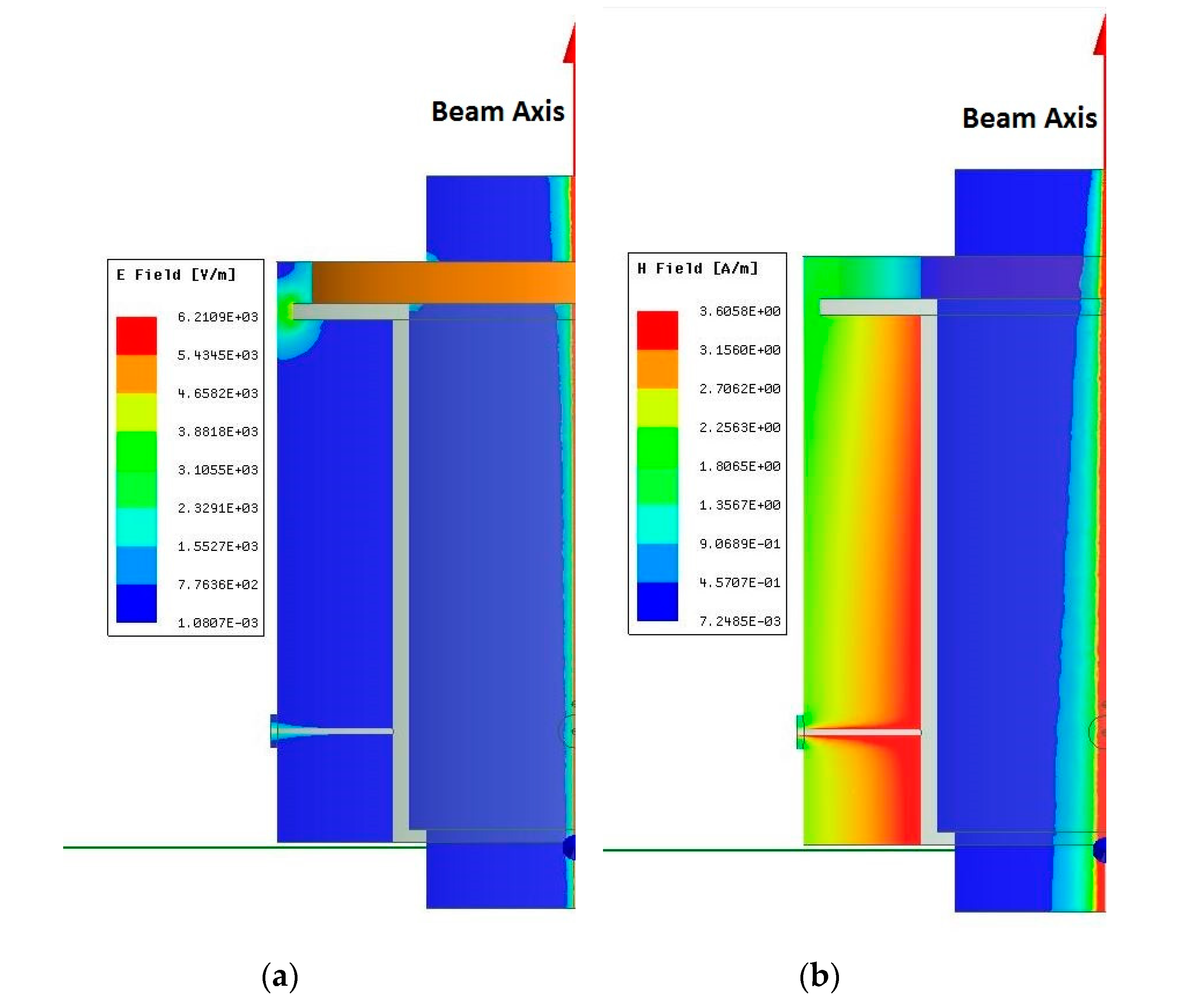
Cavity resonators are in high demand due to their ability to measure small beam currents and their superior sensitivity compared to the other diagnostics mentioned earlier [14]. As shown in Figure 1, the excited fundamental resonance mode (the monopole mode) within the cavity is proportional to the beam current or to total bunch charge [15].

The resonator governed by the outer metallic boundary allows only a discrete set of resonance frequencies with their characteristic field distribution [16]. With a conventional pill-box cavity ($\overrightarrow{\mathrm{E}}$ coupling), these discrete sets of resonance frequencies are separate by a few hundreds of MHz depending on the radius and length. With a reentrant cavity resonator ($\overrightarrow{\mathrm{B}}$ coupling), the higher order modes are damped more strongly compared to the pill-box cavity [17] by sizing the reentrant gap.

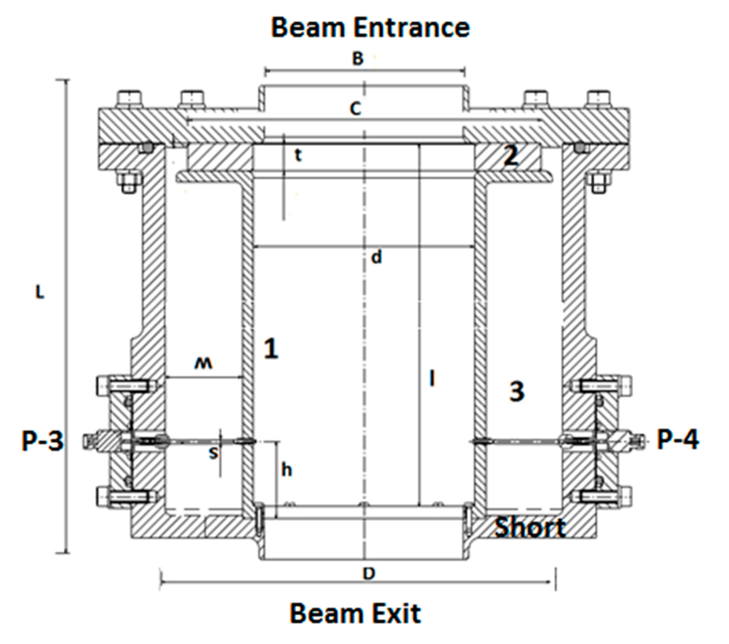
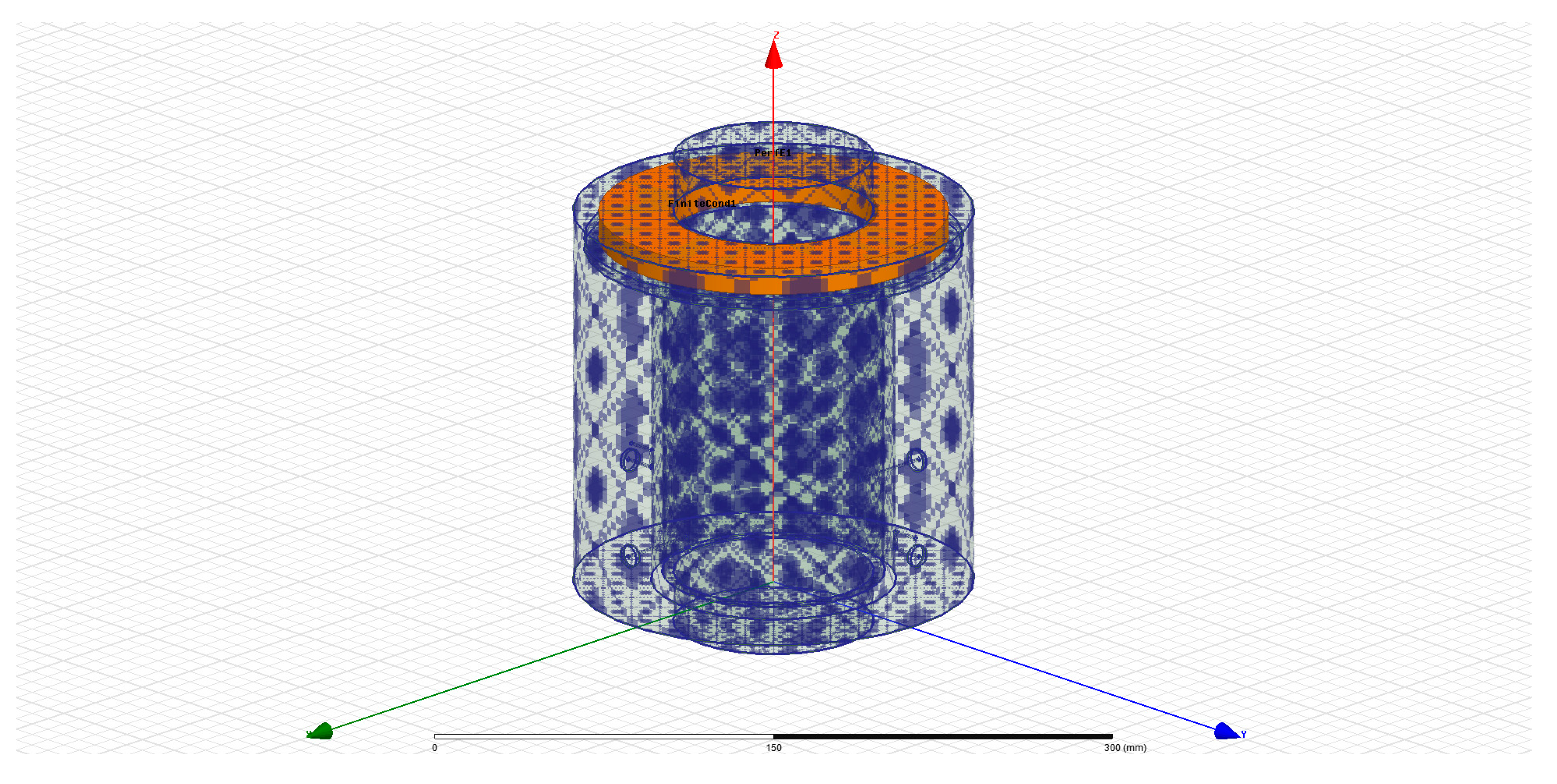
The reentrant cavity resonator designed and built at PSI is a coaxial cavity with a capacitor plane and its wall acting as a distributed inductance. The beam induced wall current (image current) excites the cavity and resonance occurs when the cavity resonance frequency matches a harmonic of the repetition frequency of the beam proton bunches. Compared to the pill-box cavity, the reentrant cavity resonator has a smaller system and it has a lower Q factor for the same resonance frequency [18]. The compactness of the reentrant resonator is essential to save longitudinal space [19]. It also allows simpler and precise manufacturing [20]. A lower Q compared to the pill-box is not only acceptable but it provides less sensitivity to temperature variations that naturally occur in a non-temperature-stabilized environment.

In this paper, we present an option for measuring low proton beam currents by using a dielectric filled reentrant cavity resonator. We explain its working principle, and discuss the resonator design considerations and its advantages. Moreover, we report on the good agreement between simulation and test bench measurements of the prototype. The test bench measurement provides preliminary knowledge about the expected sensitivity and the required signal integration time of the prototype. Since the application of this diagnostic device, either as a safety device or an online monitoring is ruled by the signal integration time, this will be studied in the future with beamline measurements on the prototype.

2. Overview of Working Principle

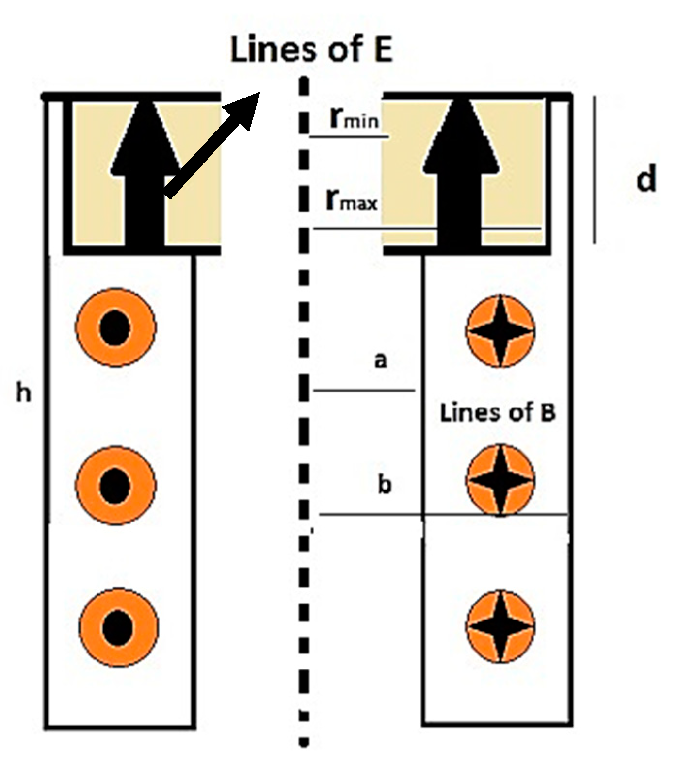
The reentrant cavity resonator’s working principle is very similar to the high frequency resonators described in Feynman’s Lectures [21] (Figure 2). It can be modeled as two connected lump elements, the capacitor plates (${\mathrm{C}}_{\mathrm{gap}}$) and the cavity wall as the inductor (${\mathrm{L}}_{\mathrm{wall}}$), with a resonant angular frequency given then by:

$${\omega }_{\mathrm{o}}=\frac{1}{\sqrt{{\mathrm{L}}_{\mathrm{wall}}·{\mathrm{C}}_{\mathrm{gap}}}},$$

(1)

${\mathrm{C}}_{\mathrm{gap}}$ can be estimated using the standard expression of plate capacitor:

$${\mathrm{C}}_{\mathrm{gap}}=\frac{{\mathsf{\epsilon }}_{\mathrm{r}}{\mathsf{\epsilon }}_{\mathrm{o}}\pi \left({\mathrm{r}}_{\max }^2-{\mathrm{r}}_{\min }^2\right)}{\mathrm{d}},$$

(2)

with ${\mathrm{r}}_{\max }$ and ${\mathrm{r}}_{\min }$ being the outer and inner radius of the plates, and $d$ is the gap between the two plates.

2.1. Transmission Line Analogy

An estimate of the resonator length is attained by performing the calculations within the framework of transmission line theory. This takes into account the coaxial shape of the resonator and the capacitive contribution from the wall itself.

From the expression for the inductance and capacitance of a coaxial transmission line:

$${\mathrm{L}}_{\mathrm{coax}}=\mathrm{h}\frac{\mathsf{\mu }}{2\mathsf{\pi }}\ln \frac{\mathrm{b}}{\mathrm{a}}$$

(3)

$${\mathrm{C}}_{\mathrm{coax}}=\mathrm{h}(2\pi {\mathsf{\epsilon }}_{\mathrm{o}}{\mathsf{\epsilon }}_{\mathrm{r}}/\ln \frac{\mathrm{b}}{\mathrm{a}})$$

(4)

where:

b: the inner radius of the outer conductor

a: the outer radius of the inner conductor

${\mathsf{\epsilon }}_{\mathrm{o}}$: the vacuum permittivity = 8.854 × 10⁻¹² F/m

${\mathsf{\epsilon }}_{\mathrm{r}}$: the relative permittivity of the dielectric of choice

$\mathsf{\mu }$: the permeability, for the vacuum = 4$\pi$ × 10⁻⁷ H/m, and

$\mathrm{h}$: the length of the coaxial line, i.e., the reentrant cavity resonator.

The characteristic impedance of the coaxial line can be expressed as: ${\mathrm{Z}}_0=\sqrt{{\mathrm{L}}_{\mathrm{coax}}/{\mathrm{C}}_{\mathrm{coax}}}$

Using the general expression for a lossless line, the impedance $\mathrm{Z}$ as seen at the input of a coaxial line [22]:

$$\mathrm{Z}={\mathrm{Z}}_0\left[\frac{\raisebox{1ex}{${\mathrm{Z}}_{\mathrm{L}}$}\!\left/ \!\raisebox{-1ex}{${\mathrm{Z}}_0$}\right.+\mathrm{j}.\tan (\mathsf{\beta }\mathrm{h})}{1+\mathrm{j}.\raisebox{1ex}{${\mathrm{Z}}_{\mathrm{L}}$}\!\left/ \!\raisebox{-1ex}{${\mathrm{Z}}_0$}\right..\tan (\mathsf{\beta }\mathrm{h})}\right]$$

(5)

where $\mathsf{\beta }=\frac{2\pi }{\lambda }$ is the wave number, $\mathrm{h}$ is the length of the transmission line, j is the complex imaginary, and ${\mathrm{Z}}_{\mathrm{L}}$ is a load impedance.

In our case, in fact it is a short-circuit line, i.e., Z_L = 0, and the equation (6) can be simplified to:

$${\mathrm{Z}}_{\mathrm{i}}=\mathrm{j}\hspace{0.17em}{\mathrm{Z}}_{\mathrm{o}}\hspace{0.17em}\tan \left(\frac{2\pi \mathrm{h}}{\lambda }\right)$$

(6)

Equation shows that the impedance is inductive for resonator length smaller than λ/4 as it is in the form of an inductive reactance.

Thus, in our case, the resonance is obtained at the frequency for which the gap capacitance C_gap compensates ${\mathrm{Z}}_{\mathrm{i}}$, and replacing the angular frequency ${\mathsf{\omega }}_0$ the corresponding wave length ${\lambda }_0$ and $\mathrm{c}$ the propagation velocity:

$${\mathrm{Z}}_{\mathrm{i}}=-\frac{{\lambda }_0}{\mathrm{j}\hspace{0.17em}2\pi \hspace{0.17em}\mathrm{c}\hspace{0.17em}{\mathrm{C}}_{\mathrm{gap}}}$$

(7)

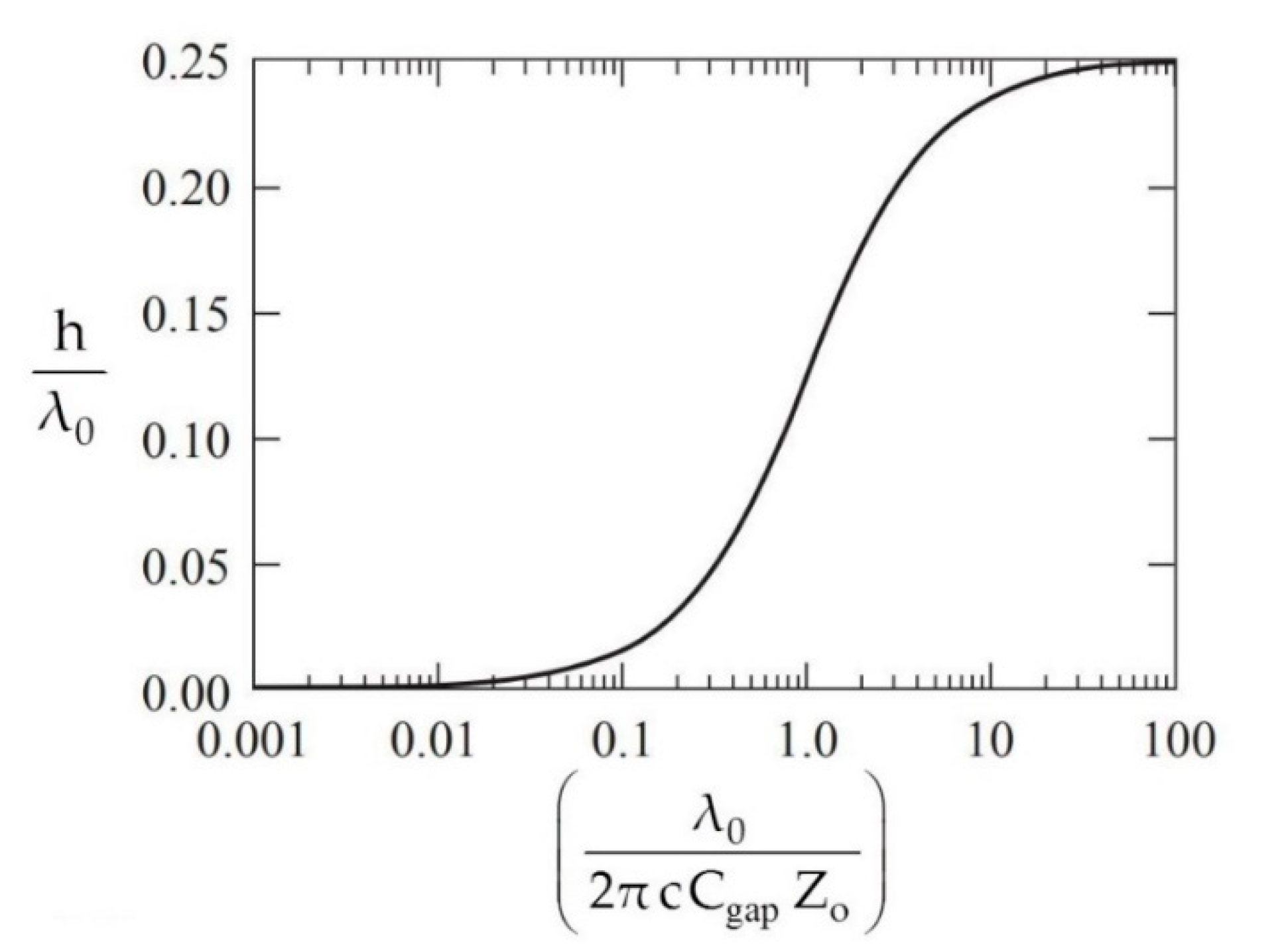
The resonance condition then yields:

$$\frac{2\pi \mathrm{h}}{{\lambda }_0}=\mathrm{t}\mathrm{a}{\mathrm{n}}^{-1}\left(\frac{{\lambda }_0}{2\pi \mathrm{c}{\mathrm{C}}_{\mathrm{gap}}{\mathrm{Z}}_{\mathrm{o}}}\right)$$

(8)

Figure 3 shows the universal tuning curve, which helps in determining the length of the resonator for a given resonance frequency normalized to the quarter-wavelength resonance. For a gap capacitance of 49.4 pF, and a coaxial characteristic impedance of 36 Ω, a free space wavelength corresponding to 2.06 m (corresponding to 145.7 MHz), h is approximately 180 mm. This corresponds to the length, i.e., the length of the inner cylinder + the thickness of the dielectric.

2.2. Q (Quality) Factor

The so-called quality factor Q is used for characterizing the bandwidth and the rate of energy loss of a resonator. It is defined as the ratio between the maximum energy stored in the resonator and the dissipated energy [24,25] and can be expressed as [26]:

$$\mathrm{Q}={\left[\frac{\omega \hspace{0.17em}{\mathrm{W}}_{\max }}{{\mathrm{P}}_{\mathrm{d}}}\right]}_{\omega ={\omega }_{\mathrm{res}}}$$

(9)

where:

${\mathrm{W}}_{\max }$: Maximum energy stored in the resonator

${\mathrm{P}}_{\mathrm{d}}$: Average dissipated power.

The losses that account for the dissipated energy may be located in the cavity itself as internal losses (non-perfectly conducting cavity wall ${\mathrm{P}}_{\mathrm{cond}}$ and lossy dielectrics ${\mathrm{P}}_{\mathrm{d}\mathrm{i}\mathrm{e}\mathrm{l}}$), may be due to the radiated electromagnetic field ${\mathrm{P}}_{\mathrm{r}\mathrm{a}\mathrm{d}}$ or originate from the coupled external circuitry ${\mathrm{P}}_{\mathrm{e}\mathrm{x}}$ (cable, external load) as external losses. The unloaded Q factor ${\mathrm{Q}}_0$ is from the internal losses and the loaded Q factor ${\mathrm{Q}}_{\mathrm{L}}$ takes into account all the possible losses:

$${\mathrm{Q}}_{\mathrm{L}}={\left[\frac{\omega \hspace{0.17em}{\mathrm{W}}_{\mathrm{m}\mathrm{a}\mathrm{x}}}{{\mathrm{P}}_{\mathrm{c}\mathrm{o}\mathrm{n}\mathrm{d}}+{\mathrm{P}}_{\mathrm{d}\mathrm{i}\mathrm{e}\mathrm{l}}+{\mathrm{P}}_{\mathrm{r}\mathrm{a}\mathrm{d}}+{\mathrm{P}}_{\mathrm{e}\mathrm{x}}}\right]}_{\omega ={\omega }_{\mathrm{r}\mathrm{e}\mathrm{s}}}$$

(10)

By assuming the radiated losses are negligible ${\mathrm{P}}_{\mathrm{r}\mathrm{a}\mathrm{d}}$ = 0, we can simplify the above equation to:

$$\frac{1}{{\mathrm{Q}}_{\mathrm{L}}}=\frac{1}{{\mathrm{Q}}_0}+\frac{1}{{\mathrm{Q}}_{\mathrm{e}\mathrm{x}\mathrm{t}}}$$

(11)

If the cavity is used as a beam current diagnostic element, the external connection is usually 50Ω to minimize the reflections on the line. As will be shown in the simulation results, if the external quality factor, i.e., ${\mathrm{Q}}_{\mathrm{e}\mathrm{x}\mathrm{t}}$ is much smaller than ${\mathrm{Q}}_0$, it has the most effect on the loaded Q, i.e., ${\mathrm{Q}}_{\mathrm{L}}$.

When looking at the bandwidth of the resonance system, the Q factor translates to the ratio between the resonance frequency and the bandwidth at −3 dB:

$$\mathrm{Q}=\frac{{\omega }_0}{\Delta {\omega }_{3\mathrm{d}\mathrm{B}}}$$

(12)

2.3. Second Harmonic Matching

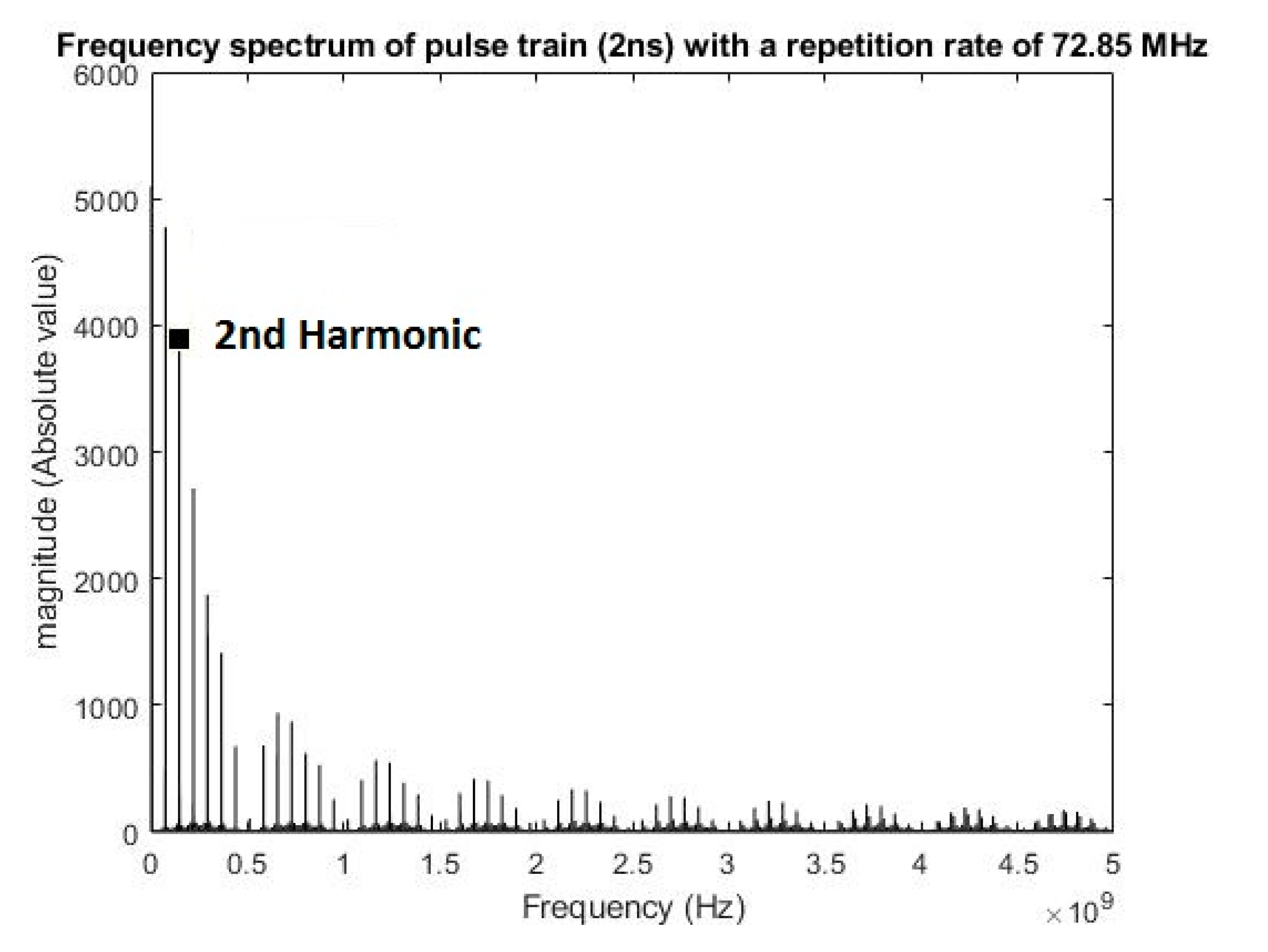
The fundamental resonance frequency of the reentrant cavity resonator is matched to the second harmonic of the 72.85 MHz beam bunch repetition rate to suppress the direct noise of the RF frequency. This frequency harmonic has been selected because of the expected Fourier spectrum (Figure 4) of the pulses produced by the proton bunches. Indeed, it first contains more energy compared to higher frequency components, and it is also less dependent on the exact shape of the measured pulse signals produced by the proton bunches compared to higher harmonics. The fundamental component has been disregarded because of the direct perturbations produced by the cyclotron accelerating cavities.

The measurements were performed at one frequency, i.e., 145.7 MHz, to deliver a signal that is proportional to the beam current. By assuming, for the sake of simplification, a square pulse for the proton bunch shape, the various Fourier components X_n of the signal are directly proportional to the beam current itself [27]:

$$X_n=\frac{A\Delta }{T}\mathrm{sinc}(n\Delta /T)$$

(13)

where A is the amplitude of the beam pulse, Δ is the beam pulse length, T is the period of the repetition rate, n is the harmonic. Since the product AΔ is proportional to the charges contained in 1 pulse, AΔ/T is proportional to the beam current.

3. Resonator Design

ANSYS HFSS was used as the simulation tool [28] for the design of the resonator as the solution is derived from the differential form of Maxwell’s equation [29]. The dielectric filled reentrant cavity forming a coaxial line with the beam pipe has three main mechanical parts, as shown in Figure 5. Part 1 is the beam tube, Part 2 is the dielectric gap filled with Macor [30], and Part 3 is the coaxial extension which is short circuited at the downstream. This design provides mechanical simplicity and allows for precise machining due to its cylindrical symmetry. The cavity is made of aluminum; the dielectric is made of the ceramic, Macor, which was selected for its easy machinability. The reentrant cavity without the Macor will have a resonance at 225.0 MHz. Insertion of Macor in the dielectric gap shifts the resonance frequency to 145.7 MHz, thus supporting the optimal design. Four magnetic pickup loops (2 large and 2 small) have been mounted inside the resonator. The idea is to use any of the non-measurement port as a resonance trombone to tune to the design frequency. The two large pickups are dedicated to the beam current measurements whereas the smaller ones are used for verification of the working and tuning of the resonator. The dimensions are provided in

Table 2. Parametric dimensions of the reentrant cavity resonator.

Parameters	(mm)	Parameters	(mm)
B, Beam pipe diameter	90	M, inductive zone width	35
C, External diameter of ring	160	t, dielectric thickness	12.425
d, Inner diameter of inner cylinder	100	s, pickup diameter	1.8
L, Overall length	221	l, internal length	171
D, Inner diameter of outer cylinder	180	h, pickup height	35

.

3.1. Simulation Results

The Eigenmode solution calculates the unloaded Q, i.e., Q_o as 262 taking into consideration wall conductivity and lossy dielectric (losses due to complex permittivity where the imaginary is the dielectric loss tangent) properties. To determine the loaded Q, i.e., Q_L, the driven modal solution (Appendix A) is used because it calculates the modal-based S_ij (scattering or coupling)-parameters. This quantifies how RF energy propagates through a multi-port network. In addition, the driven modal solution provides optimal resonator dimensions, such as the pickup position and ceramic dimensions (width and thickness).

3.1.1. Pickup Position, Ceramic Width and Ceramic Thickness

The influence of the large pickup location and the dielectric dimensions were studied with the help of a beam analogon in the simulation. Figure 6 represents the influence of the pickup height on the resonance frequency and its corresponding signal levels. The other pickups are also located at the same height with respect to the base of the cylinder and since they are symmetrically placed in the azimuthal plane, we studied the influence of one of the pickups (large pickup at port 3).

From Figure 6, it can be noticed that increasing the pickup position by a factor of three does not drastically influence the resonance frequency. The signal level approaches its maximum when the pickup position is at 35 mm, which was then chosen as the height of the pickups from the base of the resonator for the prototype. A higher pickup position does not yield better signal coupling and the Q factor is also considerably reduced for these positions. Hence, a compromise is made and this optimal location of the pickup is in the vicinity of maximum $\overrightarrow{\mathrm{B}}$ location in the resonator.

Once the pickup position and its influence had been studied, the resonator was tuned to a design frequency of 145.7 MHz. This was realized by changing the dielectric dimensions, i.e., width, as in Figure 7 and thickness, as in Figure 8.

Since the dielectric width corresponds to the cross-sectional area of a parallel plate capacitor, the gap capacitance is directly proportional to it, as in Equation (2). Hence, the resonance frequency is inversely proportional to the dielectric width (Equation (1)) without significant effect on the coupling coefficient. Similarly, the resonance frequency can be shifted higher by increasing the dielectric thickness t, as it is inversely proportional to the capacitance, as in Equations (1) and (2).

Hence, the parametric analysis of the model gives:

• The position of the pickup coupling which determines the signal level for a given beam current.
• The width and the thickness of the dielectric material.

3.1.2. Inter-Pickup Coupling

In order to calculate the inter-pickup coupling in the absence of beam, the simulation is performed with no beam analogon in the model. Figure 9 shows the simulated coupling between a long (port 3) and a small pickup (port 4) for the resonator tuned to the design resonance frequency, i.e., 145.7 MHz. The simulated loaded Q of the resonator is 40.58. From Equation (11), we can deduce that for an unloaded Q of 262 from Eigenmode simulation, the Q_ext is approx. 48. This cannot be improved further as this is the contribution from the 50 Ω port impedance equivalent to the cables that is used for measurement. Similarly, coupling between other pickup combinations is summarized in

Table 3. Simulated and measured S-parameters with the resonance frequency and the Q factor for all possible combinations of pickup coupling.

S-Parameter	Simulated Resonance Frequency (MHz)	Measured Resonance Frequency (MHz)	Simulated S-Peak (dB)	Measured S-Peak (dB)	Simulated Q-Factor	Measured Q-Factor
S-34	145.7	148.64	−23.38	−21.88	40.58	40.87
S-35	145.7	148.68	−1.53	−1.34	40.58	40.77
S-36	145.7	148.64	−23.38	−21.22	40.58	40.75
S-45	145.7	148.64	−23.38	−21.89	40.58	40.58
S-46	145.7	148.69	−45.22	−41.78	40.58	40.73
S-56	145.7	148.64	−23.38	−21.23	40.58	40.64

. The largest coupling is obtained between the two large pickups and the lowest is obtained between two small pick-ups, as was expected. The induced fields, E and H are both plotted in Figure 10. The induced E and H fields are focused separately in the capacitive and inductive region, respectively, as discussed in Section 2, thus, confirming the resonator as a lumped element circuit.

4. Test Bench Characterization

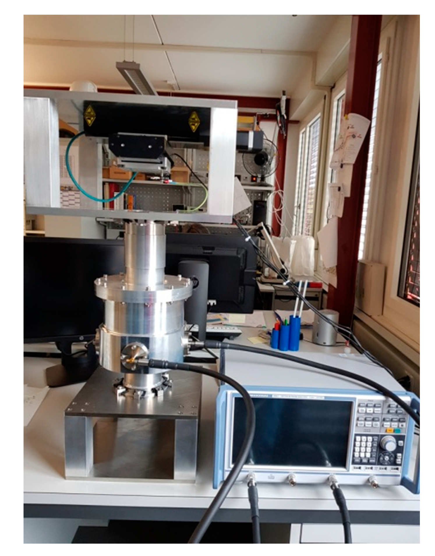
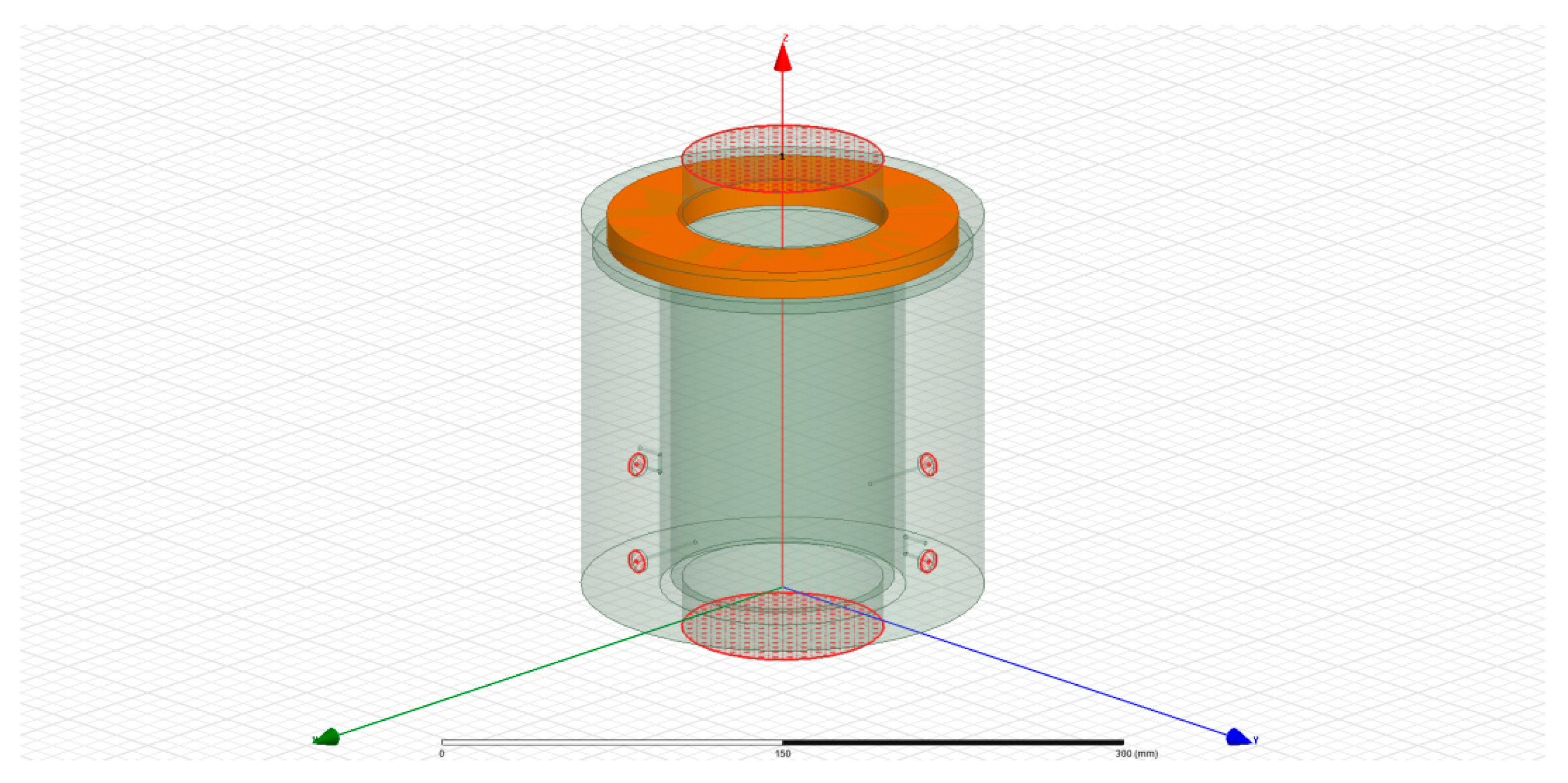
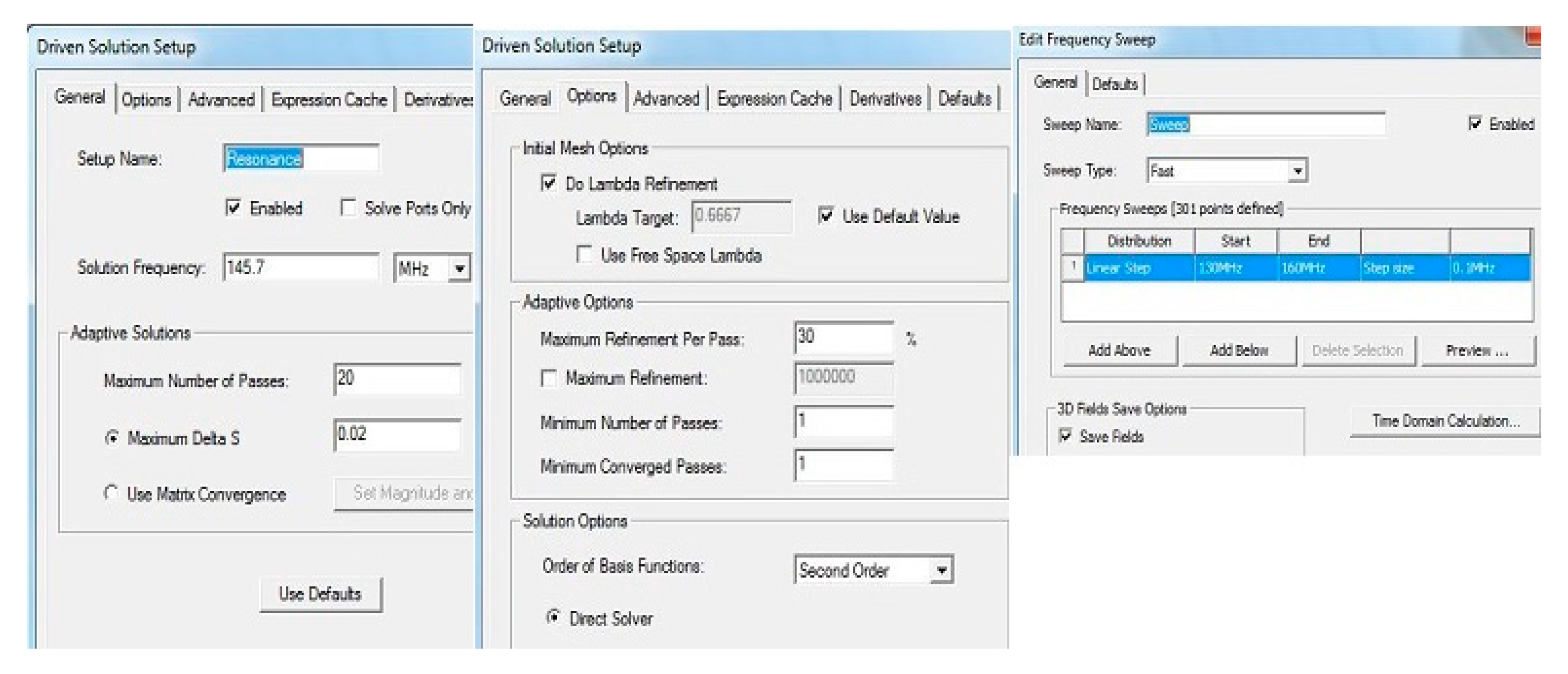
The prototype is characterized in a standalone test bench as shown in Figure 11 [31].

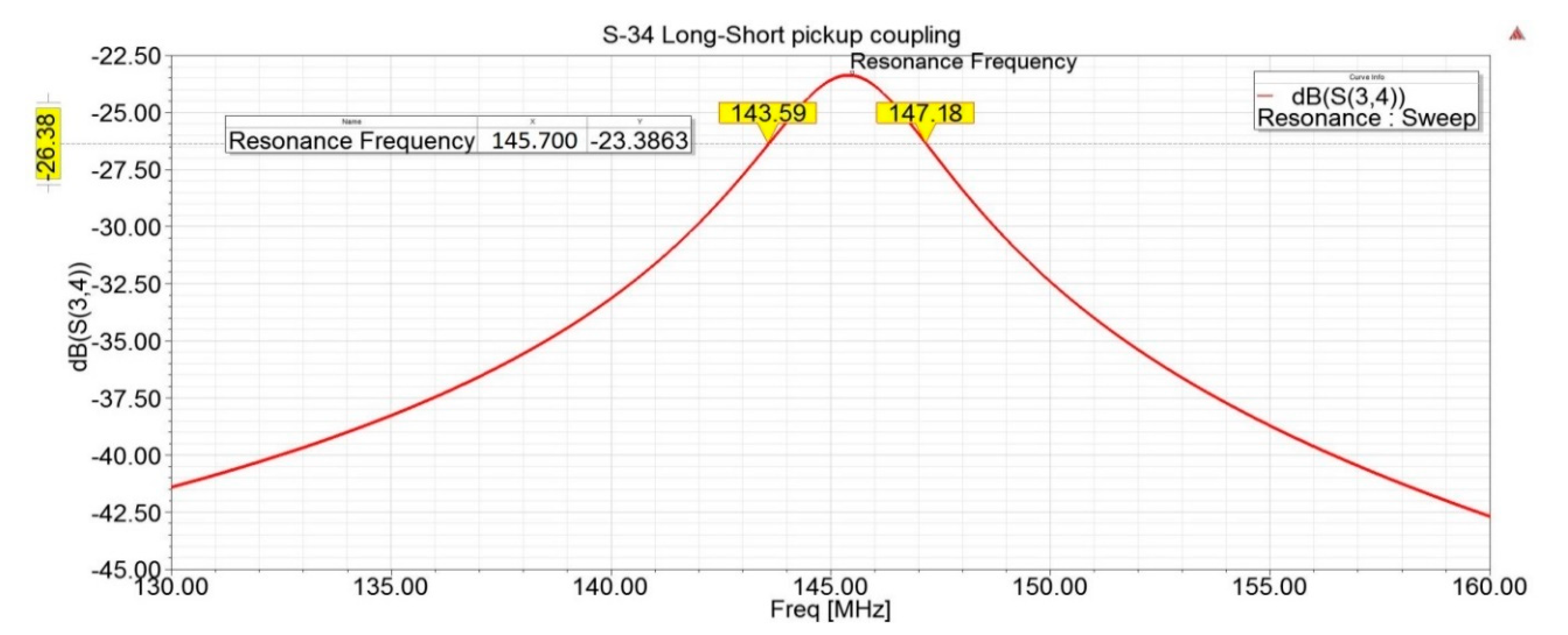
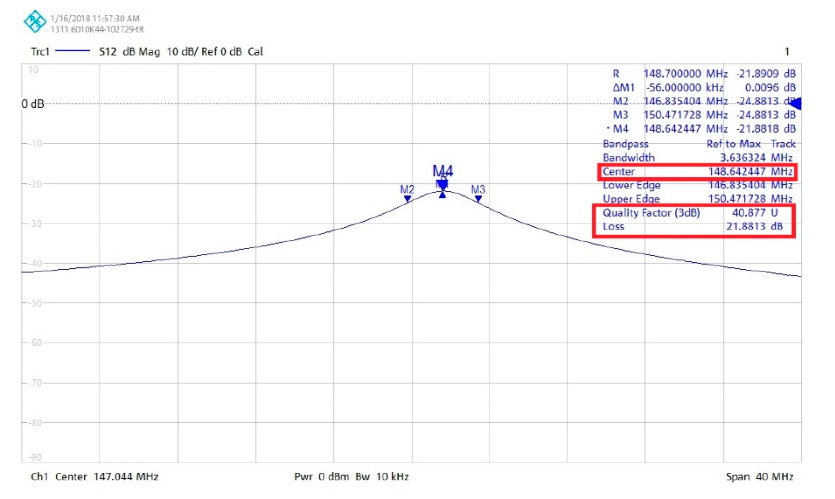
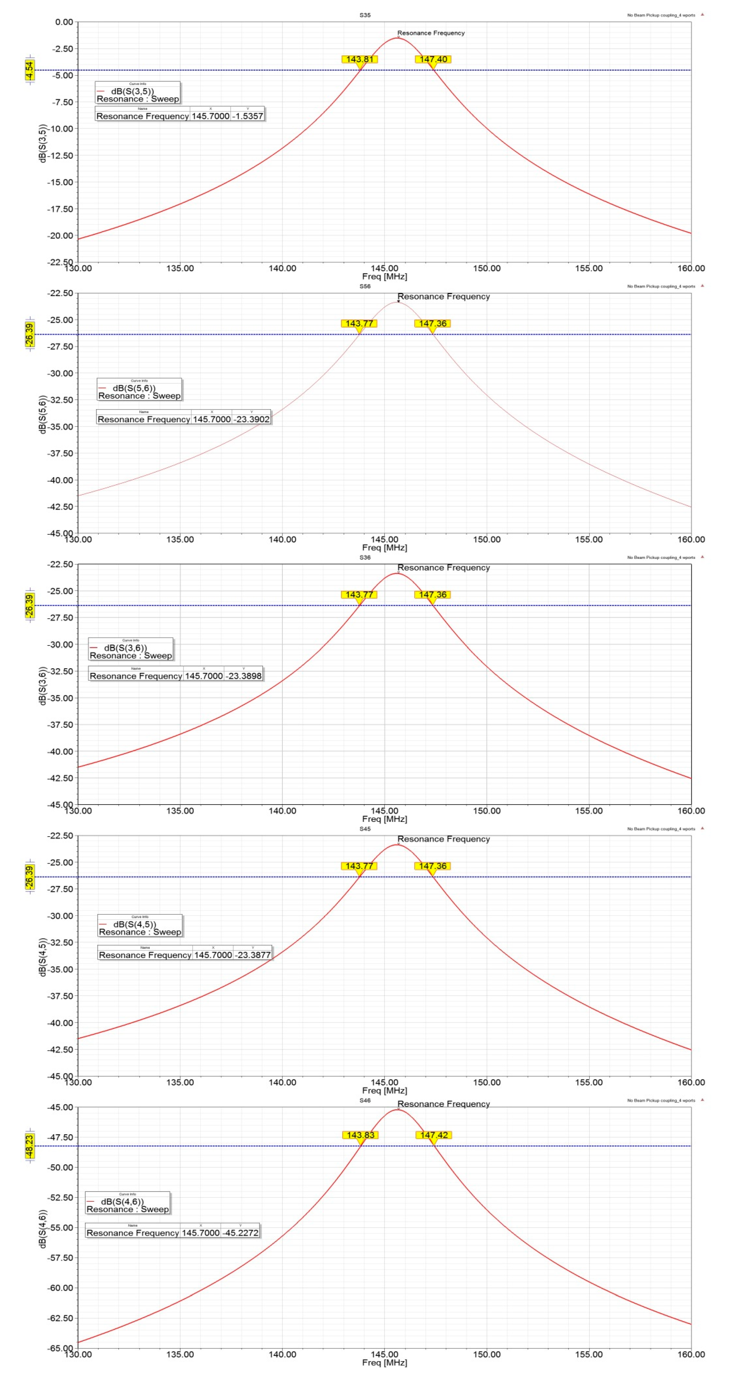
The components of the test bench are: a pair of linear drives from Newport (FCL100) configured as XY; Rhode & Schwarz ZNB8 network analyzer and the device under test (DUT), i.e., the resonator prototype. To characterize the reentrant cavity resonator, network analysis measurement was performed in the absence of a beam analogon. S34, the S-coupling between a long pickup (port 3) and a small pickup (port 4) is shown in Figure 12.

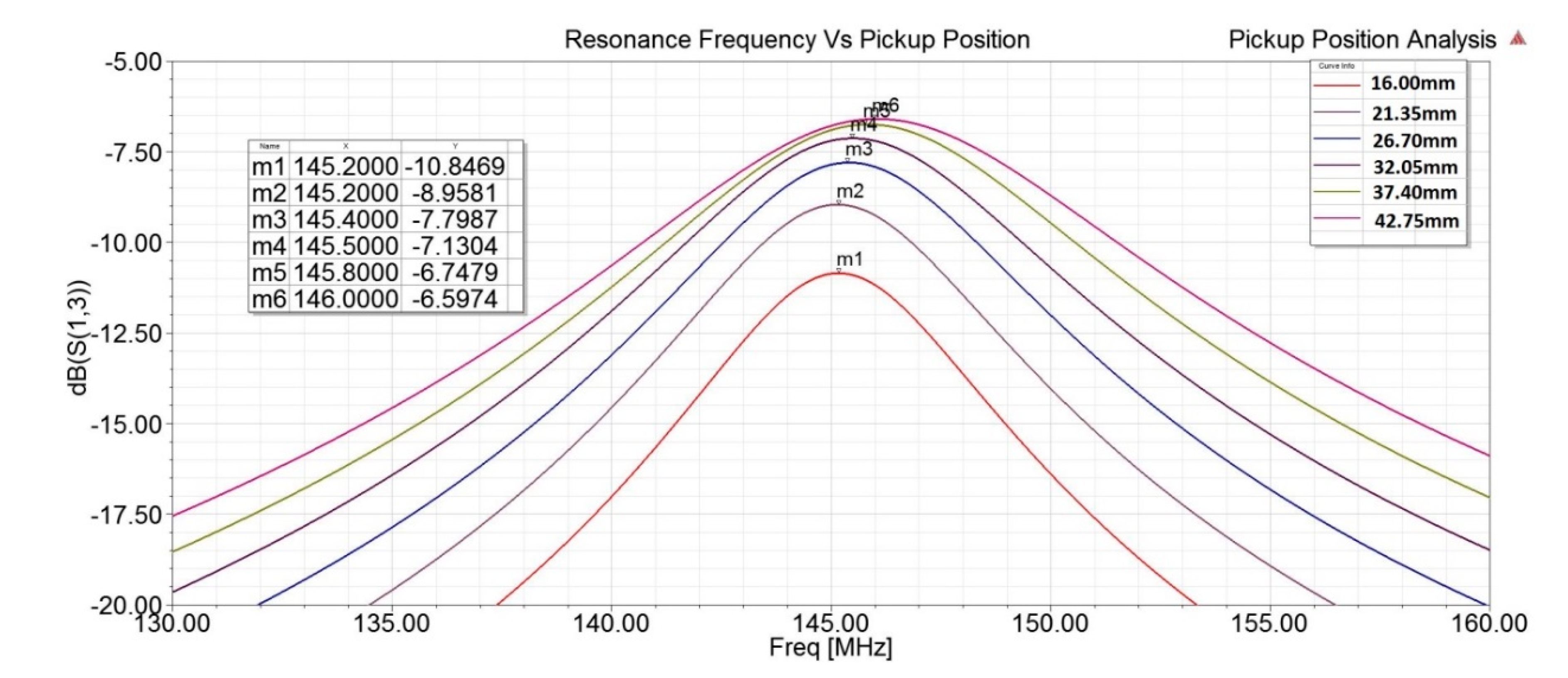
Table 3 summarizes the measured S-coupling parameter between all pickup combinations, resonance frequency and Q factor.

The measurement is done in the absence of a stretched wire to analyze the performance of the stand-alone resonator. The resonance frequency is the peak frequency and the Q factor represents the performance of the resonator. As described in Section 2, the Q factor is a measure of both internal and external losses that is associated with the resonator. This takes into account the lossy dielectrics, imperfect conducting cavity walls, radiated electromagnetic field or external coupling. The 50 Ω external loads that were connected to the pickups represent the main losses and explain the relatively low Q values. S-peak values are slightly larger than those calculated with ANSYS. One reason for this may be the difference between simulated and actual small pickup loops as the measured S-coupling associated with any small pickup loop is different from the simulated S-coupling, with the only exception, the large pickup combination (S-35) being very close to the expected value. Variations in the resonance frequency, S-peak and Q-factor measured values are indicative of the mechanical precision that can be obtained with our prototype and experimental set-up. From the measurements, it could be confirmed that the prototype worked as expected and was in good agreement with the simulation results.

5. Discussion

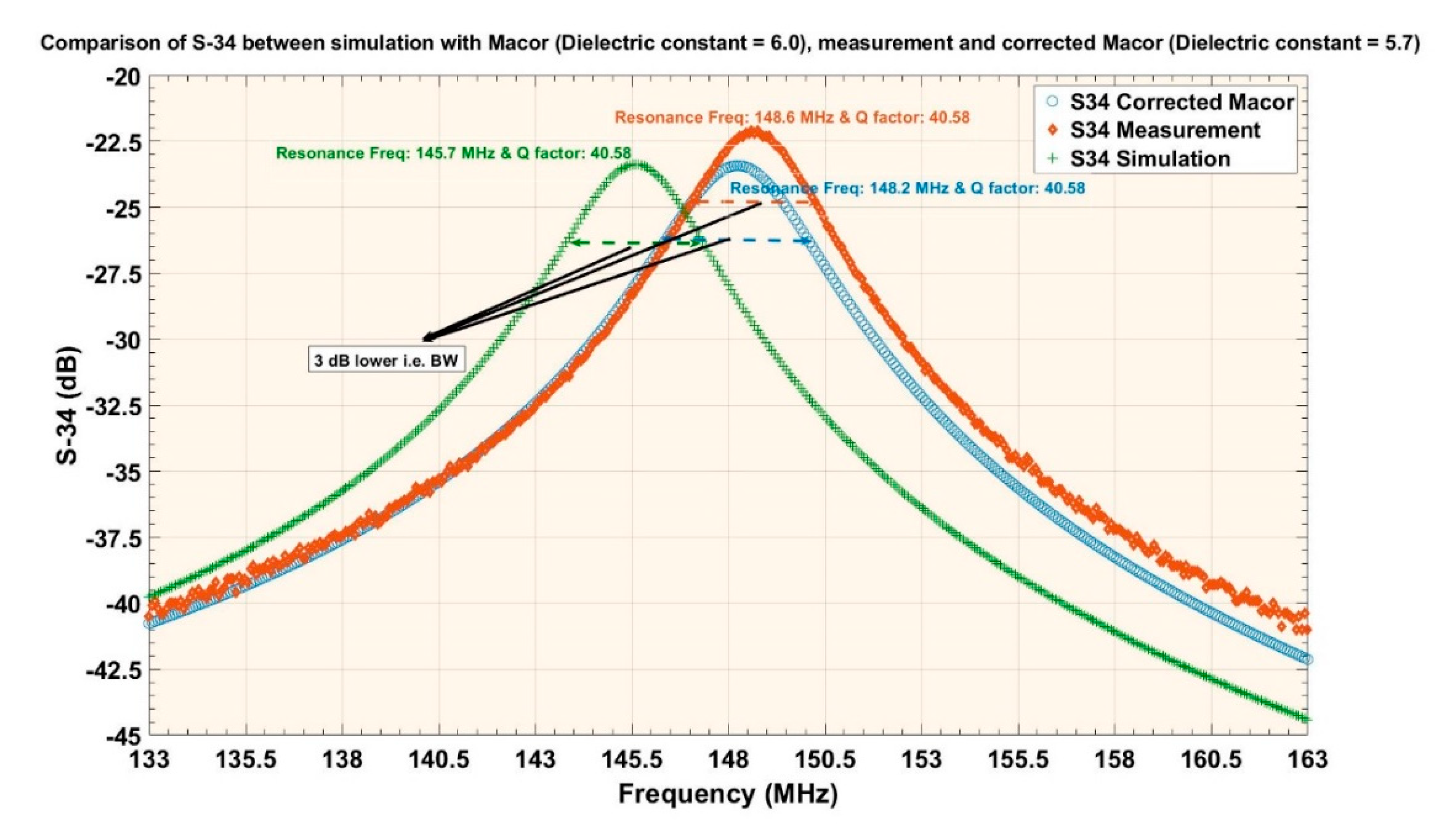
The comparison between the simulation and measurement of S-34 between a long and a small pickup is summarized in Figure 13 and Table 3. The measured Q value is in good agreement with the simulated value. However, the measured resonance frequency is approximately 2% higher than the simulated (design) resonance frequency.

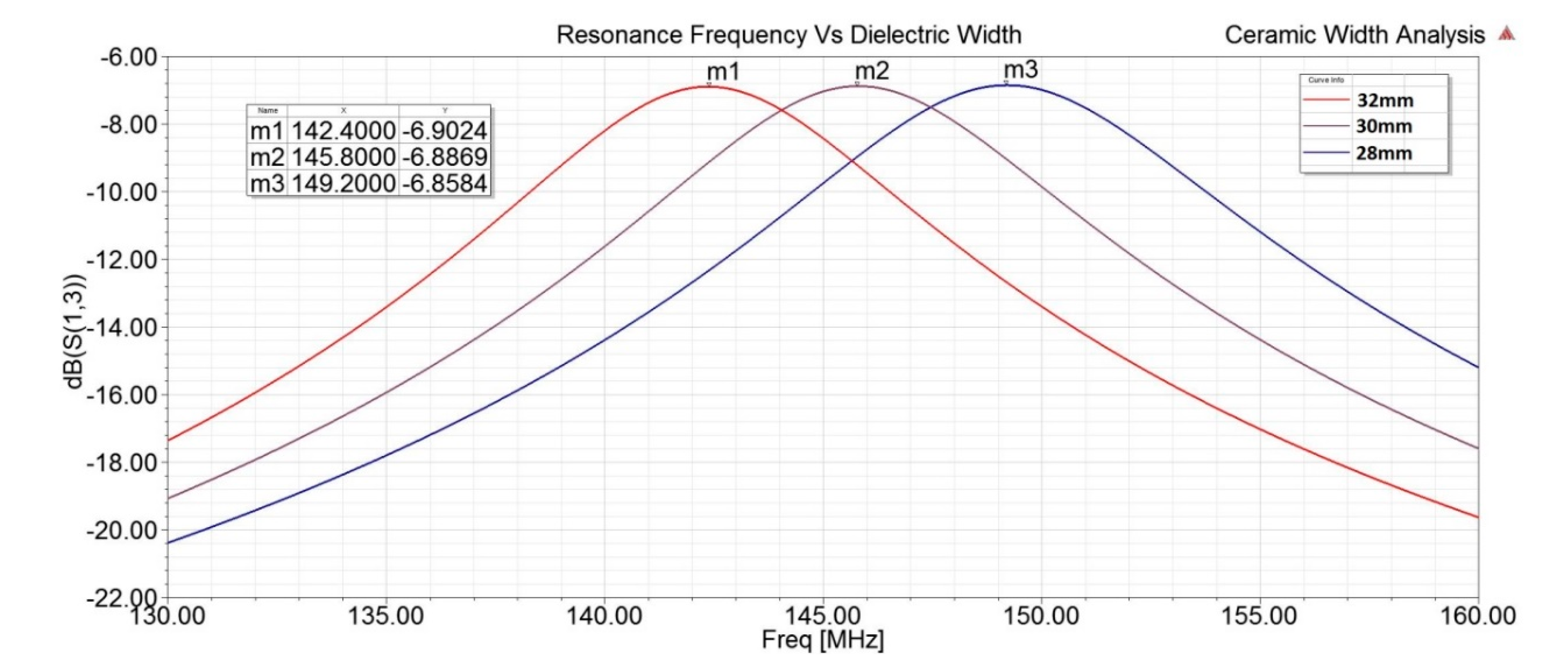
This discrepancy is attributed to the assumption that the Macor ceramic dielectric constant is frequency dependent. In the simulation, the Macor ceramic was assigned a dielectric constant of 6.0 whereas from the measurement, it is evaluated as 5.7, which corresponds to higher frequency of operation. By changing the dielectric constant to 5.7 in the simulation, the simulated resonance frequency matched the measured resonance frequency within a few hundreds of kHz tolerance, as shown in Figure 13. As a consequence, the Macor ceramic’s dimension had to be changed to match the desired resonance frequency of 145.7 MHz. With the help of HFSS simulation, a new Macor ceramic ring of 33 mm width with the same thickness was manufactured and it will be placed in the prototype before testing it on the beamline for final characterization.

Since the test bench results confirmed the HFSS simulations, the expected sensitivity of the system can also be calculated with good confidence. For a given power excitation, the current across the beam entrance and the induced voltage on the pickups can be calculated. For a pickup terminated with an impedance of 50 Ω, the pickup voltage is summarized in

Table 4. Expected pickup voltage for second harmonic component of the beam current. The beam current is denoted in brackets.

2nd Harmonic Beam Component (Beam Current), nA	Pickup Amplitude (nV)	Power Ratio (dBm)
1 (4)	61	−131
0.4 (1.6)	24	−139
0.25 (1)	15	−143

.

This corresponds to the 2nd beam harmonic at 145.7 MHz. For a beam bunch repetition rate of 72.85 MHz, with a pulse length of 2 ns, the frequency spectrum could be calculated using Equation (13). For the second harmonic, the amplitude is approximately 25% of the beam current. Hence, for a beam current of 1 nA, the current at the second harmonic is about 0.25 nA, the pickup amplitude is approximately 15nV (Table 4) and the power ratio is −143 dBm. To read such low signals from the resonator would demand for amplification and high-end ADCs. Assuming a noise contribution of 4dB from the measurement chain, and a signal integration time of 1 second, the expected noise floor is −170 dBm (−174 + 4 dBm), i.e., 0.7 nV. Therefore, the signal-to-noise ratio (SNR) for the prototype can be expected to be around 27.

Since the resonator will be placed beyond the degrader, calibration is important since this is based on its location. Since the velocity spectrum is not monochromatic, some particles in the bunch will be slightly faster and others will be slower than the average bunch velocity. As a consequence, the proton bunch length will increase along the beam line. This is especially true for lower proton beam energy (70 MeV), at which the degrader produces a higher energy spread compared to non-degraded beam. The power spectrum will vary accordingly, affecting the 2nd harmonic amplitude. The second harmonic amplitude is then decreased as Δ increases, i.e., the bunch length is stretched as in Equation (13). This consequently reduces the sensitivity of the reentrant cavity resonator. Due to this dependence of the resonator response, its location should be chosen at a short distance from the degrader.

6. Conclusions

A reentrant cavity resonator was built to measure low proton beam currents in a non-interceptive way. Its design was achieved using the ANSYS simulation tool and the resonance frequency was tuned to match the second harmonic of the beam pulse repetition rate of 72.85 MHz; also, the position of the pickups in the resonator was optimized.

A stand-alone test bench was used to characterize the resonator according to network analysis measurements, which yielded S-parameter coupling between the different pickups. The Q factor is in good agreement with the simulated value. It could be observed that the measured resonance frequency was approximately 2% higher than the simulated (design) resonance frequency, which can be explained by the complex permittivity of the Macor in the resonator.

We conclude that our reentrant cavity resonator is a promising candidate for measuring low proton beam currents in a non-destructive manner. The resonator could replace interceptive monitors, such as ionization chambers to mitigate the associated problems. Moreover, the device can be constructed easily with high precision due to its simple design and radial symmetry. Hence, after mechanical modifications of the PSI PROSCAN beam lines, the reentrant cavity resonator will be validated for ongoing use within the beam line.

References

1. Koziol, H. Beam Diagnostics for Accelerators; CERN Report; CERN Accelerator School: Loutraki, Greece, 2000; pp. 1–44. [Google Scholar] [CrossRef]
2. Wieszczycka, W.; Scharf, W.H. Proton Radiotherapy Accelerators; World Scientific: Singapore, 2001. [Google Scholar]
3. Schippers, J.M.; Dölling, R.; Duppich, J.; Goitein, G.; Jermann, M.; Mezger, A.; Pedroni, E.; Reist, H.W.; Vrankovic, V. The SC cyclotron and beam lines of PSI’s new protontherapy facility PROSCAN. Nucl. Instrum. Methods Phys. Res. B 2007, 261, 773–776. [Google Scholar] [CrossRef]
4. Schippers, J.M. Personal Communication. 2018. [Google Scholar]
5. Dölling, R. Profile, Current, and Halo Monitors of the PROSCAN Beam Lines. AIP Conf. Proc. 2004, 732, 244–252. [Google Scholar] [CrossRef]
6. Duperrex, P.A. Latest Diagnostic Electronics Development for the PROSCAN Proton Accelerator. AIP Conf. Proc. 2004, 732, 268–275. [Google Scholar] [CrossRef]
7. Strehl, P. Beam Instrumentation and Diagnostics; Springer: Berlin/Heidelberg, Germany, 2006. [Google Scholar]
8. Dölling, R. Beam Diagnostics for Cyclotrons. In Proceedings of the CYCLOTRONS, Lanzhou, China, 6–10 September 2010; pp. 344–350. [Google Scholar]
9. Dölling, R. Ionisation chambers and secondary emission monitors at the PROSCAN beam lines. AIP Conf. Proc. 2006, 868, 271. [Google Scholar] [CrossRef]
10. Denard, J.C. Beam Current Monitors. In Proceedings of the CERN Accelerator School, Dourdan, France, 28 May–6 June 2008; pp. 141–155. [Google Scholar]
11. Gasior, M.; Jones, R.; Lefevre, T.; Schmickler, H. Introduction to Beam Instrumentation. In Proceedings of the CERN Accelerator School, Trondheim, Norway, 18–29 August 2013; pp. 23–60. [Google Scholar] [CrossRef]
12. Forck, P.; Kowina, P.; Liakin, D. Beam Position Monitors. In Proceedings of the CERN Accelerator School, Dourdan, France, 28 May–6 June 2008; pp. 187–228. [Google Scholar]
13. Fernandes, M.; Welsch, C.P.; Tan, J. A Cryogenic Current Comparator for the Low-Energy Antiproton Facilities At CERN. In Proceedings of the IBIC, Monterey, CA, USA, 14–18 September 2014; ISBN 9783954501762. [Google Scholar]
14. Vodel, W.; Wittenburg, K.; Knaack, K.; Wendt, M.; Neubert, R.; Nietzsche, S. Highly Sensitive Measurements of the Dark Current of Superconducting Cavities for Tesla Using a Squid Based Cryogenic Current Comparator. In Proceedings of the DIPAC, Lyon, France, 6–8 June 2005; pp. 163–165. [Google Scholar]
15. Walston, S.; Boogert, S.; Chung, C.; Fitsos, P.; Frisch, J.; Gronberg, J.; Hayano, H.; Honda, Y.; Kolomensky, Y.; Lyapin, A.; et al. Performance of a high resolution cavity beam position monitor system. Nucl. Instrum. Methods Phys. Res. A 2007, 578, 1–22. [Google Scholar] [CrossRef] [Green Version]
16. Kim, Y.I.; Ainsworth, R.; Aryshev, A.; Boogert, S.T.; Boorman, G.; Frisch, J.; Heo, A.; Honda, Y.; Hwang, W.H.; Huang, J.Y.; et al. Cavity beam position monitor system for the Accelerator Test Facility 2. Phys. Rev. Spec. Top. Accel. Beams 2012, 15, 042801. [Google Scholar] [CrossRef] [Green Version]
17. Simon, C.; Luong, M.; Chel, S.; Napoly, O.; Novo, J.; Roudier, D.; Rouviere, N.; Baboi, N.; Mildner, N.; Nölle, D. Performance of a reentrant cavity beam position monitor. Phys. Rev. Spec. Top. Accel. Beams 2008, 11, 082802. [Google Scholar] [CrossRef]
18. Luo, Q.; Sun, B.G.; Zhou, Z.R.; Jia, Q.K. Design and Cold Test of Re-Entrant Cavity Bpm for Hls. In Proceedings of the 2011 Particle Accelerator Conference, New York, NY, USA, 28 March–1 April 2011; pp. 420–422. [Google Scholar]
19. Lorenz, R. Cavity beam position monitors. AIP Conf. Proc. 1998, 451, 53–73. [Google Scholar]
20. Sargsyan, V. Comparison of Stripline and Cavity Beam Position Monitors; TESLA Report 2004-03; DESY: Zeuthen, Germany, 2004. [Google Scholar]
21. Feynman, R. Cavity Resonators. In The Feynman Lectures on PHYSICS Vol. 2: Electromagnetism; Addison-Wesley: Boston, MA, USA, 2014; pp. 23.1–23.17. [Google Scholar]
22. Young, P.H. Electronic Communication Techniques; Second Int. Merill: Columbus, OH, USA, 1991. [Google Scholar]
23. Microwave Phase Modulators for Smoothing by Spectral Dispersion. LLE Rev. 1996, 68, 192–208.
24. Collin, R.E. Foundations for Microwave Engineering; Wiley-Interscience: New York, NY, USA, 2001. [Google Scholar]
25. Montgomery, C.G.; Purcell, E.M.; Dicke, R.H. Principles of Microwave Circuits; Dover Publications: Mineola, NY, USA, 1965. [Google Scholar]
26. Kajfez, D. Q Factor; Vector Fields: Oxford, UK, 1994. [Google Scholar]
27. Coulon, F.D. Théorie Et Traitement Des Signaux; Editions Georgi: Laussane, Switzerland, 1984. [Google Scholar]
28. Ansys HFSS Capabilities: High Frequency Electromagnetic Solvers. Available online: https://www.ansys.com/products/electronics/ansys-hfss/hfss-capabilities#cap7 (accessed on 17 September 2018).
29. High Frequency Structure Simulator User’s Guide; ANSOFT Corportation: Pittsburgh, PA, USA, 2005.
30. Macor Technical Data Sheet. Corning Incorportaed. Lighting and Materails. Available online: http://psec.uchicago.edu/ceramics/MACOR%20Data%20Sheet.pdf (accessed on 7 November 2018).
31. Srinivasan, S.; Duperrex, P.A. Reentrant Cavity Resonator for Low Intensities Proton Beam Measurements. In Proceedings of the IPAC2018, Vancouver, BC, Canada, 29 April–4 May 2018; pp. 2341–2344. [Google Scholar]
Figure 1. The fields of the monopole mode i.e., the fundamental mode when the beam points out of the page. The amplitude of the monopole mode is proportional to the bunch charge [15]. (a) is the field configuration in a pill-box cavity, and (b) is the field configuration in a reentrant cavity where the induced E and B field vectors are separated.
Instruments 02 00024 g001
Figure 2. Inspired by Feynman as LC resonator. Lines of E and B are focused separately in the capacitive and inductive zones.
Instruments 02 00024 g002
Figure 3. Universal tuning curve to determine the reentrant cavity resonator length normalized to the free-space wavelength of the microwave frequency in the resonator [23].
Instruments 02 00024 g003
Figure 4. Frequency spectrum of a 2ns pulse train with a repetition rate of 72.85 MHz.
Instruments 02 00024 g004
Figure 5. Dielectric-filled reentrant cavity resonator as beam current monitor. The pickups in the figure represent the large magnetic loops in one plane (as port 3 and 5). Two small magnetic loops are in the other plane (as port 4 and 6). Port 1 is the beam entrance and Port 2 is the beam exit.
Instruments 02 00024 g005
Figure 6. Simulation results for the resonance frequency as a function of the pickup position. Markers represent the resonance frequency and signal coupling to beam entry port for different pickup positions.
Instruments 02 00024 g006
Figure 7. Simulation results for the resonance frequency as a function of the ceramic width. Markers represent the resonance frequency and the signal coupling to beam entry port for different pickup positions.
Instruments 02 00024 g007
Figure 8. Tuning of the resonance frequency by changing the dielectric thickness of the Macor ceramic. Markers represent the resonance frequency and signal coupling to beam entry port for different pickup positions.
Instruments 02 00024 g008
Figure 9. S-34, that is, the coupling between a long pickup and a small pickup. The resonator is tuned to 145.7 MHz (design criteria) and the simulated loaded Q is 40.58.
Instruments 02 00024 g009
Figure 10. Induced E field (a) and H field (b) distribution inside the resonator. Maximum induced E is in the same plane as maximum E of the beam. Similarly, maximum induced B (i.e., H) is in the same plane as maximum B of the beam.
Instruments 02 00024 g010
Figure 11. Stand-alone test bench with the working components: FCL100 series linear drives and a ZNB8 vector network analyzer from Rohde-Schwarz.
Instruments 02 00024 g011
Figure 12. Measured S-34, that is, the cross-talk between a long and a small pickup. Obtained values (marked) at the resonance frequency are the quality factor (Q factor) and the S-coupling.
Instruments 02 00024 g012
Figure 13. Comparison between first simulation ( ε r = 6.0), measurement and simulation with corrected Macor ( ε r = 5.7) of the resonator. Mentioned are The Q factors and the resonance frequency are also mentioned.
Instruments 02 00024 g013