1. Introduction and Motivation
Nonlinearities in RF and microwave systems can take many forms. Historically, nonlinearities are found in circuit elements such as diodes, transistors, amplifiers, mixers, and others. In addition, nonlinearities have been found in other circuit components and are generated by different mechanisms. One of the less common nonlinear mechanisms is passive intermodulation (PIM) distortion, which occurs in antennas [
1,
2], cables, connectors [
2,
3,
4], metal-to-metal junctions [
5,
6], and various components [
7,
8]. A recent development has led to the exploitation of nonlinearities in electronic circuits to detect and track nonlinear targets [
9,
10,
11,
12,
13,
14,
15].
Circuit elements exhibit nonlinear properties either by design or by consequence. By design, P-N junctions, such as diodes, are inherently nonlinear, and this property is exploited for their use in frequency mixers, which are used to upconvert or downconvert signals from one frequency to another. The operation of mixing two signals together to create a new frequency is a nonlinear operation. By consequence, many RF and microwave circuit elements exhibit unintended nonlinear properties. An example is the RF amplifier. Amplifiers are intended to operate linearly, boosting the input signal without creating extraneous frequencies at the output. In practice, creating a linear amplifier is not possible and additional frequency content is generated that distorts the desired signal. Much research has been done to linearize amplifiers [
16,
17,
18,
19,
20]. The unintended frequency content generated by the nonlinear properties of the amplifier interferes with other radar and communication systems [
21,
22,
23], as well as affect the sensitivity of the receiver.
There are other nonlinear effects that are subtler and do not manifest as often. Among these is PIM, which is observed when high power signals interact with components that are weakly nonlinear. Such components do not exhibit measurable nonlinear distortion under normal conditions. In communication systems, the PIM produced can fall close to the fundamental band and interfere with adjacent communication channels [
24,
25]. To combat this, much research has gone into linearizing communication systems [
3,
24,
26]. For close-in intermodulation distortion (IMD), the frequency separation between the fundamental signal and PIM is too small to effectively filter out. Additionally, the communication channels change frequency quickly to accommodate multiple users. So, adaptable filters with large Q values would be needed; however, reconfigurable, high Q filters do not exist. For this reason, adaptive techniques are used to predict and cancel the nonlinearities. Such techniques include predistortion, feedforward linearization, channel equalization, etc. [
27,
28,
29,
30,
31,
32].
Measuring weakly nonlinear RF circuit components requires specialized RF hardware [
3], which itself must be highly linear and devoid of any self-generated nonlinearities. If the measurement system is not highly linear, the measurements will reflect the distortions caused by the test hardware in addition to the device under test (DUT).
Commercially-available high dynamic range PIM measurement systems are accessible today [
33,
34]. These systems are typically designed for specific frequencies, usually around the cell band. They use a two-tone test setup and achieve up to 170 dBc of dynamic range using high Q filters that are fixed in frequency, but lack frequency agility. A commercially-available nonlinear vector network analyzer, PNA-X, demonstrates far more flexibility than the fixed frequency PIM testing systems, and has the ability to vary tone spacings and tone amplitudes [
35]. The PNA-X system also tracks intermodulation (IM) products and harmonics, keeping track of all the nonlinear terms [
36]. However, it lacks the dynamic range necessary to measure nonlinear distortion from weakly nonlinear devices, as they are specified to generate harmonics lower than 60 dBc [
37].
Feedforward cancellation systems have been developed that enable close-in PIM to be measured with a 160-dBc dynamic range, measured from the probe signal power to the spurious free IM frequency [
16,
38,
39,
40]. The systems achieve a large dynamic range by taking great care to linearize their measurement system, which requires high levels of isolation between nonlinear circuit elements in the test setup to the DUTs. These systems also employ an adaptable cancellation system that removes the probe signals before PIM measurements are made. The linearization, isolation, and removal of the probe signal are essential to any high dynamic range measurement system. The downside to constructing such a test setup is the complexity of the system. These systems require iterative feedback from the receiver to cancel the fundamental probe signal. They also require an optimization algorithm to maximize the cancellation of the probe signal to maximize the dynamic range of the measurements.
This paper describes an alternate approach to measuring low level nonlinear distortion from weakly nonlinear targets. The measurement system uses the second harmonic to characterize the nonlinearities of passive RF circuit elements. The measurement system achieves the high dynamic range, of the order of 175 dBc, necessary to measure weakly nonlinear devices while covering a 20% bandwidth, something the PNA-X and other commercially-available systems cannot accomplish. The measurement system is also low complexity, not requiring complicated feedforward cancellation circuits.
Section 1 introduces the mathematics required to characterize nonlinearities from circuit elements.
Section 2 describes basic harmonic measurement techniques to linearize standard RF instrumentation.
Section 3 considers issues in creating a high dynamic range harmonic measurement system.
Section 4 discusses the high dynamic range harmonic measurement system constructed that achieves 175 dBc of dynamic range.
Section 5 presents the results obtained from the measurement system of various RF system components.
Section 6 concludes the paper.
2. Nonlinear Device Modeling and Characterization
To accomplish the goal of characterizing nonlinearities generated by RF circuit components, a nonlinear system model is needed. The model must characterize the nonlinear properties of the devices and predict the behavior of the devices under different conditions. Having the ability to predict the nonlinear response of weakly nonlinear devices enables a system designer to better predict how much distortion will be present in the system. Therefore, the input-output relationship for nonlinear devices needs to be defined.
In general, nonlinear systems do not satisfy the linearity property, i.e., superposition and scaling properties. The output of nonlinear systems contains signals that cannot be represented as a linear combination of the input signals. These signals can be at different frequencies than the input frequencies. In this paper, nonlinear systems are modeled using the power series [
7,
8,
41,
42,
43], which is represented as
where
is the input signal,
is the output signal, and
is the scale factor coefficient of the
nth order nonlinearity.
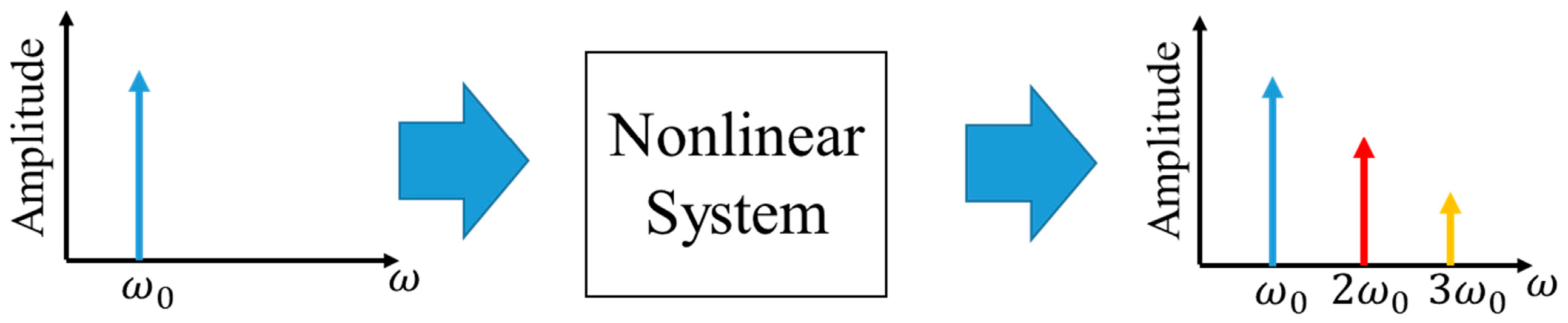
When the input to a nonlinear system is a single frequency, the output consists of harmonics of that frequency occurring at integer multiples of the fundamental frequency. With a single frequency input to the power series given by
, the output can be shown to be [
44]
The amplitude of the frequency domain representations of Equation (2) is illustrated graphically in
Figure 1. Generally, the output amplitude drops as the harmonic order
increases.
Equation (2) expresses the nonlinear system input-output relationship in terms of voltage. Engineers typically prefer to use power units; therefore, the voltage expression is converted to power. The average power of a sinusoidal signal is given by
, where
is the peak voltage and
is the system characteristic impedance. Thus, the power in the harmonics can be represented in a decibel (dB) scale as:
where
is the output power at the
nth harmonic,
is the input power at the fundamental frequency (
),
is a coefficient expressed in dBm
(1−n), and dBm represents power expressed in decibels relative to one milliwatt.
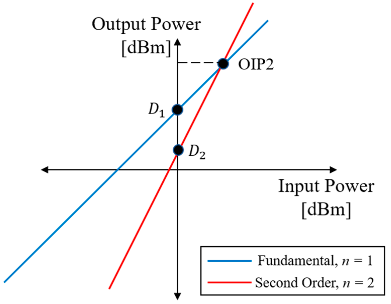
The implications of Equation (3) are that the output-to-input power ratio for the
nth harmonic follows an
relationship in a dB scale. Therefore, a 1-dB increase in the input creates a 2- and 3-dB increase in output power for the second and third harmonics, respectively. In general, the
values are frequency-dependent and characterize the
nth order nonlinear properties of a device. A more commonly found characterization of a device’s nonlinear properties is its output intersect point
, which is the intersection point at which the 1:1 slope of the linear response intersects the
slope of the
nth order nonlinearity. This is shown in
Figure 2 for the second harmonic, i.e.,
.
The relationship between
and
can be found by manipulating Equation (3) to yield:
3. Issues in Creating a High Dynamic Range Harmonic Measurement System
To measure harmonics generated by devices that are not traditionally nonlinear, a high dynamic range (DR) measurement system must be developed. The measurement system must create a highly linear probe signal and must have the ability to measure very weak nonlinear signals in the presence of the large fundamental probe signal.
There are two important aspects of designing a high DR harmonic measurement system: (1) the use of a high DR receiver to measure the weak nonlinear signals in the presence of the high power probe signal; and (2) generation of a highly linear probe single used to probe a DUT. Both the receiver and probe single generator have their unique problems that must be addressed to generate high fidelity, linearized signals. This section addresses these problems.
3.1. Creating a Highly Linear Harmonic Receiver
The first problem in creating a highly linear harmonic receiver is that the measurement hardware is itself nonlinear. The RF front end of a spectrum analyzer consists of nonlinear devices such as amplifiers and mixers. For the results presented in this paper, a National Instruments (NI) (Austin, TX, USA) PXIe-5668R spectrum analyzer is used. The 5668R is specified to generate a second harmonic >69 dBc down from the fundamental, between 700 to 1000 MHz with 0-dBm input power [
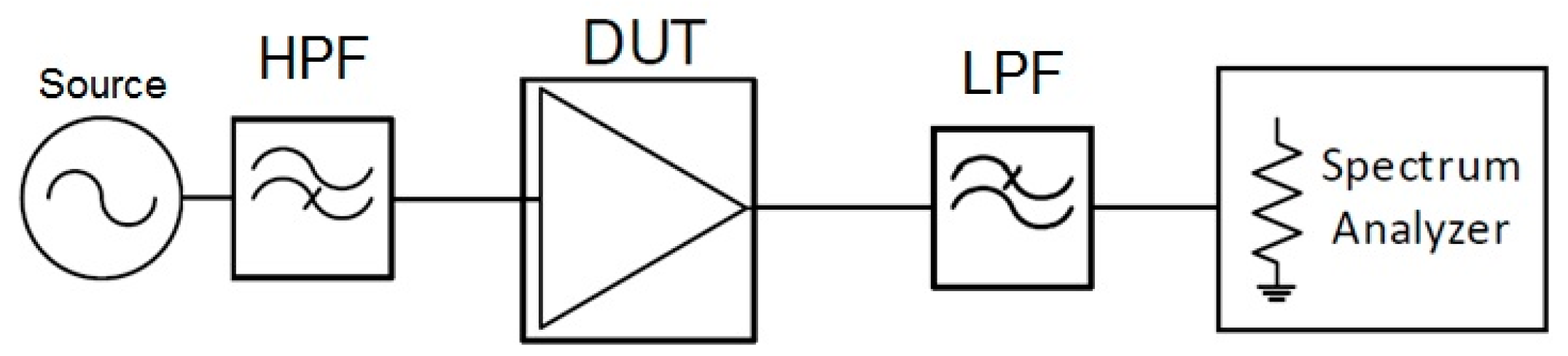
45]. Although the data sheet specifies >69 dBc, the measured self-generated second harmonic is 80 dBc. This 80 dBc of dynamic range is sufficient to make harmonic measurements of strongly nonlinear devices, such as amplifiers, mixers, and diodes, but is inadequate to make measurements of weakly nonlinear elements. The first example of this shown in
Figure 3, which depicts an ideal probe signal entering an amplifier. In
Figure 3, “DUT” stands for “device under test”, “HPF” stands for “high-pass filter”, and “LPF” stands for “low-pass filter”. The DUT is a Mini-Circuits amplifier ZX60-3018G-S+. The fundamental and harmonic responses are made on the PXIe-5668R spectrum analyzer. The choice of filters is very important in architecting a reliable harmonic measurements system [
46].
Three different low-pass filter options are tested using the setup in
Figure 3. These include: (1) no filter; (2) a Mini-Circuits reflective filter VLF-1200; and (3) a Mini-Circuits diplexer RPB-272. When no filter is used, the dynamic range of the test setup is set by the spectrum analyzer, namely 80 dBc. The dynamic range of test setup is increased by filtering out the fundamental frequency before it enters the spectrum analyzer. For every 1-dB attenuation of the fundamental, the self-generated second harmonic of the spectrum analyzer decreases 2 dB. This follows from the relationship in Equation (3). A commercial off-the-shelf (COTS) Mini-Circuits high-pass filter VHF-1200 would be a natural choice, but most COTS filters attenuate the stop band frequencies by creating an impedance mismatch. The result of the mismatch is that the undesired frequencies are reflected and not passed through the filter. The impact of this is examined later. To attenuate the fundamental frequency and to reduce the reflection back into the DUT, a diplexer is used. The low frequency port is terminated in 50 Ω. For this setup, the probe signal is set to 800 MHz and the probe signal power is calibrated to be −20 dBm at the input to the amplifier.
The resolution bandwidth (RBW) on the spectrum analyzer was set to 800 Hz and the internal attenuator was set to 30 dB. The results in
Table 1 illustrate the following two concepts: (1) the spectrum analyzer has the dynamic range to measure the second harmonic response from the Mini-Circuits amplifiers; and (2) the reflective filter alters the test setup and yields false results. If the input power to the spectrum analyzer is 0 dBm, the spectrum analyzer will generate a second harmonic on the order of −90 dBm. Therefore, the reading of −36.3 dBm is well above the self-generation level of the setup and it is a valid reading.
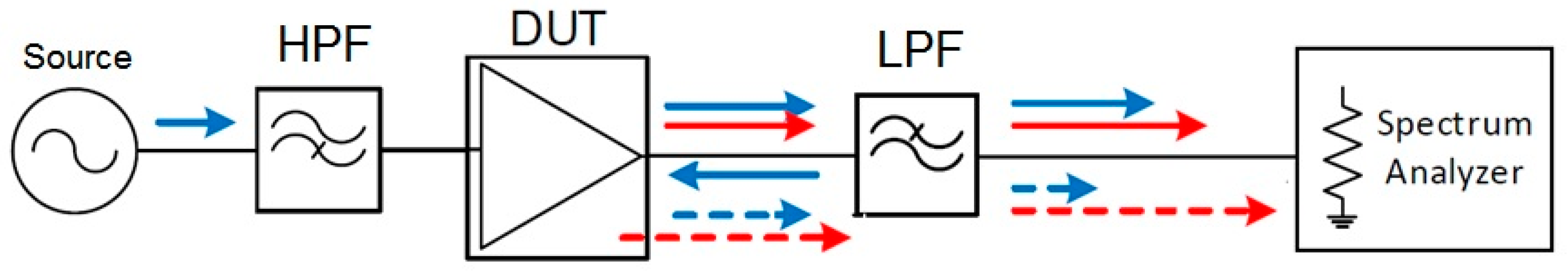
To measure lower level harmonics, the dynamic range of the system needs to be increased. This can be done by using a filter. When a reflective filter is used, the undesired probe signal is reflected causing a reverse traveling wave that enters the output port of the DUT. Once the probe signal enters the output port of the DUT, the probe signal generates additional nonlinearities. The results in
Table 1 show more than a 7-dB increase in the measured second harmonic when the reflective filter is used.
Figure 4 illustrates this reflection and additional generation of the second harmonic when a reflective filter is used.
In
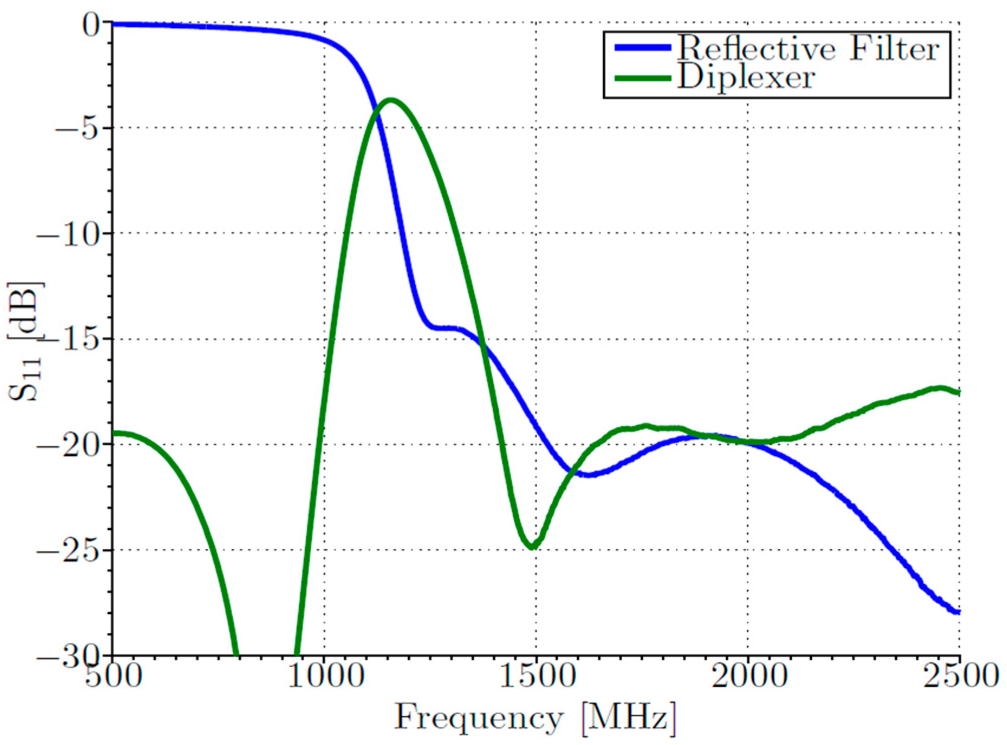
Figure 4, the blue lines represent the probe signal at fundamental frequency, the red lines represent the second harmonic signal, and the dashed lines represent the signals that are generated by the reflected probe signal. For the measurements taken in
Table 1, the setup was calibrated to remove the cable loss and the loss through the filter at the second harmonic. The VHF-1200 and RBF-272 were chosen to have similar losses at 800 and 1600 MHz, the fundamental frequency of the probe signal and its second harmonic under test, respectively. The return loss (
) for both the VHF-1200 and RBF-272 are shown in
Figure 5.
Although the high-pass filter is not needed for this amplifier example, filtering is needed to increase the dynamic range to greater than 160 dBc, the dynamic range needed to measure nonlinearities from passive circuit components. The amount of attenuation needed to achieve a desired dynamic range of
with a current dynamic range of
is given by:
where
is the attenuation needed by the high pass filter at the fundamental frequency. The expression is given in a dB scale. An extra 10 dB is added to the desired dynamic range to ensure that the self-generated nonlinearities are at least a factor of 10 less than the desired minimum detectable nonlinearity. Equation (5) also predicts that the dynamic range is increased by 2 dB for every 1 dB of attenuation in the high-pass filter.
This section has demonstrated the importance of properly linearizing the receive section of a harmonic measurement system. In this section, it was assumed that the probe signal was ideal, i.e., it contained no measurable second harmonic. The next section shows how to ensure proper linearization of the probe signal and illustrates a potential issue when constructing the measurement setup.
3.2. Creating a Harmonic Free Probe Signal
In the previous section, it was assumed that the probe signal was ideal, i.e., it contained no second harmonic. This is not physically possible and this section demonstrates how to create a probe signal that is “ideal enough” to measure weakly nonlinear targets. In the previous section, the fundamental frequency needed to be attenuated in the receiver to measure the second harmonic accurately. In this section, the second harmonic must be removed from the probe to ensure that the measured harmonic is coming solely from the DUT and not the probe signal. If the second harmonic is not adequately attenuated from the probe signal, the measurement system generates a false, self-created second harmonic. This problem is viewed as co-site interference.
3.2.1. Filter Considerations
The amount of second harmonic present in probe signal can never reach zero, or −∞ dB. Therefore, it can only be attenuated to the noise floor of the measurement setup. As in
Section 3.1, the linearity of the measurement system can be increased by filtering. The NI PXI-5651 signal generator used is specified to produce less than 25 dBc of second harmonic when the output power is 0 dBm [
47]. We assumed this value does not change too much when the output power is increased to +10 dBm. With +10 dBm of output power, the 5651 signal generator will produce less than −15 dBm of second harmonic, thereby providing 25 dBc of dynamic range. Thus, if this generator is used without any filtering, accurate second harmonic measurements are made to −5 dBm, including the 10-dB safety factor for signal-to-interference ratio, which is not very useful when trying to make sensitive harmonic measurements. To increase the dynamic range of the receiver, a low-pass filter is used. For the probe signal, the improvement in dynamic range is a 1:1 ratio. So, if the signal generator provides a 25-dBc dynamic range and 160 dBc is desired, the attenuation required for the low pass filter is 145 dB. The general expression for the attenuation needed by the low pass filter is:
where
is the attenuation required of the low-pass filter at the second harmonic and
is the dynamic range of the signal generator. Again, a 10-dB safety factor is built in to ensure 10 dB of signal-to-interference ratio.
Most COTS filters do not provide greater than 100 dB of attenuation required to linearize the probe signal. Therefore, multiple filters need to be cascaded to achieve the large attenuation required. As stated in
Section 3.1, most COTS filters are reflective, and attenuation is achieved in the stop band by an impedance mismatch causing the stop band frequencies to reflect backwards and not pass through it. This reflective nature of filters causes problems.
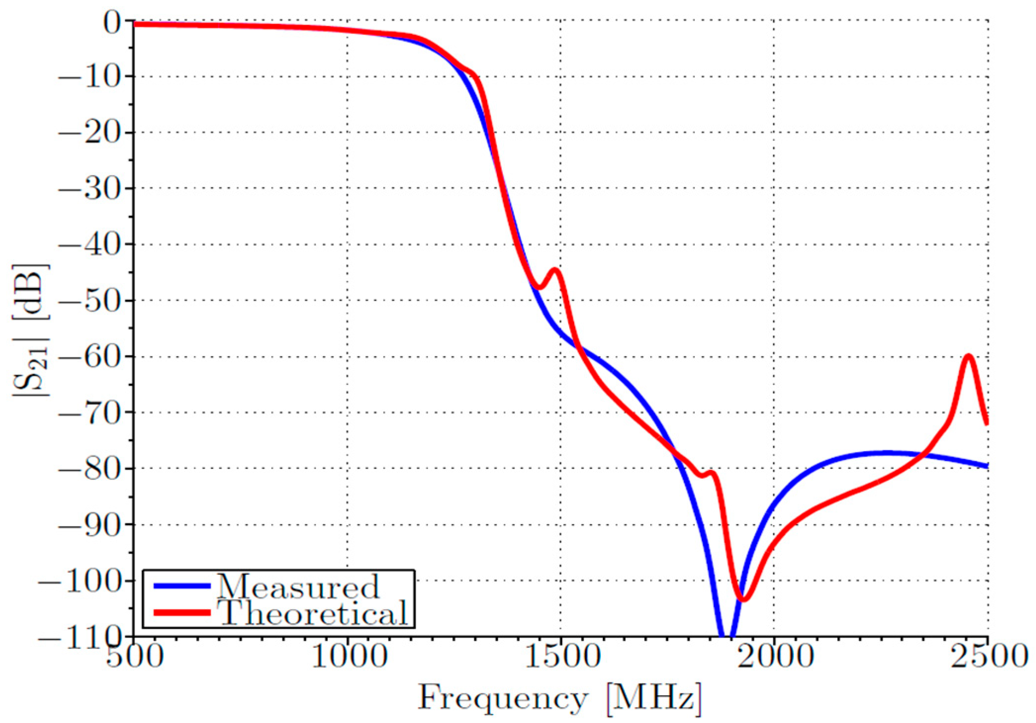
The Mini-Circuits low-pass filter, Model # VLF-1200, has a cut off frequency of 1 GHz. However, the stop band of this filter does not meet the >100-dB attenuation requirement. Therefore, multiple filters need to be cascaded to increase the stop band attenuation.
Figure 6 shows the measured and theoretical
response when two VLF-1200 filters are cascaded. The theoretical cascaded
response was computed as a product of the individual
responses.
When the two reflective low-pass filters are cascaded, the measured and theoretical responses do not closely match. This point is further investigated in [
48], where three reflective low pass filters are cascaded. The measured results when three low-pass filters are cascaded show more discrepancy when compared to the theoretical response.
Using a number of cascaded reflective filters causes large variations in the measurement system’s dynamic range as a function of frequency. If the measurement system operates at a single frequency, a null in the cascaded frequency response can be used. If measurements are taken over a bandwidth of frequencies, the fluctuations in the frequency response would not permit reliable, repeatable, and accurate measurements.
3.2.2. Diplexer Considerations
This leads us to the choice of microwave diplexers for accomplishing the filtering operation. Diplexers are three-port devices which separate power entering a common input into two frequency bands; or conversely, they combine two frequency bands arriving separately into a common output [
49]. Diplexers in which there are adequate guard bands between channels may be designed by suitably connecting two separate, doubly-terminated filters onto a T-junction. These devices are typically employed to connect the transmit and receive filters of a transceiver to a single antenna through a suitable three-port junction [
50,
51]. Diplexers are designed to have low PIM and, therefore, will have low harmonic distortion. With that said, they will generate their own harmonics, but these will be very low, on the order of high-quality cables and connectors, i.e., <−170 dBc. The harmonics generated by the diplexers, cables, and connectors will set a fundamental limit on the dynamic range of the system.
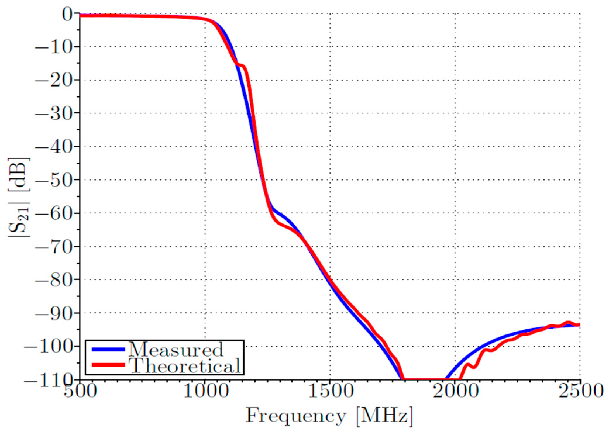
As such, they have the ability to be configured differently for different applications. Diplexers can be used as a low-pass filter by terminating the high frequency port in 50 Ω and using the common port and low frequency port. Unlike reflective filters, diplexers can be cascaded to increase their stop band attenuation. To cascade diplexers in a low-pass configuration, we terminate the high frequency port and connect the common port to the low-pass port of the next diplexer. By connecting the low-frequency port of one diplexer to the common port of another diplexer, the reflections between cascaded diplexers is reduced, when compared to the reflections when reflective filters are cascaded. By terminating the high-frequency port, the stop band frequencies have a path to 50 Ω and the cascaded network is well-behaved.
Figure 7 shows the
response when two diplexers are cascaded in a low-pass configuration.
Figure 7 shows that when two diplexers are cascaded, the measured
closely matches the theoretical response. Comparing
Figure 6 and
Figure 7, we note that cascading diplexers is more desirable than cascading reflective filters for increasing stop band attenuation.
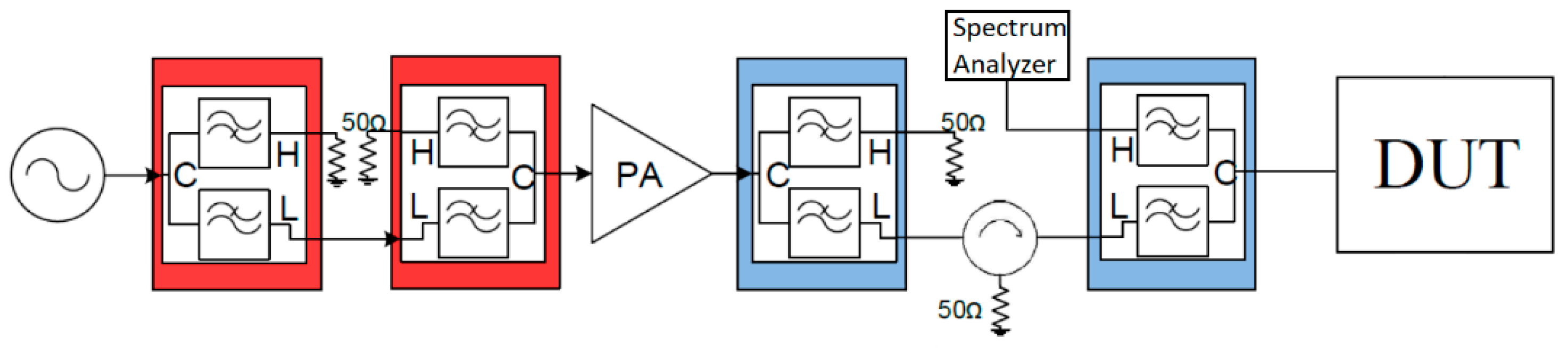
4. System Hardware Design
Using the information from the previous sections, a higher power, high dynamic range harmonic measurement system was constructed. The measurement system was developed to measure second harmonic,
, responses from weakly nonlinear targets. The system also collects data on the linear, fundamental (
) responses from DUTs. The system was designed to measure both the pass through and reflected, linear and second harmonic response. This allows for full characterization of devices. The linear frequency range spans 800 to 1000 MHz and the second harmonic frequency range is 1600 to 2000 MHz. A block diagram of the measurement system is shown in
Figure 8. Note that the second diplexer is flipped to give the harmonics traveling in the reverse direction a path to a 50-Ω termination. Wherever possible, all inputs and outputs are terminated in 50 Ω at both the fundamental frequency and second harmonic.
A NI PXI-5651 signal generator is used to create the probe signal. Next, Mini-Circuits RBF-272 diplexers are used in a low pass configurations to linearize the probe signal, filter out any second harmonic generated by the signal generator. To boost the power of the probe signal, a ZHL-30W-252-S+ Mini-Circuits power amplifier (PA) is used. The probe signal is amplified to 10 W (+40 dBm). The power amplifier is a nonlinear device and generates significant harmonics that need to filtered. Since the fundamental frequency power is at 10 W, high power custom diplexers, manufactured by Reactel, are used.
The high power diplexers are rated up to 100 W continuous wave input power. They are cavity diplexers that provide greater than 80 dB of rejection in the stop band. The passband attenuation is less than 0.4 dB.
Section 3.2 demonstrated the need for a highly linear probe signal; therefore, two such diplexers are cascaded to attenuate the self-generated harmonics below the noise floor. In addition to the diplexers, an isolator is used to isolate the power amplifier output from the DUT and avoid mismatches. The insertion loss of the isolator is 0.2 dB. Thus, the power delivered to the DUT was approximately +39 dBm.
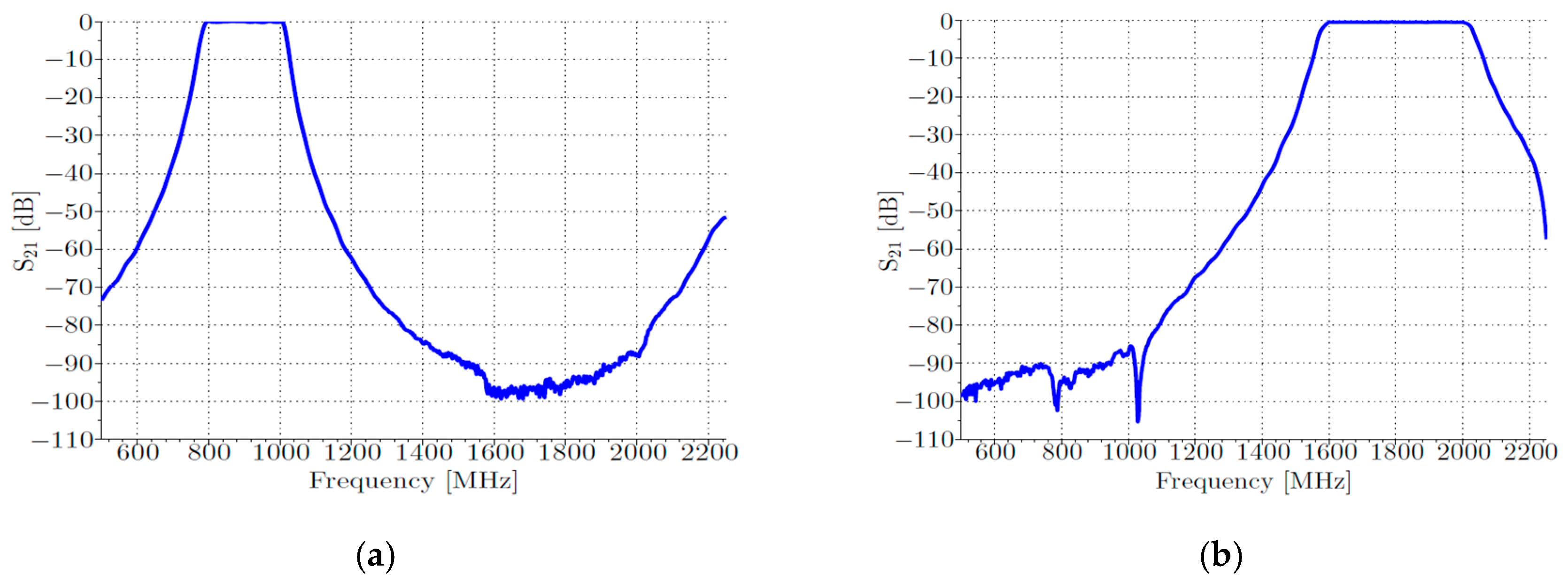
Test results from a single diplexer are presented in
Figure 9. The data in
Figure 9 show the diplexers’ ability to pass the fundamental frequencies, from 800 to 1000 MHz, and attenuate the second harmonics, from 1600 to 2000 MHz.
Figure 9a shows that one cavity diplexer attenuates all harmonics, from 1600 to 2000 MHz, by at least 80 dB with less than 0.4 dB attenuation at the fundamental frequencies, from 800 to 1000 MHz. The high frequency path of the diplexer was also tested and the results are shown in
Figure 9b. Again, the diplexer attenuates the unwanted fundamental frequencies (here it is from 800 to 1000 MHz) by more than 80 dB and it passes the desired harmonic frequencies, 1600 to 2000 MHz, with less than 0.4 dB of loss. Since the diplexers have very little loss in the pass band, they do not absorb a significant amount of pass band energy.
A measured link-budget for a 900-MHz tone, used as the probe signal, is presented in
Table 2. Note from
Table 2 that going from D to E for the second harmonic shows a loss of 113.4 dB. However, according to
Figure 9a, the loss is seen to be around 95 dB. This discrepancy is probably due to the fact that the
measurements are made on a network analyzer and the results in
Figure 9a are likely limited by the network analyzer’s noise floor or the internal coupling.
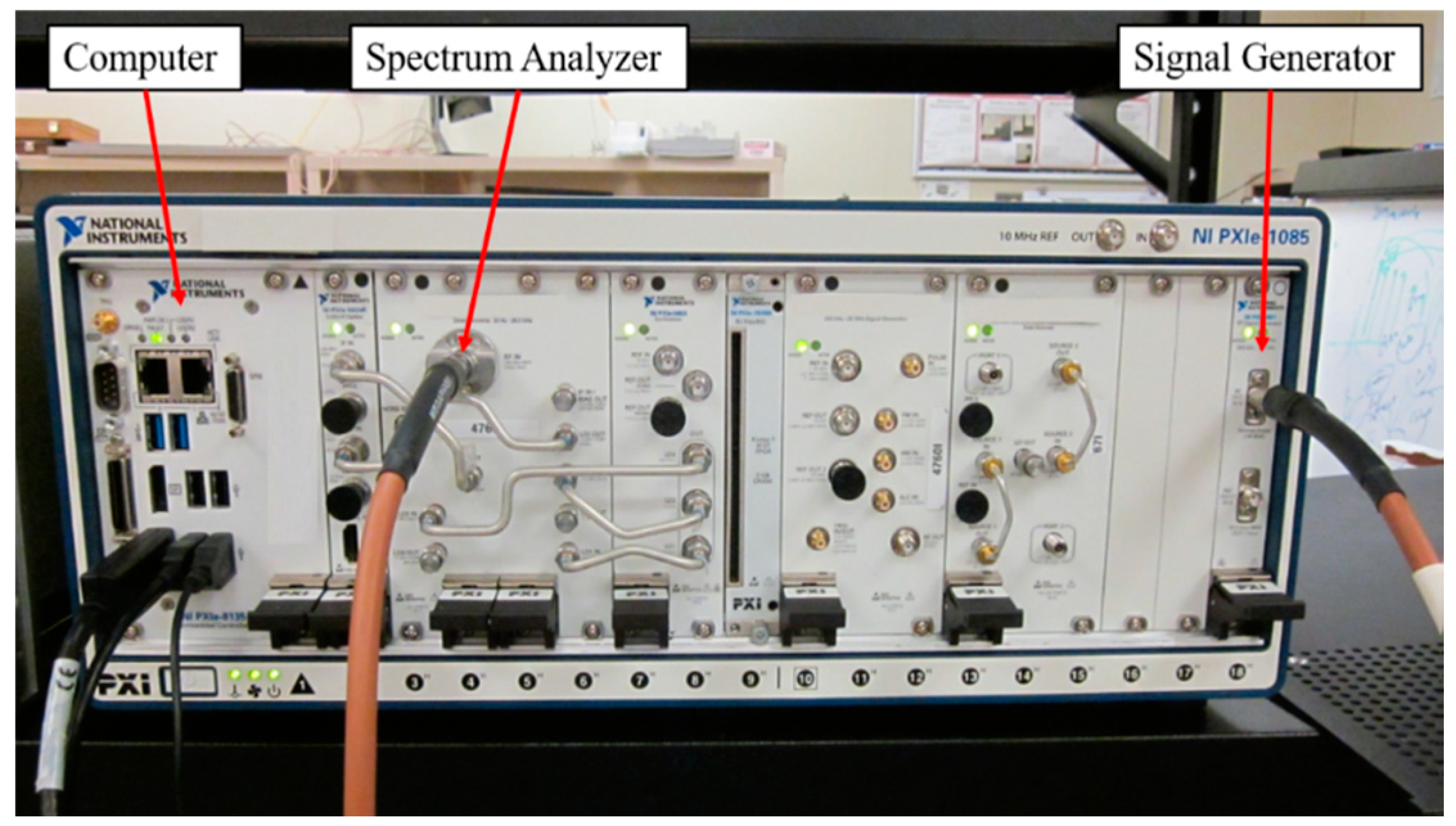
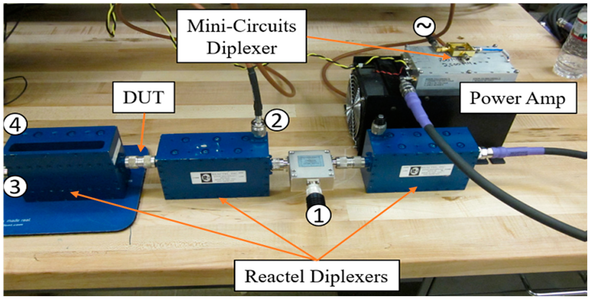
Photographs of the NI chassis and the RF components (Mini-Circuits and Reactel diplexers and power amplifier) are shown in
Figure 10 and
Figure 11, respectively.
The receiver hardware is straightforward. The probe signal, at the fundamental frequency, is separated from the second harmonic using another high power diplexer. The fundamental frequency passing through the DUT is measured at port 3 in
Figure 11. The output second harmonic is measured at port 4. The spectrum analyzer has an 80-dBc dynamic range; coupling this with the 80-dB of loss provided by the Reactel diplexer yields a system dynamic range of over 200-dBc, according to Equation (5). However, the theoretical 200-dBc dynamic range is unachievable, as in practice, the system would be noise limited before 200-dBc can be achieved. The noise floor of the receiver is measured to be less than 135 dBm. With the probe signal measured to be greater than 40 dBm and the noise floor below 135 dBm, the system’s dynamic range is estimated to be greater than 175 dB.
5. System Test Results
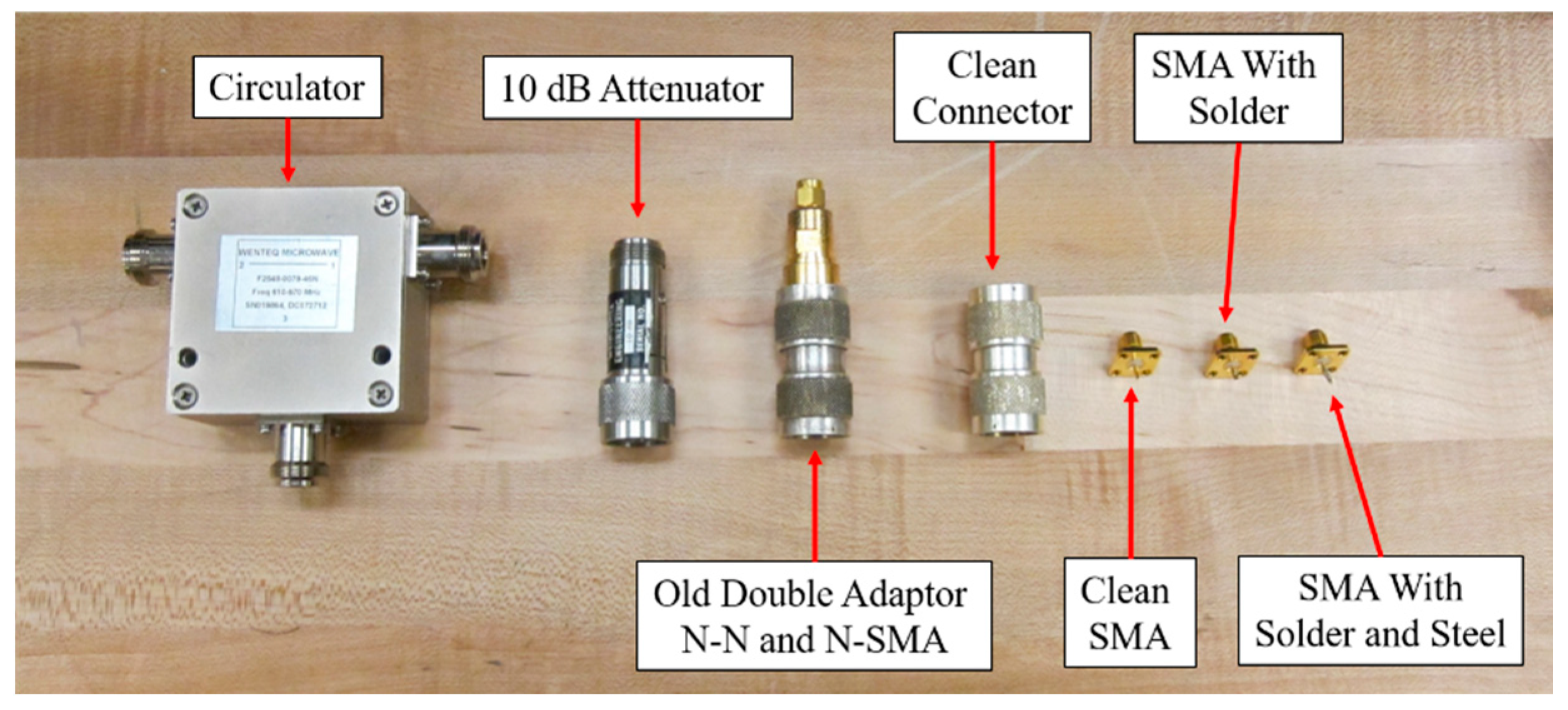
The high dynamic range measurement system described in
Section 4 was used to measure the second harmonic response from a variety of circuit elements. The passive devices tested are shown in
Figure 12.
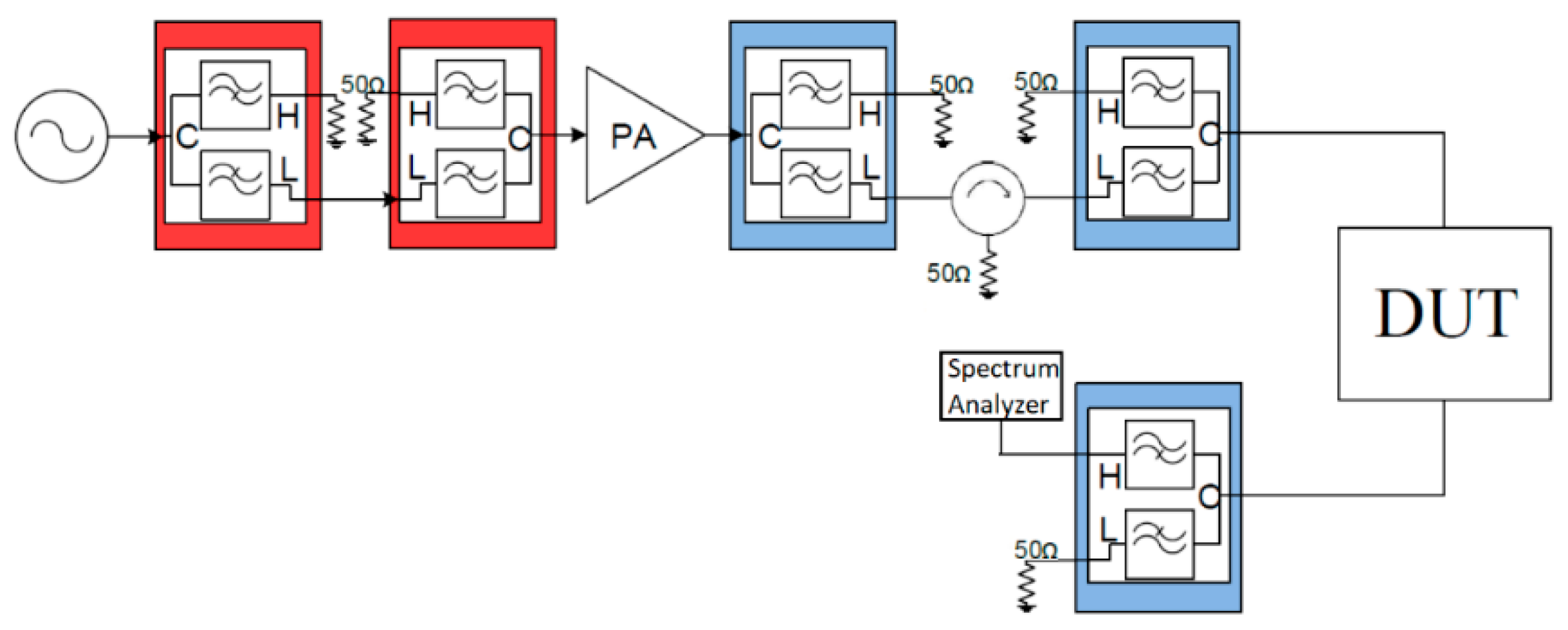
The two port devices were tested for their input and output harmonic generation while the one-port devices could only be tested for their reflected harmonic generation. Test setups for the harmonic through and harmonic reflection measurements are shown in
Figure 13 and
Figure 14, respectively.
Since the spectrum analyzer only has one input port, the fundamental and second harmonic at the output of the DUT need to be measured via two separate measurements. Therefore, the loading conditions of the two measurements are slightly different. The spectrum analyzer is matched to 50 Ω throughout the bands of interest with an input reflection coefficient of less than 20 dB, which provides a 99% power transfer. The differences between the loading conditions for the fundamental and second harmonic measurements is therefore expected to be negligible compared to using a 50 Ω termination. Thus, we believe that any mismatches between the two measurement setups would result in an insignificant difference in nonlinear distortion generated.
The test results are summarized in
Table 3. The values are shown for
in Equation (3), the units for which are dBm
−1. A lower value, i.e., more negative, indicates better harmonic suppression.
The results from the open circuit and new N(m)-N(m) adaptor show the minimum detectable coefficient the setup can measure. The open circuit and new adaptor test cases are the baseline measurements used for monitoring the spurs created at the second harmonic and the noise floor, which determines the system dynamic range. Any significant contributions from the higher-order harmonics to the second harmonic would be indicated in this measurement. The observations from this measurement indicated that distortion created from these higher order harmonics are below the noise floor.
Since a mixer, by design, is a nonlinear component whose nonlinearity is essential for frequency conversion [
52], it shows much higher
values. Attenuators typically consist of resistors connected in T- or Π-configurations with dissimilar metal contacts, which results in
values of about 60 dB higher than the detection floor. The intense RF magnetic field across the ferrite disk excites nonlinear behavior in a circulator [
53], which explains its higher values. The old, i.e., well-used, adaptor shows about 20-dB increase in
compared to the new adaptor, which may be ascribed to possible corrosion caused by wear and tear and environmental effects. Connectors terminated in solder and steel show higher
values compared to the unterminated connector due to the effect of the dissimilar metal contacts, with steel adding about a 20-dB higher value, consistent with the results reported in [
54,
55]. The mixer serves as a reference for traditionally nonlinear devices.
Table 3 shows that the nonlinear response from the mixer is about 90 dB over the circulator, about 120 dB over the attenuator, and about 145–170 dB over the adaptors, at an input of 0 dBm.

 ,
, 


