Abstract
The temperature dependence of the two superconducting gaps in pressurised at 155 GPa with a critical temperature of 203 K has been determined using a data analysis of the experimental curve of the upper critical magnetic field as a function of temperature in the framework of the two-band s-wave Eliashberg theory. Two different phonon-mediated intra-band Cooper pairing channels in a regime of moderate strong couplings have the key role of the pair-exchange interaction between the two gaps, giving the two non-diagonal terms of the coupling tensor, which are missing in the single-band s-wave Eliashberg theory. The results provide a prediction of the different temperature dependence of the small and large gaps as a function of temperature, which provides evidence of multigap superconductivity in .
1. Introduction
The conventional superconducting state of low-critical-temperature superconductors was described in 1957 by BCS theory in the dirty limit where multiple bands are reduced to an effective single band, with a single large isotropic Fermi surface and a large Fermi energy where Cooper pairs are formed by the exchange of a low-energy phonon. In this classical approximation, the critical temperature is controlled by the phonon energy and the electron–phonon interaction. The material-dependent critical temperature is calculated by using the isotropic Eliashberg theory [1,2] with a single electron–phonon spectral function for the average interaction over the Fermi surface. This function in different materials was determined previously from the inversion of tunnelling data, while now it is calculated using density functional theory (DFT). The single-band approximation was also found to break down for the element niobium [3] in 1970, but it was considered at that time a mere curiosity. In the framework of the single-band approximation, the Fermi energy is far from the band edges and therefore, the critical temperature does not show strong anomalous variations as a function of the lattice compressive strain induced by pressure. On the contrary, in the clean limit the multiband metals with different Fermi surfaces give multigap superconductivity where the non-diagonal terms in the coupling tensor are determined by an additional fundamental interaction beyond Cooper pairing in quantum matter: the pair exchange between different gaps. While the hot topic for the majority of the scientific community searching for the mechanism of superconductivity in high- cuprate superconductors was focusing the search for unconventional pairing mechanisms using a single-band approximation, few authors focused on controlling the pair-exchange interaction in the multigap scenario. The Bianconi Perali Valletta (BPV) theory predicted that, by tuning the perovskite lattice strain or charge density, there is an asymmetric dome for the amplification of the critical temperature with a threshold at the Lifshitz transition for the appearance of a new Fermi surface and a maximum at the Lifshitz transition for opening a neck in the appearing Fermi surface. This is driven by the Fano–Feshbach resonance due to configuration interactions between large and small gaps in the BEC-BCS regime and in the BCS regime controlled by the non-diagonal terms of the coupling tensor of multigap superconductivity [4]. Subsequently, in 2001, superconductivity at 40 K in magnesium diboride () was discovered [5], which was described by the two-band Eliashberg theory [6,7] and the BPV theory [8,9]. The very large family of iron-based superconductors discovered in 2008 [10] provided key evidence for a plurality of scenarios of multiband superconductivity, with the number of bands ranging from three to five and the chemical potential tuned near a Fano–Feshbach resonance or shape resonance between superconducting gaps [11]. In the last two decades, the extensive search for the pairing mechanism in cuprates remained focused on strong correlation and d-wave symmetry of the order parameter [12]. The history of high pressure as a tool to find novel high-temperature superconductors begins with studies [13,14] focusing on pressurised metallic hydrogen and pre-compressed hydrides until the prediction of Duan [15] and the experimental discovery [16] in 2015. In 2015, after the discovery, the need for multigap superconductivity theory to describe the 203 K superconductivity in sulfur hydride was noticed [17]. For 8 years, superconductivity in high-pressure hydrides [18] has been thoroughly investigated in the single-band approximation [19,20]. The experimental hints that multiband superconductivity could be relevant were, first, the anomalous pressure-dependent isotope effect [21] and, later, the experimental evidence of the linear trend of the upper critical field () as a function of temperature [22]. In this article, we analyse the experimental data available on as a function of temperature using the multiband Eliashberg theory using the simplest possible model still able to grasp the relevant physics of this system. Since we do not know exactly all the input parameters that the two-band Eliashberg theory needs, we will examine some possible scenarios that will be verified with future experiments. While we were writing this work, Eremets’ group showed tunnelling effect measurements [23] on at a pressure of 155 GPa with a critical temperature of 203 K, which clearly show two superconducting gaps: a small one at 10 meV and a large one at 25 meV at 77 K. Our work was motivated by these new experimental data [23], which clearly demonstrate that this system is multiband. Our very simple model showed that the experimental data can be easily explained in Eliashberg’s two-band s-wave theory and that the electron–phonon coupling is on the order of , i.e., half of what it had previously been valued [22].
2. The Model
We will try to explain the experimental data using the simplest possible model that, despite the approximations, still manages to grasp the fundamental physical aspects. Obviously, by giving up some approximations but losing simplicity, it will be possible to further improve the agreement with the experimental data. The electronic structure of the compound can be approximately described by some large Fermi surfaces and a small appearing Fermi surface [17]. The relevant bands, following the nomenclature present in the literature, have been named [21] with the numbers 8, 9, 10, 11. Band 10 is narrow (about 400 meV) and is associated with the large gap (50 meV), while the other three bands are broad and are associated with the small gap (20 meV). In our model, the density of states of the band indicated with index 2 will correspond to band 10 and thus, its density of states at the Fermi level ( (cell·eV)), while the band indicated with index 1 will correspond to bands 8, 9 and 11 with a density of states at the Fermi level ( (cell·eV)), which corresponds to the sum of the contributions of these three bands. To calculate the gaps and the critical temperature within the two-band Eliashberg equations [24], one has to solve four coupled equations for the gaps and the renormalization functions , where i is a band index (that ranges between 1 and 2) and are the Matsubara frequencies. The imaginary-axis equations [6,24,25,26,27] read:
In these equations we have defined
and and . The parameters and are the scattering rates from non-magnetic and magnetic impurities, while is the Heaviside function and is a cutoff energy. The quantities are the elements of the Coulomb pseudopotential matrix. The electron–phonon coupling constants are defined as . In the more general situation, the solution of Equations (1) and (2) requires a large number of input parameters (four functions and twelve constants). We have to introduce in the equations four electron–phonon spectral functions , four elements of the Coulomb pseudopotential matrix , four nonmagnetic and four paramagnetic impurity-scattering rates. However, some of these parameters can be extracted from experiments and some can be fixed with suitable approximations. In particular, we put because, when the order parameter is in an s-wave, the intraband component of the impurity scattering rate has no influence on superconductive properties (Anderson theorem), while the interband contribution usually has a negligible effect [28]. This parameter () is relevant only for strongly disordered non-s-wave superconductors, but this is not the case. The same can be performed for the scattering rate from magnetic impurities that are absent, so we set . We assume that the shape of the electron–phonon functions is the same and we rescale them by changing the parameter , i.e., we write . The function , normalized to have electron–phonon coupling constant and equal to one, is taken from reference [29] and was calculated for a pressure value very close to the experimental one. The values of interband coupling are not independent because as the interband Coulomb pseudopotential . is the density of states at the Fermi level for band i. We know the values of and , so, in this way, we have six free parameters: three and three . For reducing the number of free parameters, we suppose that the Coulomb pseudopotential is zero. This choice was made solely to reduce the number of free parameters and in any case does not substantially change the physical picture of the system. In this way, we will determine the minimal values of the electron–phonon coupling constant, because if the Coulomb pseudopotential is different from zero the coupling constants will be slightly greater. The Coulomb pseudopotential usually is a relevant parameter just for the fullerenes [30]. At the end we have three free parameters: , and . The strategy is to reproduce exactly (if it is possible) the experimental values of the small gap at K ( meV) [23] and the experimental critical temperature K. In this way, we fix the three free parameters and after, we can calculate other physical observables and compare them with experiments. Finally, we use for obtaining the numerical solution of the Eliashberg equations a cut-off energy meV and a maximum quasiparticle energy meV. We will examine three cases that roughly exhaust all possible cases: the first case with loosely coupled bands, the second case with intermediately coupled bands and the third case with strongly coupled bands. Of course, in all cases examined the calculated critical temperature exactly reproduces the experimental one.
3. Results
In the case of loosely coupled bands, the electron–boson coupling-constant matrix becomes:
to produce a , which represents the average of electron–phonon coupling. In Figure 1, the self energy functions and obtained by solving the Eliashberg equations in the real axis formulation at K are shown, while in the upper and lower insets are shown, respectively, the electron–phonon spectral function and the superconductive density of states, always at K. The value of the small gap at K is equal to meV and becomes equal to 10 meV at K, which is exactly the measured value. The big gap at K is equal to meV and becomes equal to 38.7 meV at K, as is shown in Figure 2, a value greater than the experimental value [23] of 25 meV. In the case where the bands have an intermediate coupling, the electron–boson coupling-constant matrix is:
to produce . Also in this case, the value of the small gap at K is exactly reproduced, while at K, the values of the two gaps are meV and meV, respectively.
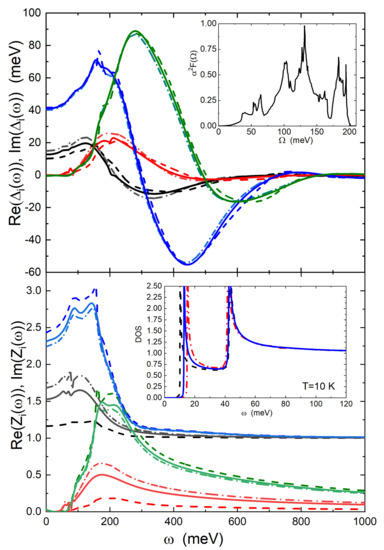
Figure 1.
Real and imaginary parts of the self energy functions and obtained by solving the Eliashberg equations at K in the real axis formulation in the three cases examined (weak band coupling, dashed dotted lines; intermediate band coupling, solid lines; and strong band coupling, dashed lines) are shown as functions of energy in the upper () and lower () panels. In the inset of the upper panel, the electron-phonon spectral function is shown, while in the inset of lower panel, the superconductive densities of states at K are shown (weak case, red dashed dotted line; intermediate case, dark blue solid line; and strong case dashed black line).
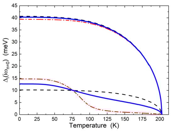
Figure 2.
Calculated temperature dependence of the two gaps is shown (weak case, red dashed dotted line; intermediate case, dark blue solid line; and strong case, dashed black line).
In the case where the bands are strongly coupled, the electron–boson coupling-constant matrix is:
to produce . As in the last case, the value of the small gap at K is exactly reproduced, while at K the values of the two gaps are meV and meV, respectively. In this case, there is very little difference between the small gap values at 10 K and 77 K because the bands are strongly coupled and the temperature behavior is completely different, as it is possible to see in Figure 2. We can observe that in all cases we are in a regime of moderate strong coupling (, and ) less than lead (). Of course, this model is very simple and, for example, to improve the agreement with the experimental data (large gap), one should consider that the density of states around the Fermi level is not constant but would make the model more complicated [31] and add nothing really essential to the physical explanation of the system.
At this point, to decide which of the three cases examined is more plausible, we need to examine other experimental data such as the temperature dependence of the upper critical magnetic field. The multiband Eliashberg model developed above can also be used to explain the experimental temperature dependence of the upper critical magnetic field. The experimental data [22] show that displays a linear dependence on temperature over an extended range, as found in a strong coupling one-band superconductor or in a multiband superconductor. Now we check if our model is able to explain the experimental data. We will calculate the temperature behavior of the upper critical magnetic field in the three cases examined and we will see if these experimental data will allow us to decide which of the three cases best describes this system. For the sake of completeness, we give here the linearized gap equations in the presence of a magnetic field with non-magnetic impurity scattering [32,33]. In the following, is the Fermi velocity of band j and is the upper critical magnetic field:
with . We know that the ratio of the Fermi velocities of the two bands [21] is approximately equal to , so we assume that . In this way, using the previously used electron–phonon coupling constants, we will fix the Fermi velocity relative to band 2 in order to obtain the best fit of the experimental data. We find in the first case (weak coupling between the two bands) = 8.455 × m/s and consequently, 6.504 × m/s. The value of the upper critical magnetic field at a very low temperature is T. We proceed in the same way in the second case, where the bands have an intermediate coupling between them. Now, we find 8.511 × m/s and 6.547 × m/s with T. For the last case, where the bands are strongly coupled, we find × m/s and × m/s with T. Figure 3 shows the theoretical curves relative to the three cases compared with the experimental data [22]. It is clearly seen that in all cases the experimental measurements can be reproduced well. In order to decide which of the three cases best describes the physics of the system, it would be necessary to make tunnelling measurements to determine the trend of the two gaps as a function of the temperature, which, as we can see in Figure 2, is profoundly different in the three cases. Most likely, it is also possible to reproduce the upper critical field as a function of temperature with the one-band Eliashberg theory, but with double the electron–phonon coupling value [22]. We have not produced this calculation solely because the experimental data of tunneling presented by Emerets [23] clearly show two distinct values of the gaps.
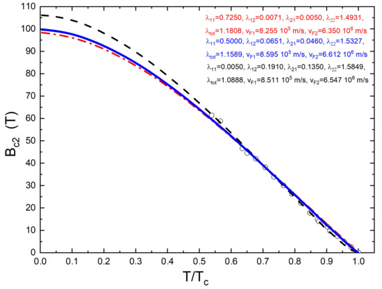
Figure 3.
Experimental temperature dependence of the upper critical field in (open circles) from reference [22] and the theoretical curves (weak case, red dashed dotted line; intermediate case, dark blue solid line; and strong case, dashed black line) obtained by solving the Eliashberg equations for the upper magnetic field with the input parameters of the three cases.
4. Conclusions
We have been able to shed light on the quantum mechanism giving the high critical temperature of pressurised driven by unconventional anisotropic electron–phonon interactions in different portions of multiple Fermi surfaces and pair-exchange interactions, like the Majorana exchange force in nuclear heterogeneous matter made of multiple components [34,35,36] and the coexistence of weak and strong electron–phonon interactions. The critical temperature, the small gap value and the behavior of the upper critical field as a function of temperature are well-reproduced in the framework of two-band s-wave Eliashberg theory with Cooper pairing in a regime of moderate strong coupling and a small essential pair-exchange interaction missing in the standard single-band model. We predict a different temperature dependence of the large and small gaps in the intermediate two-gap regime proposed for pressurized sulfur hydride. To establish which of the three discussed regimes is the correct one, it will be necessary to obtain further experimental data on the temperature dependence of the two gaps by using tunnelling measurements.
Author Contributions
G.A.U. and A.B. contributed equally to conceptualization, methodology, formal analysis, original draft preparation and writing. All authors have read and agreed to the published version of the manuscript.
Funding
This research received no external funding.
Data Availability Statement
Not applicable.
Acknowledgments
G.A. Ummarino acknowledges partial support from the MEPhI.
Conflicts of Interest
The authors declare no conflict of interest.
References
- Carbotte, J.P. Properties of boson-exchange superconductors. Rev. Mod. Phys. 1990, 62, 1027. [Google Scholar] [CrossRef]
- Ummarino, G.A. Eliashberg Theory. In Emergent Phenomena in Correlated Matter; Pavarini, E., Koch, E., Schollwöck, U., Eds.; Forschungszentrum Jülich GmbH and Institute for Advanced Simulations: Jülich, Germany, 2013; pp. 13.1–13.36. [Google Scholar]
- Hafstrom, J.W.; MacVicar, M.L.A. Case for a second energy gap in superconducting niobium. Phys. Rev. B 1970, 2, 4511. [Google Scholar] [CrossRef]
- Bianconi, A.; Valletta, A.; Perali, A.; Saini, N.L. Superconductivity of a striped phase at the atomic limit. Phys. C Supercond. 1998, 296, 269–280. [Google Scholar] [CrossRef]
- Nagamatsu, J.; Nakagawa, N.; Muranaka, T.; Zenitani, Y.; Akimitsu, J. Superconductivity at 39 K in magnesium diboride. Nature 2001, 410, 63–64. [Google Scholar] [CrossRef]
- Ummarino, G.A.; Gonnelli, R.S.; Massidda, S.; Bianconi, A. Two-band Eliashberg equations and the experimental Tc of the diboride Mg1-xAlxB2. Phys. C 2004, 407, 121–127. [Google Scholar] [CrossRef][Green Version]
- Daghero, D.; Calzolari, A.; Ummarino, G.A.; Tortello, M.; Gonnelli, R.S.; Stepanov, V.A.; Tarantini, C.; Manfrinetti, P.; Lehmann, E. Point-contact spectroscopy in neutron-irradiated M11B2. Phys. Rev. B 2006, 74, 174519. [Google Scholar] [CrossRef]
- Innocenti, D.; Caprara, S.; Poccia, N.; Ricci, A.; Valletta, A.; Bianconi, A. Shape resonance for the anisotropic superconducting gaps near a Lifshitz transition: The effect of electron hopping between layers. Supercond. Sci. Technol. 2010, 24, 015012. [Google Scholar] [CrossRef]
- Innocenti, D.; Poccia, N.; Ricci, A.; Valletta, A.; Caprara, S.; Perali, A.; Bianconi, A. Resonant and crossover phenomena in a multiband superconductor: Tuning the chemical potential near a band edge. Phys. Rev. B 2010, 82, 184528. [Google Scholar] [CrossRef]
- Kamihara, Y.; Watanabe, T.; Hirano, M.; Hosono, H. Iron-Based Layered Superconductor La[O1-xFx]FeAs(x=0.05-0.12) with Tc=26 K. J. Am. Chem. Soc. 2008, 130, 3296–3297. [Google Scholar] [CrossRef]
- Bianconi, A. Shape resonances in superstripes. Nat. Phys. 2013, 9, 536–537. [Google Scholar] [CrossRef]
- Gonnelli, R.S.; Calzolari, A.; Daghero, D.; Natale, L.; Ummarino, G.A.; Stepanov, V.A.; Ferretti, M. Evidence for pseudogap and phase-coherence gap separation by Andreev reflection experiments in Au/La2-xSrxCuO4 point-contact junctions. Eur. Phys. J. B 2001, 22, 411–414. [Google Scholar] [CrossRef]
- Ashcroft, N. Metallic hydrogen: A high-temperature superconductor? Phys. Rev. Lett. 1968, 21, 1748. [Google Scholar] [CrossRef]
- Ashcroft, N. Hydrogen dominant metallic alloys: High temperature superconductors? Phys. Rev. Lett. 2004, 92, 187002. [Google Scholar] [CrossRef] [PubMed]
- Duan, D.; Liu, Y.; Tian, F.; Li, D.; Huang, X.; Zhao, Z.; Yu, H.; Liu, B.; Tian, W.; Cui, T. Pressure-induced metallization of dense (H2S)2H2 with high-Tc superconductivity. Sci. Rep. 2014, 4, 6968. [Google Scholar] [CrossRef]
- Drozdov, A.; Eremets, M.; Troyan, I.; Ksenofontov, V.; Shylin, S. Conventional superconductivity at 203 kelvin at high pressures in the sulfur hydride system. Nature 2015, 525, 73–76. [Google Scholar] [CrossRef]
- Bianconi, A.; Jarlborg, T. Lifshitz transitions and zero point lattice fluctuations in sulfur hydride showing near room temperature superconductivity. Nov. Supercond. Mater. 2015, 1, 37. [Google Scholar] [CrossRef]
- Purans, J.; Menushenkov, A.P.; Besedin, S.P.; Ivanov, A.A.; Minkov, V.S.; Pudza, I.; Kuzmin, A.; Klementiev, K.V.; Pascarelli, S.; Mathon, O.; et al. Local electronic structure rearrangements and strong anharmonicity in YH3 under pressures up to 180 GPa. Nat. Commun. 2021, 12, 1765. [Google Scholar] [CrossRef]
- Gorkov, L.P.; Kresin, V.Z. Colloquium: High pressure and road to room temperature superconductivity. Rev. Mod. Phys. 2018, 90, 011001. [Google Scholar] [CrossRef]
- Pickett, W.E. Colloquium: Room temperature superconductivity: The roles of theory and materials design. Rev. Mod. Phys. 2023, 95, 021001. [Google Scholar] [CrossRef]
- Jarlborg, T.; Bianconi, A. Breakdown of the Migdal approximation at Lifshitz transitions with giant zero-point motion in the H3S superconductor. Sci. Rep. 2016, 6, 24816. [Google Scholar] [CrossRef]
- Mozaffari, S.; Sun, D.; Minkov, V.S.; Drozdov, A.P.; Knyazev, D.; Betts, J.B.; Einaga, M.; Shimizu, K.; Eremets, M.I.; Balicas, L.; et al. Superconducting phase diagram of H3S under high magnetic fields. Nat. Commun. 2019, 10, 2522. [Google Scholar] [CrossRef]
- Eremets, M.I. Communication in “Superconductivity in superhydrides. New developments”. In Proceedings of the SUPERSTRIPES 2023 Conference, Ischia, Italy, 25 June–1 July 2023. [Google Scholar]
- Ummarino, G.A.; Tortello, M.; Daghero, D.; Gonnelli, R.S. Three-band s± Eliashberg theory and the superconducting gaps of iron pnictides. Phys. Rev. B 2009, 80, 172503. [Google Scholar] [CrossRef]
- Ghigo, G.; Gozzelino, G.A.U.L.; Tamegai, T. Penetration depth of Ba1-xKxFe2As2 single crystals explained within a multiband Eliashberg s± approach. Phys. Rev. B 2017, 96, 014501. [Google Scholar] [CrossRef]
- Torsello, D.; Ummarino, G.A.; Gozzelino, L.; Tamegai, T.; Ghigo, G. Comprehensive Eliashberg analysis of microwave conductivity and penetration depth of K-, Co-, and P-substituted BaFe2As2. Phys. Rev. B 2019, 99, 134518. [Google Scholar] [CrossRef]
- Ummarino, G.A.; Gonnelli, R.S. Breakdown of Migdal’s theorem and intensity of electron-phonon coupling in high-Tc superconductors. Phys. Rev. B 1997, 56, R14279. [Google Scholar] [CrossRef]
- Daghero, D.; Calzolari, A.; Delaude, D.; Gonnelli, R.S.; Tortello, M.; Ummarino, G.A.; Stepanov, V.A.; Zhigadlo, N.D.; Karpinski, J.; Putti, M. Point-contact study of the role of non-magnetic impurities and disorder in the superconductivity of MgB2. Phys. C 2007, 460–462, 975–976. [Google Scholar] [CrossRef]
- Villa-Cortés, S.; De la Peña-Seaman, O. Effect of van Hove singularity on the isotope effect and critical temperature of H3S hydride superconductor as a function of pressure. J. Phys. Chem. Solids 2022, 161, 110451. [Google Scholar] [CrossRef]
- Cappelluti, E.; Grimaldi, C.; Pietronero, L.; Strassler, S.; Ummarino, G.A. Superconductivity of Rb3C60: Breakdown of the Migdal-Eliashberg theory. Eur. Phys. J. B 2001, 21, 383–391. [Google Scholar] [CrossRef]
- Ummarino, G.A.; Gonnelli, R.S. Possible explanation of electric-field-doped C60 phenomenology in the framework of Eliashberg theory. Phys. Rev. B 2002, 66, 104514. [Google Scholar] [CrossRef]
- Mansor, M.; Carbotte, J.P. Upper critical field in two-band superconductivity. Phys. Rev. B 2005, 72, 024538. [Google Scholar] [CrossRef]
- Ummarino, G.A.; Tortello, M.; Daghero, D.; Gonnelli, R.S. Predictions of multiband s±strong-coupling Eliashberg theory compared to experimental data in iron pnictides. J. Supercond. Nov. Magn. 2011, 24, 247–253. [Google Scholar] [CrossRef]
- Mazziotti, M.V.; Raimondi, R.; Valletta, A.; Campi, G.; Bianconi, A. Spin–orbit coupling controlling the superconducting dome of artificial superlattices of quantum wells. J. Appl. Phys. 2022, 132, 193908. [Google Scholar] [CrossRef]
- Mazziotti, M.V.; Jarlborg, T.; Bianconi, A.; Valletta, Q. Room temperature superconductivity dome at a Fano resonance in superlattices of wires. Europhys. Lett. 2021, 134, 17001. [Google Scholar] [CrossRef]
- Vittorini-Orgeas, A.; Bianconi, A. From Majorana theory of atomic autoionization to Feshbach resonances in high temperature superconductors. J. Supercond. Nov. Magn. 2009, 22, 215–221. [Google Scholar] [CrossRef]


Disclaimer/Publisher’s Note: The statements, opinions and data contained in all publications are solely those of the individual author(s) and contributor(s) and not of MDPI and/or the editor(s). MDPI and/or the editor(s) disclaim responsibility for any injury to people or property resulting from any ideas, methods, instructions or products referred to in the content. |
© 2023 by the authors. Licensee MDPI, Basel, Switzerland. This article is an open access article distributed under the terms and conditions of the Creative Commons Attribution (CC BY) license (https://creativecommons.org/licenses/by/4.0/).