DC Transport and Magnetotransport Properties of the 2D Isotropic Metallic System with the Fermi Surface Reconstructed by the Charge Density Wave

Abstract

We report the ground state stabilization and corresponding electrical transport and magnetotransport properties of a 2D metallic system with an isotropic Fermi surface reconstructed by a charge density wave. The onset of the charge density wave is a spontaneous process, stabilized by the condensation energy gain due to the self-consistent mechanism of topological reconstruction of the Fermi surface and opening of the pseudo-gap around it. We address the signature of the uni-axial reconstruction in terms of the measurable quantities, such as the intra-band transport properties, including the one-particle density of states, the total and effective concentration of electrons, and the Hall coefficient. Additionally, we analyze the magnetotransport properties of the system reconstructed by the bi-axial, checkerboard-like charge density wave, under conditions of magnetic breakdown. It manifests huge quantum oscillations in diagonal components of magnetoconductivity, while the Hall conductivity changes sign, varying the external magnetic field with a finite region of vanishing Hall coefficient in between.

1. Introduction

Charge density waves (CDWs) have been present in solid-state physics for quite some time. Their era started in the mid-1980s, when theory and experiment perfectly met in a rather special class of systems, the chain-like quasi-1D organic conductors with very high anisotropy of the unit cell, known as the Bechgaard salts, Fabre salts, blue bronze, etc. [1,2,3]. The reason for that success was the possibility to map the one-dimensional physics from the 1950s, known as the Peierls instability [4], to these real systems. It appeared possible due to the unique property of the Fermi surface, to have one portion exactly mapped to another by a single wave vector, called ”nesting”. In turn, the Hartree–Fock susceptibility diverges at the nesting vector, the Peierls mechanism takes place and transforms the previously uniform distribution of electrons into the periodic density wave [5]. However, the CDW saga does not end there. The CDWs were later also observed in different classes of systems, the layered quasi-2D materials among which are the most well-known the high-T${}_c$ superconducting cuprates (YBCO, LSCO, etc.) [6,7,8]. The 2D Fermi surface in these materials consists of convex pockets, lacking any nesting, thus requiring an entirely different mechanism than Peierls’ to explain the CDW instability. The alternative mechanism, based on the topological reconstruction of the Fermi surface, leading to the creation of a pseudo-gap and consequently to the gain in the CDW condensation energy, was proposed [9,10] also predicting an enhancement of the CDW ordering in the external magnetic field perpendicular to the sample plane [11]. Considering that such reconstruction should leave a signature in related observable quantities, such as DC electrical transport coefficients (total and effective concentration of carriers), optical conductivity, or magnetotransport (the Hall coefficient), several analytical models addressing the corresponding signatures were proposed [12]. A special focus was given to the magnetoconductivity of the 2D metallic system reconstructed by the bi-axial CDW in the form of the checkerboard pattern under conditions of the magnetic breakdown. The proposed model in [13] predicts strong quantum oscillations and a change of sign of the Hall coefficient as the external magnetic field is varied, as been observed in a number of high-T${}_c$ superconducting cuprates in the CDW phase [14,15,16].

In this paper, we give an overview of our results related to the underlying mechanism of uni-axial CDW instability in the quasi-2D metallic system with isotropic Fermi surface, the basic intra-band transport features such as the electron density of states (DOS) and the total vs. effective concentration of carriers, the calculation of the Hall coefficient, and, finally, the features of the magnetoconductivity tensor of the system with the Fermi surface reconstructed by the bi-axial CDW.

2. Methods and Results

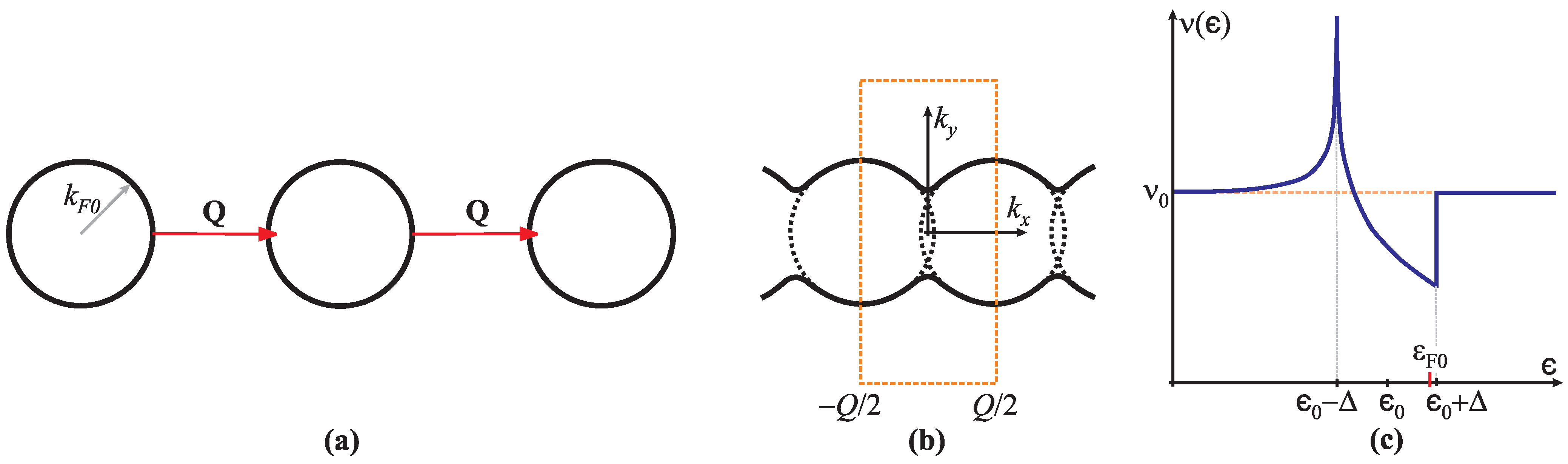
2.1. Model

We assume a model to address the above-mentioned effects comprising the 2D isotropic metallic electrons in the form of the effective free electron gas (2DEG) coupled to the lattice phonons in terms of the well-known Fröhlich Hamiltonian [17,18]

$$\begin{array}{c}\hfill H=\sum _{\mathbf{k}}\epsilon \left(\mathbf{k}\right)a_{\mathbf{k}}^{†}{a}_{\mathbf{k}}+\sum _{\mathbf{q}}\hslash \omega \left(\mathbf{q}\right)b_{\mathbf{q}}^{†}{b}_{\mathbf{q}}+\frac{1}{\sqrt{A}}\sum _{\mathbf{k},\mathbf{q}}{g}_{\mathbf{q}}{a}_{\mathbf{k}+\mathbf{q}}^{†}{a}_{\mathbf{k}}\left(b_{-\mathbf{q}}^{†}+b_{\mathbf{q}}\right),\end{array}$$

(1)

where $a_{\mathbf{k}}$ and $b_{\mathbf{q}}$ are electron and phonon field annihilation operators at the corresponding wave vectors $\mathbf{k}$ and $\mathbf{q}$, respectively. $\epsilon \left(\mathbf{k}\right)={\hslash }^2{\left|\mathbf{k}\right|}^2/2m$ is the initial electron dispersion, with the effective mass m, while $\omega \left(\mathbf{q}\right)$ is the dispersion of the corresponding acoustic phonons coupled to the electronic system by the coupling strength $g_{\mathbf{q}}$, and A is the area of the sample. Presumably, a spontaneously arising CDW forms a self-consistent periodic potential with the wave vector $\mathbf{Q}$ and order parameter $\Delta$ proportional to the non-vanishing mean value of the phonon operator $\langle b_{\mathbf{Q}}\rangle$, i.e., to the ”frozen”, zero-frequency lattice deformation. The minimal zero-temperature analytical model describing the system appears to be given by the Hamiltonian (1) treated within the mean-field approximation [5], i.e.,

$$\begin{array}{c}\hfill H_{MF}=\sum _{\mathbf{k}}\left[\epsilon \left(\mathbf{k}\right)a_{\mathbf{k}}^{†}{a}_{\mathbf{k}}+\Delta e^{i\Phi }{a}_{\mathbf{k}+\mathbf{Q}}^{†}{a}_{\mathbf{k}}+\Delta e^{-i\Phi }{a}_{\mathbf{k}-\mathbf{Q}}^{†}{a}_{\mathbf{k}}\right]+\frac{A\hslash {\omega }_{\mathbf{Q}}}{2g_{\mathbf{Q}}^2}{\Delta }^2,\end{array}$$

(2)

where the second term $\sim {\Delta }^2$ accounts for the elastic energy of the deformed lattice, while the phase of the order parameter $\Phi$ appears to be irrelevant to the description of the ground state. Diagonalization of the first term yields the electronic bands,

$$\begin{array}{c}\hfill {ϵ}_{\pm }\left(\mathbf{k}\right)=\frac{1}{2}\left[\epsilon (\mathbf{k}-\frac{\mathbf{Q}}{2})+\epsilon (\mathbf{k}+\frac{\mathbf{Q}}{2})\pm \sqrt{{\left(\epsilon (\mathbf{k}-\frac{\mathbf{Q}}{2})-\epsilon (\mathbf{k}+\frac{\mathbf{Q}}{2})\right)}^2+4{\Delta }^2}\right],\end{array}$$

(3)

with the origin of the new Brillouin zone chosen at the point at energy ${ϵ}_0={\hslash }^2{Q}^2/\left(8m\right)$ where the initial dispersions cross and the process of the FS reconstruction takes place due to the finite order parameter $\Delta$ (see Figure 1a,b). The coordinate system of the reciprocal space is chosen so that the ${\widehat{k}}_x-$component is parallel with $\mathbf{Q}$. Two bands appear, with a saddle point at energy ${ϵ}_S={ϵ}_0-\Delta$ in the lower band ${ϵ}_{-}\left(\mathbf{k}\right)$, and an elliptic point at energy ${ϵ}_E={ϵ}_0+\Delta$ in the upper band ${ϵ}_{+}\left(\mathbf{k}\right)$, at $\mathbf{k}=(0,0)$. The most important boundary condition during the FS reconstruction process is the conservation of the number of electrons before and after the reconstruction, i.e., $N_0\left({\epsilon }_{F0}\right)=N_r\left({\epsilon }_F\right)$, where ${\epsilon }_{F0}$ and ${\epsilon }_F$ are the Fermi energies of the system before and after the reconstruction, respectively. Taken per unit area ($A=1$) and assuming the spin degeneracy, $N_0\left({\epsilon }_{F0}\right)=m{\epsilon }_{F0}/\left(\pi {\hslash }^2\right)$ and

$$\begin{array}{c}\hfill N_r\left({\epsilon }_F\right)=\frac{2}{{\pi }^2}{\int }_0^{\frac{Q}{2}}{\left[k_{y-}(k_x;ϵ,Q,\Delta )+k_{y+}(k_x;ϵ,Q,\Delta )\right]}_{ϵ={\epsilon }_F}\mathrm{d}{k}_x,\end{array}$$

(4)

where

$$\begin{array}{c}\hfill k_{y\pm }(k_x;ϵ,Q,\Delta )={\left[\frac{2mϵ}{{\hslash }^2}-{\left(\frac{Q}{2}\right)}^2-k_x^2\mp \sqrt{{\left(Q{p}_x\right)}^2+{\left(\frac{2m\Delta }{{\hslash }^2}\right)}^2}\right]}^{1/2}\end{array}$$

(5)

was obtained from Equation (3). Optimization of the electron conservation condition with respect to the new Fermi energy ${\epsilon }_F$ at given Q and $\Delta$ (to be optimized later) gives ${\epsilon }_F={\epsilon }_{F0}$, i.e., the Fermi energy remains unchanged in the reconstruction process. The density of states (DOS) of the reconstructed system is calculated from Equation (4), taken at energy $ϵ$, as $\nu \left(ϵ\right)=\partial N_r\left(ϵ\right)/\partial ϵ$ and is shown in Figure 1c. It exhibits a pseudo-gap between energies ${ϵ}_S$ and ${ϵ}_U$ (saddle and elliptic points in the lower and upper bands, respectively), with the logarithmic type of van Hove singularity at $ϵ={ϵ}_S$. Formation of the pseudo-gap, due to the reconstruction, vs. initially constant DOS, is the key to the stabilization of the spontaneous CDW as we shall show later. Our analysis shows that only the contribution of the lower band ${ϵ}_{-}\left(\mathbf{k}\right)$ leads to the stabilization of the CDW, i.e., lowering the system energy due to the reconstruction. Thus, for the clarity of presentation, only that band is shown in further consideration regarding the ground state.

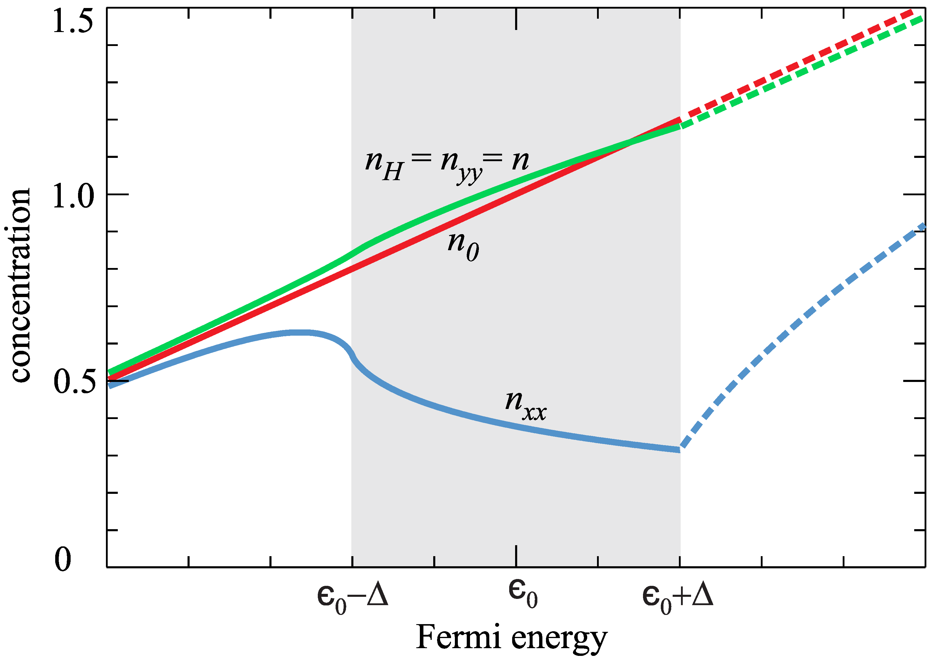
2.2. The CDW Ground State

In order to find the zero-temperature condensation energy of the CDW, first we calculate the electron band energy $E_B=(1/2{\pi }^2)\int {ϵ}_{-}\left(\mathbf{k}\right)\mathrm{d}\mathbf{k}$, where the integral goes from the bottom of the band up to the Fermi surface ${ϵ}_{-}\left(\mathbf{k}\right)={\epsilon }_{F0}$. The CDW condensation energy is the difference between the (band) energy of the initial, unreconstructed system with undeformed lattice, $E_0=m{\epsilon }_{F0}^2/\left(2\pi {\hslash }^2\right)$, and the total energy of the reconstructed state, i.e., the sum of the band energy $E_B$ and elastic energy of the deformed lattice, finally yielding the CDW condensation energy [9]

$$\begin{array}{c}\hfill E_{CDW}=E_0\left[-1+\frac{16}{3\pi k_{F0}^4}{\int }_0^{Q/2}{k}_{y-}^3(k_x;{\epsilon }_{F0},Q,\Delta )\mathrm{d}{k}_x-\frac{1}{\lambda }\frac{{\Delta }^2}{{\epsilon }_{F0}^2}\right],\end{array}$$

(6)

where $k_{F0}=2m{\epsilon }_{F0}/{\hslash }^2$ is the initial Fermi wave vector and $\lambda \equiv m{g}_{\mathbf{Q}}^2/\left(2\pi {\hslash }^3{\omega }_{\mathbf{Q}}\right)$ is the dimensionless electron-phonon coupling constant. Although $\Delta$ and $\lambda$ are in principle dependent on $\mathbf{Q}$, we consider that dependence smooth enough to be neglected in the following optimization procedure. The maximization of $E_{CDW}$ with respect to Q yields the optimal value of the CDW wave vector

$$\begin{array}{c}\hfill Q_{CDW}=2k_{F0}\left(1-\frac{1}{2}\frac{\Delta }{{\epsilon }_{F0}}+\frac{1}{2\sqrt{2}\pi }{\left(\frac{\Delta }{{\epsilon }_{F0}}\right)}^{3/2}+\cdots \right)\end{array}$$

(7)

and position of the Fermi energy with respect to the energy ${ϵ}_0$ (the initial band-crossing energy, i.e., the middle of the pseudo-gap)

$$\begin{array}{c}\hfill {\epsilon }_F={\epsilon }_{F0}={ϵ}_0+\Delta -\frac{1}{\sqrt{2}\pi }\Delta \sqrt{\frac{\Delta }{{ϵ}_0}}+\cdots ,\end{array}$$

(8)

which is apparently inside the pseudo-gap [9]. The value $Q=2k_{F0}$ in expression (7) would mean that the initial FSs exactly touch each other. However, the negative correction $\sim \Delta /{\epsilon }_{F0}$ indicates a small but finite overlap of the initial FSs in the optimal position at which the reconstruction takes place. Taking into account the optimal CDW wave vector (7), we can express the CDW condensation energy (6) in the form of expansion in powers of the small parameter $\Delta /{\epsilon }_{F0}$,

$$\begin{array}{c}\hfill E_{CDW}=E_0\left[\left(\frac{1}{{\lambda }_c}-\frac{1}{\lambda }\right){\left(\frac{\Delta }{{\epsilon }_{F0}}\right)}^2-\frac{1}{\pi }{\left(\frac{\Delta }{{\epsilon }_{F0}}\right)}^3+\cdots \right],\end{array}$$

(9)

where

$$\begin{array}{c}\hfill {\lambda }_c\equiv {\left(1+\frac{2}{\pi }\right)}^{-1}\approx 0.611.\end{array}$$

(10)

Maximization of the condensation energy with respect to the order parameter $\Delta /{\epsilon }_{F0}$ yields a stable solution with a finite value of the order parameter

$$\begin{array}{c}\hfill {\Delta }_{CDW}=\frac{2\pi }{3}\left(\frac{1}{{\lambda }_c}-\frac{1}{\lambda }\right){\epsilon }_{F0},\end{array}$$

(11)

for which $E_{CDW}$ is positive and maximal, provided $\lambda >{\lambda }_c$ [9]. The CDW ground state is, therefore, stable if the electron–phonon coupling is larger than the critical value ${\lambda }_c$ determined by the details of the system, given for this model by expression (10). It has been predicted that such CDW would have even been enhanced by the external magnetic field perpendicular to the sample [11]. It has also been shown that depending on the effective dimensionality $\mathcal{D}$ of the system, the required critical coupling ${\lambda }_c$ is continuously reduced for $\mathcal{D}<2$, reaching zero for $\mathcal{D}=1$ (it coincides with the nesting case described by the Peierls scenario), and is increased for $\mathcal{D}>2$ [10].

2.3. DC Transport and Magnetotransport Coefficients

A rather easy way to experimentally detect changes on the FS, e.g., its topological reconstruction, is by measuring characteristic signatures in electrical DC transport coefficients, such as the concentration of carriers. We distinguish three types of electron concentrations: total and effective concentration in the DC transport, and the Hall concentration in magnetotransport. Within the present model, these concentrations are derived as functions of the Fermi energy ${\epsilon }_F$. Assuming the position of the Fermi energy inside the pseudo-gap (see Equation (8)), only the lower band ${ϵ}_{\mathbf{k}}={ϵ}_{-}\left(\mathbf{k}\right)$ contributes in the following calculations. The total concentration of electrons is defined as

$$\begin{array}{c}\hfill n=\frac{2}{A}\sum _{\mathbf{k}}{f}_{\mathbf{k}},\end{array}$$

(12)

where $f_{\mathbf{k}}$ is the Fermi distribution, with the reconstructed dispersion ${ϵ}_{\mathbf{k}}$ entering as its argument, and A is the aforementioned area of the sample.

Next, there is an effective concentration of electrons $n_{\alpha \alpha }$, which depends on the direction $\alpha$ with respect to the reconstruction wave vector. That is the concentration found in the Drude conductivity formula. It can be written in two equivalent forms

$$\begin{array}{c}\hfill n_{\alpha \alpha }=-\frac{2}{A}\sum _{\mathbf{k}}{m}_e{v}_{\alpha \mathbf{k}}{v}_{\alpha \mathbf{k}}\frac{\partial f_{\mathbf{k}}}{\partial {ϵ}_{\mathbf{k}}}=\frac{2}{A}\sum _{\mathbf{k}}{M}_{\alpha \alpha \mathbf{k}}{f}_{\mathbf{k}},\end{array}$$

(13)

where $v_{\alpha \mathbf{k}}=(1/\hslash )(\partial {ϵ}_{\mathbf{k}}/\partial k_{\alpha })$ is the electron group velocity and $M_{\alpha \beta \mathbf{k}}$ is the dimensionless reciprocal effective mass tensor

$$\begin{array}{c}\hfill M_{\alpha \beta \mathbf{k}}=\frac{m_e}{{\hslash }^2}\frac{{\partial }^2{ϵ}_{\mathbf{k}}}{\partial k_{\alpha }\partial k_{\beta }}\end{array}$$

(14)

($m_e$ is the electron mass).

Finally, there is the so-called Hall concentration $n_H$ which defines the Hall coefficient in a (vanishing) magnetic field perpendicular to the sample plane. It is defined as

$$\begin{array}{c}\hfill n_H=\frac{n_{xx}{n}_{yy}}{n_{xy}},\end{array}$$

(15)

where the diagonal components $n_{\alpha \alpha }$ are defined in Equation (13), and the mixed component $n_{xy}$ is equal to

$$\begin{array}{c}\hfill n_{xy}=-\frac{2}{A}\sum _{\mathbf{k}}{m}_e\left(v_{x\mathbf{k}}{v}_{y\mathbf{k}}{M}_{xy\mathbf{k}}-v_{x\mathbf{k}}{v}_{x\mathbf{k}}{M}_{yy\mathbf{k}}\right)\frac{\partial f_{\mathbf{k}}}{\partial {ϵ}_{\mathbf{k}}}.\end{array}$$

(16)

For this particular model, with bands given by the Equation (3), it is not difficult to see that $M_{xy\mathbf{k}}=0$ and $M_{yy\mathbf{k}}=1$. In this case, by comparing Equation (16) with (13), we see that $n_{xy}=n_{xx}$ and, correspondingly, we get $n_H=n_{yy}=n$, i.e., the Hall concentration equals to the total one. Concentrations of carriers are shown in Figure 2.

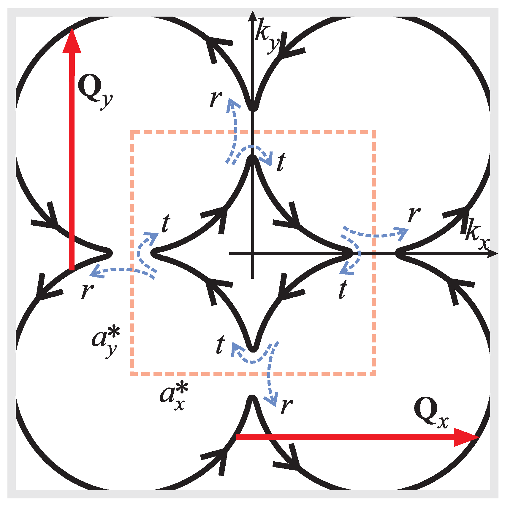
2.4. Magnetotransport in the System Reconstructed by the Bi-Axial CDW under Magnetic Breakdown Conditions

In order to construct a qualitative model addressing the underlying mechanism of the magnetotransport properties observed in some real systems [14,15,16], in which the FS is reconstructed by the checkerboard-like bi-axial CDW, we propose the 2D net of isotropic, circular FSs related by the CDW potential in two perpendicular directions (see Figure 3) analogously to the scenario from the first subsection. Magnetic field $\mathbf{B}=(0,0,B)$ is applied perpendicular to the sample plane. The Fermi surface $ϵ(k_x,k_y)={\epsilon }_F$, after reconstruction by such CDW, consists of the diamond-shaped pockets. The magnetic field causes magnetic breakdown (MB), the quantum tunneling of electrons between close trajectories at the same energy due to the overlap of their wave functions, through the MB-regions where these pockets are close to each other, i.e., in the reconstruction region. Magnetic breakdown in the MB-region is characterized by a probability amplitude $t\left(B\right)$ to pass through it, and a probability amplitude $r\left(B\right)$ to be scattered back on it, related by the unitarity constraint ${\left|t\right|}^2+{\left|r\right|}^2=1$. Depending on t and r, which depend on the magnetic field, the electron can perform a semiclassical motion in three qualitatively different manners: (a) for $\left|t\right|\to 1$, electrons move along the hole-like diamond-shaped orbits; (b) for $\left|r\right|\to 1$, electrons move along the electron-like circular orbits; (c) for $\left|t\right|\sim \left|r\right|$, electrons move freely in $x-$ and $y-$directions, randomly scattering on impurities as if there is effectively no magnetic field. However, for all the three described cases, it is essential to emphasize that the magnetic field should be strong enough to preserve the coherent magnetic breakdown picture, i.e., the Larmor radius should be considerably larger than the electron mean free path due to the impurity scattering. The quantum-mechanical description within the reconstruction region [19,20,21,22] gives the MB tunneling probability

$$\begin{array}{c}\hfill {\left|t\right|}^2\approx 1-exp\left[-\frac{{\Delta }^2}{\hslash {\omega }_c{\epsilon }_F}\sqrt[3]{\frac{{\epsilon }_F}{\hslash {\omega }_c}}\right],\end{array}$$

(17)

where ${\omega }_c\equiv eB/m$ is the cyclotron frequency ($\hslash {\omega }_c$ is then ”magnetic energy”), e is the (absolute) electron charge. One immediately notices that for the given ”nearly touching” FSs configuration, the exponent has an additional large factor, i.e., the third root of the ratio of the Fermi energy and magnetic energy, compared with the standard Blount’s result [23] obtained for the significant crossing of the FSs. It is the result of the peculiar band topology in the reconstruction region.

The semiclassical motion of electrons between the MB-regions is described by the Lifshitz–Onsager Hamiltonian [24,25] which, choosing the Landau gauge of the vector potential $\mathbf{A}=(-By,0,0)$, leads to the Schrödinger equation in the reciprocal space

$$\begin{array}{c}\hfill {\epsilon }_{\alpha }\left(K_x+i\frac{b_B^2}{\hslash }\frac{\mathrm{d}}{\mathrm{d}{k}_y},k_y\right)G_{\alpha }(K_x,k_y)=ϵG_{\alpha }(K_x,k_y),\end{array}$$

(18)

where ${\epsilon }_{\alpha }(k_x,k_y)$ is the initial electron dispersion which is shifted to the position corresponding to the trajectory $\alpha$ between the bounding MB-regions, $b_B=e\hslash B$ is the ”magnetic length”, $(\hslash K_x,\hslash K_y)$ is the conserved generalized momentum of the semiclassical motion of the electron, $ϵ$ is the eigenvalue of energy. The semiclassical eigenfunctions are

$$\begin{array}{c}\hfill G_{\alpha }(K_x,k_y)=\frac{A_{\alpha }}{\sqrt{v_x^{\left(\alpha \right)}}}exp\left[i\frac{{\hslash }^2}{b_B^2}\left(K_x{k}_y+{\int }_0^{k_y}{k}_x^{\left(\alpha \right)}(k_y^{\prime };{\epsilon }_F)\mathrm{d}{k}_y^{\prime }\right)\right],\end{array}$$

(19)

where $A_{\alpha }$ is the corresponding amplitude, $v_x^{\left(\alpha \right)}$ is the semiclassical velocity component, while the integral in the exponent is the semiclassical phase (area enclosed by the trajectory in the reciprocal space, i.e., the ”action”). Wave functions $G_{\alpha }$ along each trajectory $\alpha$ are connected by the $2\times 2$ unitary scattering matrix, the so-called MB matrix consisting of t and r amplitudes, that relate incoming and outgoing waves in the MB-region. They obey the periodicity conditions imposed by the translation operators ${\widehat{T}}_{x,y}$ in $x-$ and $y-$direction in the reciprocal space by the reciprocal lattice constants $a_x^{*}$ and $a_y^{*}$ respectively, i.e.,

$$\begin{array}{c}\hfill {\widehat{T}}_x{G}_{\alpha }\left(\mathbf{k}\right)={\mathrm{e}}^{i({\hslash }^2{K}_y{a}_x^{*}/b_B^2)}{G}_{\alpha }\left(\mathbf{k}\right),\\ \hfill {\widehat{T}}_y{G}_{\alpha }\left(\mathbf{k}\right)={\mathrm{e}}^{i({\hslash }^2{K}_x{a}_y^{*}/b_B^2)}{G}_{\alpha }\left(\mathbf{k}\right).\end{array}$$

(20)

Solving the system of equations coupling the $A_{\alpha }$ amplitudes within MB-nodes, one obtains the determinant of the system

$$\begin{array}{c}\hfill D(ϵ,\mathbf{K})=sin\left[\frac{{\hslash }^2{S}_{\diamond }\left(ϵ\right)}{2b_B^2}+2\chi \right]+\left|tr\right|\left\{sin\left[\frac{{\hslash }^2{a}_y^{*}{K}_x}{b_B^2}+\mu -\eta \right]+sin\left[\frac{{\hslash }^2{a}_x^{*}{K}_y}{b_B^2}-\mu -\eta \right]\right\},\end{array}$$

(21)

where $S_{\diamond }\left(ϵ\right)=a_x^{*}{a}_y^{*}-2\pi mϵ/{\hslash }^2$ is the area of the diamond-shaped orbit in reciprocal space at energy $ϵ$, while $\mu$, $\eta$, and $\chi$ are phases of the probability amplitudes t, r, and the MB-matrix, respectively [13]. The system is consistent under the particular condition ${\hslash }^2{a}_x^{*}{a}_y^{*}/\left(2b_B^2\right)=2\pi n$, $n\in \mathcal{Z}$, which appears to be analog of the well-known Zak–Hofstdater condition of magnetic flux quantization through the unit cell [26,27], here appearing in the reciprocal space. The dispersion law of the system under the coherent MB regime is then $D(ϵ,\mathbf{K})=0$. Electronic spectrum

$$\begin{array}{c}\hfill {ϵ}_s(K_x,K_y)=\hslash {\omega }_B\left\{s+\frac{2\chi }{\pi }+\frac{{(-1)}^s}{\pi }arcsin\left[\left|tr\right|\left(sin\left(\frac{{\hslash }^2{a}_y^{*}{K}_x}{b_B^2}+\mu -\eta \right)+sin\left(\frac{{\hslash }^2{a}_x^{*}{K}_y}{b_B^2}-\mu -\eta \right)\right)\right]\right\}\end{array}$$

(22)

is obtained directly from the dispersion law, where $s=0,1,2,...$ is the new ”magnetic band” index. The width of magnetic bands,

$$\begin{array}{c}\hfill W\left(B\right)=\frac{2}{\pi }arcsin\left[2\left|t\right(B\left)r\right(B\left)\right|\right]\hslash {\omega }_c,\end{array}$$

(23)

and gaps between them, $\hslash {\omega }_c-W\left(B\right)$, depend on magnetic field. They are crucially determined by the $\left|t\right(B\left)r\right(B\left)\right|$ product which vanishes in the limit of very low and very high fields while attaining the maximal value of $1/2$ in the regime of moderate field (these regimes depend on the details of the particular system, such as $\Delta$, ${\epsilon }_F$, and FS shape).

The magnetoconductivity operates in two essentially different regimes depending on the relation between the magnetic bandwidth $W\left(B\right)$ and level broadening due to the impurity scattering $\hslash {\omega }_0$ (${\omega }_0\sim {\tau }_0^{-1}$ is the scattering rate, ${\tau }_0$ is the impurity scattering relaxation time): (1) for $W\left(B\right)\ll \hslash {\omega }_0$, the spectrum is effectively a set of Landau levels, leading to the semiclassical motion around diamond-shaped or circular orbits, depending on t and r; (2) for $W\left(B\right)\gg \hslash {\omega }_0$, the group velocity in both directions $\mathbf{v}=(1/\hslash ){▿}_{\mathbf{K}}{ϵ}_s\left(\mathbf{K}\right)$ is large, particles move along ”diamonds” and ”circles”, tunneling between them. The Hall coefficient is calculated in the standard way, in terms of the components of the magnetoconductivity tensor $\widehat{\sigma }$, i.e.,

$$\begin{array}{c}\hfill R_H=\frac{{\sigma }_{xy}}{({\sigma }_{xx}{\sigma }_{yy}+{\sigma }_{xy}^2)B}.\end{array}$$

(24)

The case (1), $W\left(B\right)\ll \hslash {\omega }_0$, is rather well-known from the theory of metals [28], yielding the following result [13]:

(a)

In a relatively weak field with small MB effect, $\left|t\right(B\left)\right|\to 1$ ($\left|r\left(B\right)\right|\ll {\omega }_0/{\omega }_c\ll 1$) carriers move along the hole-like diamond-shaped trajectories, the magnetoconductivity is

$$\begin{array}{ccc}\hfill {\sigma }_{xx}^{\left(h\right)}={\sigma }_{yy}^{\left(h\right)}& =& \frac{{\sigma }_0^{\left(h\right)}}{{\left({\tau }_0{\omega }_c\right)}^2}\sim \frac{1}{B^2},\hfill \\ \hfill {\sigma }_{xy}^{\left(h\right)}=-{\sigma }_{yx}^{\left(h\right)}& =& \frac{n^{\left(h\right)}e}{B}\sim \frac{1}{B},\hfill \\ \hfill R_H& =& \frac{1}{e{n}^{\left(h\right)}}.\hfill \end{array}$$

(25)

(b)

In a relatively strong field with a large MB effect, $\left|t\right(B\left)\right|\to 0$ ($\left|t\left(B\right)\right|\ll {\omega }_0/{\omega }_c\ll 1$) carriers move along the electron-like circular trajectories, the magnetoconductivity is

$$\begin{array}{ccc}\hfill {\sigma }_{xx}^{\left(e\right)}={\sigma }_{yy}^{\left(e\right)}& =& \frac{{\sigma }_0^{\left(e\right)}}{{\left({\tau }_0{\omega }_c\right)}^2}\sim \frac{1}{B^2},\hfill \\ \hfill {\sigma }_{xy}^{\left(e\right)}=-{\sigma }_{yx}^{\left(e\right)}& =& -\frac{n^{\left(e\right)}e}{B}\sim \frac{1}{B},\hfill \\ \hfill R_H& =& -\frac{1}{e{n}^{\left(e\right)}}.\hfill \end{array}$$

(26)

Here, ${\sigma }_0^{(e,h)}=n^{(e,h)}{e}^2{\tau }_0/m$ is the conductivity of electrons $\left(e\right)$, or holes $\left(h\right)$, in the absence of magnetic field, while $n^{\left(e\right)}=\pi k_{F0}^2/{\left(2\pi \right)}^2$ is the concentration of electrons, and $n^{\left(h\right)}=[{\left(a^{*}\right)}^2-\pi k_{F0}^2]/{\left(2\pi \right)}^2$ the concentration of holes ($k_{F0}$ is the Fermi wave vector). We consider $a_x^{*}=a_y^{*}\equiv a^{*}$ and equal effective masses m for electrons and holes for the sake of simplicity.

In the case (2), $W\left(B\right)\gg \hslash {\omega }_0$, the magnetoconductivity tensor is calculated using the density matrix in the linear approximation, i.e., $\widehat{\rho }=f_0\left({\widehat{H}}_0\right)+{\widehat{\rho }}^{\left(1\right)}$, for electrons under electric field $\mathbf{E}$, $f_0$ is the Fermi distribution function. The equation to determine the nonequilibrium correction ${\widehat{\rho }}^{\left(1\right)}$ reads

$$\begin{array}{c}\hfill \frac{1}{i\hslash }\left[{\widehat{H}}_0,{\widehat{\rho }}^{\left(1\right)}\right]+\frac{{\widehat{\rho }}^{\left(1\right)}}{{\tau }_0}=-\frac{e\mathbf{E}}{i\hslash }\left[\widehat{\mathbf{r}},f_0\left({\widehat{H}}_0\right)\right],\end{array}$$

(27)

where ${\tau }_0$ is the impurity scattering relaxation time and ${\widehat{H}}_0$ is the one-particle effective Hamiltonian satisfying the Schrodinger equation ${\widehat{H}}_0|n,\mathbf{K}\rangle ={ϵ}_n\left(\mathbf{K}\right)|n,\mathbf{K}\rangle$, with Bloch eigen-functions $|n,\mathbf{K}\rangle$ and eigen-energy ${ϵ}_n\left(\mathbf{K}\right)$ defined by the dispersion law $D(ϵ,\mathbf{K})=0$.

Taking into account the fact that both projections of velocity are finite, $v_x\ne 0$ and $v_y\ne 0$, one finds the density matrix nonequilibrium correction

$$\begin{array}{c}\hfill {\rho }_{\kappa {\kappa }^{\prime }}^{\left(1\right)}=e\mathbf{E}\frac{i\hslash {\mathbf{v}}_{\kappa {\kappa }^{\prime }}}{{ϵ}_{\kappa }-{ϵ}_{{\kappa }^{\prime }}+i\hslash {\omega }_0}\frac{f_0\left({ϵ}_{\kappa }\right)-f_0\left({ϵ}_{{\kappa }^{\prime }}\right)}{{ϵ}_{\kappa }-{ϵ}_{{\kappa }^{\prime }}},\end{array}$$

(28)

where $\kappa \equiv (\mathbf{K},n)$ and ${\mathbf{v}}_{\kappa {\kappa }^{\prime }}=(\partial {ϵ}_{\kappa }/\hslash \partial \mathbf{K})\delta (\mathbf{K}-{\mathbf{K}}^{\prime }){\delta }_{n,n^{\prime }}$ are the velocity matrix elements. The magnetoconductivity tensor $\widehat{\sigma }$ is obtained by expressing the velocity components in its definition in terms of $D(ϵ,\mathbf{K})$, using the method developed by Slutskin for complicated spectra under the MB conditions [29], i.e.,

$$\begin{array}{c}\hfill {\sigma }_{ij}=-2e^2{\tau }_0\int \mathrm{d}ϵ\frac{\partial f_0}{\partial ϵ}\int \frac{\mathrm{d}\mathbf{K}}{{(2\pi \hslash )}^2}\frac{\frac{\partial D}{\partial K_i}\frac{\partial D}{\partial K_j}}{|\frac{\partial D}{\partial ϵ}|}\delta \left[D(ϵ,\mathbf{K})\right].\end{array}$$

(29)

Using Equation (21) and the periodicity of the fast-oscillating integrand, in the sense that we kept only the constant term in its double-Fourier expansion, we obtain components of the magnetoconductivity tensor and the Hall coefficient [13]

$$\begin{array}{ccc}\hfill {\sigma }_{xx}& =& -e^2{\tau }_0\frac{{\left(a_y^{*}\right)}^2}{{\pi }^{4}m{\hslash }^2}\left[\frac{1}{2\pi }\left(\frac{a_x^{*}{a}_y^{*}}{2b_B^2}\right)\right]\int \mathrm{d}ϵ\frac{\partial f_0/\partial ϵ}{|cos{\Phi }_{\diamond }|}{\int }_{-\pi }^{+\pi }\mathrm{d}\phi \sqrt{{\left|tr\right|}^2-{\left(\left|tr\right|cos\phi -sin{\Phi }_{\diamond }\left(ϵ\right)\right)}^2}\hfill \\ & \times & \Theta \left[{\left|tr\right|}^2-{\left(\left|tr\right|cos\phi -sin{\Phi }_{\diamond }\left(ϵ\right)\right)}^2\right],\hfill \\ \hfill {\sigma }_{xy}& =& 0,\hfill \\ \hfill R_H& =& 0,\hfill \end{array}$$

(30)

where ${\Phi }_{\diamond }\left(ϵ\right)\equiv {\hslash }^2{S}_{\diamond }\left(ϵ\right)/\left(2b_B^2\right)+\chi$ and $\Theta$ is the Heaviside unit-step function. The other two components, ${\sigma }_{yy}$ and ${\sigma }_{yx}$, are simply obtained from the above expression by changing the indices $x\leftrightarrow y$. Apparently, in this regime, the diagonal components of the conductivity tensor, ${\sigma }_{xx}$ and ${\sigma }_{yy}$, are fast-oscillating functions of the magnetic field, with period determined by the size of the carrier pocket at the Fermi surface $S_{\diamond }\left(ϵ\right)$ (see Figure 4), while the Hall conductivity ${\sigma }_{xy}$ vanishes. The peculiar absence of the Hall effect, in spite of the rather large magnetic field, is exact within the applied approximations, it is a property of the symmetry of the integral.

The Hall coefficient is essentially determined by the value of $t\left(B\right)r\left(B\right)$ product, covering the above-elaborated cases (1) a, b, and (2) (see Figure 5). In the regime of the predominant magnetic breakdown, carriers move along the (parts of) circular trajectories, thus the carrier concentrations $n^{\left(e\right)}$ and $n^{\left(h\right)}$ are close to their free-electron values.

3. Discussion

We present the review of our results related to the novel mechanism of charge density wave (CDW) stabilization in a two-dimensional metallic system with isotropic pockets constituting the initial Fermi surface, where electrons are coupled to phonons via standard Fröhlich coupling. The presented results cover the mechanism of the ground state stabilization, the DC transport coefficients (total and effective concentration of carriers as well as the Hall coefficient) in the system reconstructed by a uni-axial CDW, and the magnetotransport properties (magnetoconductivity tensor and Hall coefficient) of the system reconstructed by a bi-axial CDW.

Due to the isotropy of the Fermi pockets, the paradigmatic mechanism of the CDW ground state stabilization based on “nesting” is not applicable. Here, the CDW ground state stabilization is based on the condensation energy gain due to the topological reconstruction of the Fermi surface, which opens the pseudo-gap in the one-electron density of states, with the Fermi energy inside it. It leads to redistribution of the occupied initial electron states to lower energies due to the presence of the van Hove singularity at the lower “boundary” of the pseudo-gap. This mechanism is self-consistent in the sense that electron density gets modulated exactly in the way to maximize the CDW condensation energy. The wave vector of the self-consistent CDW potential relates the initial electron pockets at the Fermi surface, i.e., electron states get scattered by the potential, exactly to perform the above-described reconstruction of the Fermi surface. The optimal wave vector is such to bring the pockets into a very small overlap, of the order of size of the pocket multiplied by the ratio of the CDW order parameter and the Fermi energy of the system. The mechanism yields a finite order parameter of the CDW ground state if the electron–phonon coupling is larger than the critical value, for the considered system it is roughly equal to $0.6$ (in the standard dimensionless form).

The reconstruction process by the uni-axial CDW leaves the “signature” in the DC transport coefficients. That signature is clearly visible in the considerable reduction of the longitudinal component (with respect to the reconstruction vector) of the carrier effective concentration, the one entering the Drude DC conductivity, within the pseudo-gap. The perpendicular component and the Hall concentration are equal to the total concentration of carriers.

The magnetoconductivity tensor is calculated for the system, with initially circular pockets at the Fermi surface, reconstructed by the bi-axial, checkerboard-like CDW, forming a 2D net of diamond-shaped pockets. In the regime of the coherent magnetic breakdown (the Larmor radius is considerably larger than the electron mean free path) due to the perpendicular magnetic field B, three qualitatively different regimes of magnetoconductivity behavior appear depending on its strength:

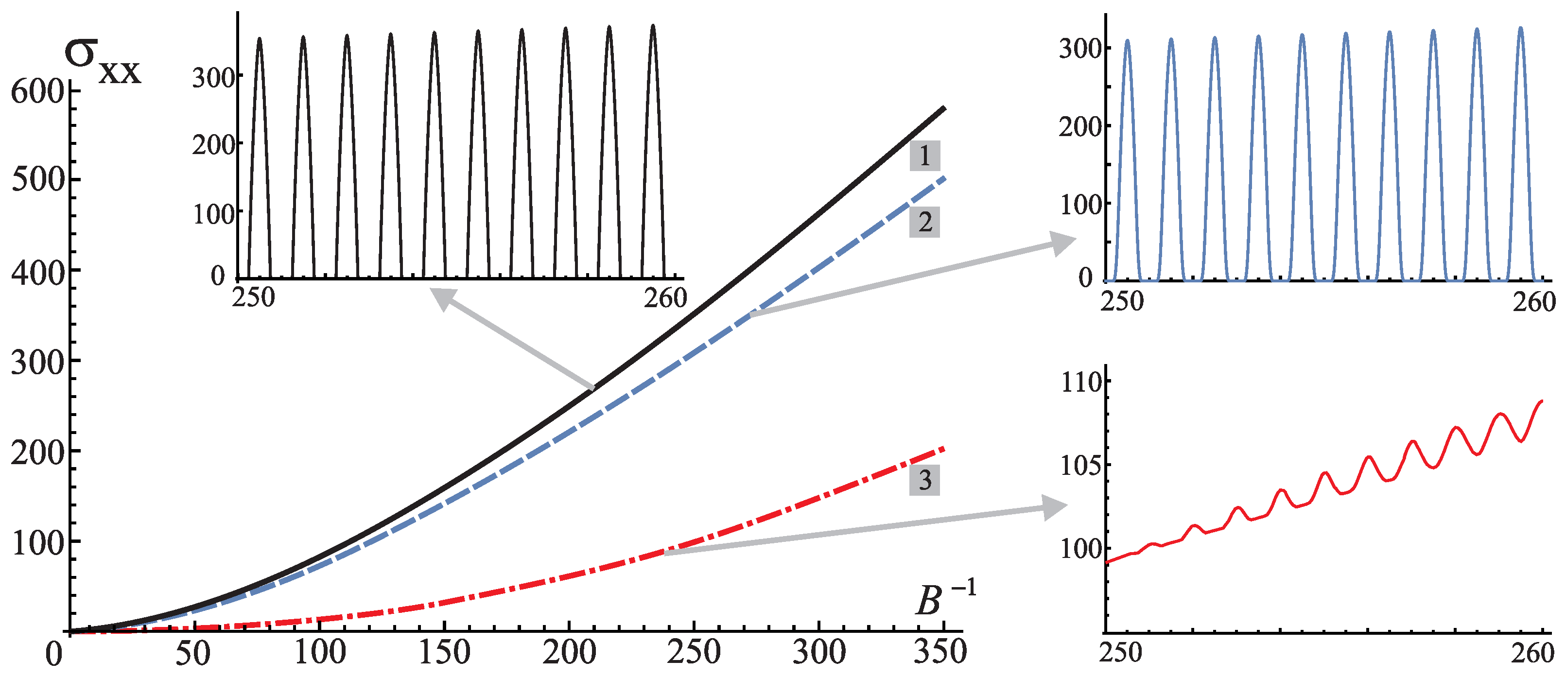
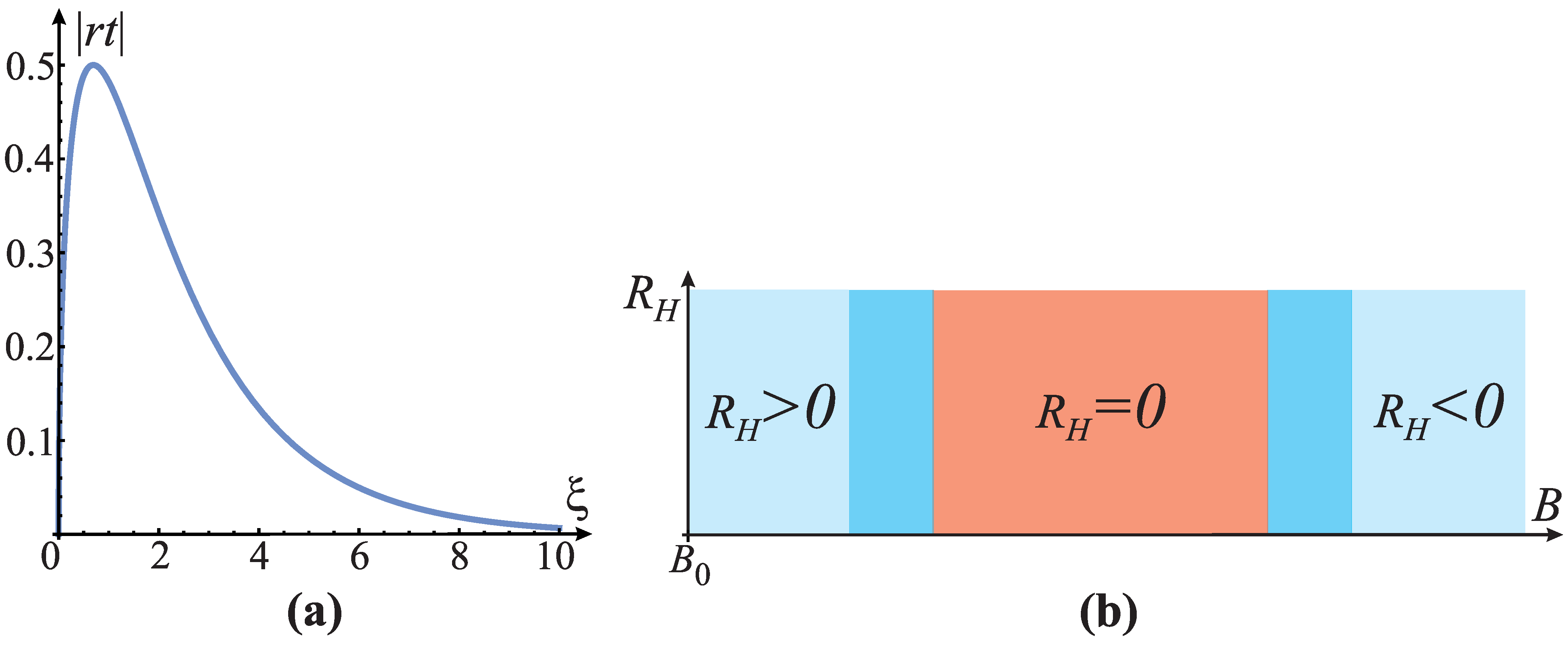
(1)

In the low-field regime with rather weak magnetic breakdown, electrons move along the hole-like semiclassical orbits around the diamond-shaped pockets, with a positive Hall coefficient.

(2)

In the high-field regime with very strong magnetic breakdown, electrons move along the electron-like semiclassical orbits consisting of parts of the diamond-shaped pockets recreating the initial, pre-reconstruction circular orbits, with a negative Hall coefficient. Both (1) and (2) are valid in the limit of very narrow magnetic bands with respect to the broadening of the level due to the impurity scattering, essentially reducing to the Landau level physics with standard diagonal magnetoconductivity proportional to $1/B^2$, and Hall conductivity to $1/B$.

(3)

In the regime of the moderate magnetic field so that magnetic bands (due to magnetic breakdown) are considerably wider compared to the level broadening due to the impurity scattering, the diagonal components of magnetoconductivity exhibit strong quantum oscillations, periodic in the inverse magnetic field, with period determined by the size of pockets forming the Fermi surface. The Hall conductivity (and consequently the Hall coefficient) vanishes. Electrons move freely in this regime (up to the scattering on impurities) over the 2D net, along the arcs forming the diamond-shaped orbits and, in turn, the circular ones, as if there is effectively no magnetic field. Taken together, varying the magnetic field, regimes (1)–(3) exhibit a change of sign of the Hall coefficient, with a finite interval of its vanishing between the two with opposite signs. The presented results are based on the simplified analytical model revealing the background mechanisms and their expected signatures in experiments. It is not material-specific; therefore, it proves the existence of the effect being accurate to the order of magnitude, but presents a solid foundation for the more accurate approaches, such as the ab initio studies which are material-specific, sometimes of high accuracy, but can hardly reveal novel mechanisms. Combined together, the quantitative studies of specific materials, in which the above-counted effects were observed (e.g., high-T${}_c$ superconducting cuprates, transition metal dichalcogenides, etc.), may have a great perspective.

References

- Grüner, G. The dynamics of charge-density waves. Rev. Mod. Phys. 1988, 60, 1129–1181. [Google Scholar] [CrossRef]
- Pouget, J.P. Chapter 3 Structural Instabilities. Semicond. Semimet. 27, 87–214 (1988). Pouget, J.P. Structural Aspects of the Bechgaard and Fabre Salts: An Update. Crystals 2012, 2, 466–520. [Google Scholar] [CrossRef]
- Thorne, R.E. Charge-Density-Wave Conductors. Phys. Today 1996, 49, 42–47. [Google Scholar] [CrossRef]
- Peierls, R.E. Quantum Theory of Solids; Clarendon Press: Oxford, UK, 1955; p. 108. [Google Scholar]
- Sólyom, J. Fundamentals of the Physics of Solids, Vol. III; Springer: Berlin/Heidelberg, Germany, 2010; Chapter 33. [Google Scholar]
- Tranquada, J.M.; Sternlieb, B.J.; Axe, J.D.; Nakamura, Y.; Uchida, S. Evidence for stripe correlations of spins and holes in copper oxide superconductors. Nature 1995, 375, 561–563. [Google Scholar] [CrossRef]
- Wu, T.; Mayaffre, H.; Krämer, S.; Horvatić, M.; Berthier, C.; Hardy, W.N.; Liang, R.; Bonn, D.A.; Julien, M.-H. Magnetic-field-induced charge-stripe order in the high-temperature superconductor YBa2Cu3Oy. Nature 2011, 477, 191–194. [Google Scholar] [CrossRef] [PubMed]
- Fradkin, E.; Kivelson, S. Ineluctable complexity. Nat. Phys. 2012, 8, 864–866. [Google Scholar] [CrossRef]
- Kadigrobov, A.M.; Bjeliš, A.; Radić, D. Topological instability of two-dimensional conductors. Phys. Rev. B 2018, 97, 235439. [Google Scholar] [CrossRef]
- Spaić, M.; Radić, D. Onset of pseudogap and density wave in a system with a closed Fermi surface. Phys. Rev. B 2021, 103, 075133. [Google Scholar] [CrossRef]
- Kadigrobov, A.M.; Radić, D.; Bjeliš, A. Density wave and topological reconstruction of an isotropic two-dimensional electron band in external magnetic field. Phys. Rev. B 2019, 100, 115108. [Google Scholar] [CrossRef]
- Rukelj, Z.; Radić, D. DC and optical signatures of the reconstructed Fermi surface for electrons with parabolic band. New J. Phys. 2022, 24, 053024. [Google Scholar] [CrossRef]
- Kadigrobov, A.M.; Bjeliš, A.; Radić, D. Magnetoconductivity of a metal with a closed Fermi surface reconstructed by a biaxial density wave. Phys. Rev. B 2021, 104, 155143. [Google Scholar] [CrossRef]
- Doiron-Leyraud, N.; Proust, C.; LeBoeuf, D.; Levallois, J.; Bonnemaison, J.B.; Liang, R.; Taillefer, L. Quantum oscillations and the Fermi surface in an underdoped high-Tc superconductor. Nature 2007, 447, 565–568. [Google Scholar] [CrossRef] [PubMed]
- LeBoeuf, D.; Doiron-Leyraud, N.; Vignolle, B.; Sutherland, M.; Ramshaw, B.J.; Levallois, J.; Daou, R.; Laliberté, F.; Cyr-Choinière, O.; Chang, J.; et al. Lifshitz critical point in the cuprate superconductor YBa2Cu3Oy from high-field Hall effect measurements. Phys. Rev. B 2011, 83, 054506. [Google Scholar]
- Shi, Z.; Baity, P.G.; Terzic, J.; Pokharel, B.K.; Sasagawa, T.; Popović, D. Magnetic field reveals vanishing Hall response in the normal state of stripe-ordered cuprates. Nat. Commun. 2021, 12, 3724. [Google Scholar] [CrossRef] [PubMed]
- Fröhlich, H.; Pelzer, H.; Zienau, S. Properties of slow electrons in polar materials. Phil. Mag. 1950, 41, 221–242. [Google Scholar] [CrossRef]
- Fröhlich, H. Electrons in lattice fields. Adv. Phys. 1954, 3, 325–361. [Google Scholar] [CrossRef]
- Kadigrobov, A.; Bjeliš, A.; Radić, D. Peierls-type structural phase transition in a crystal induced by magnetic breakdown. Eur. Phys. J. B 2013, 86, 276. [Google Scholar] [CrossRef][Green Version]
- Kadigrobov, A.M.; Radić, D.; Bjeliš, A. Magnetic breakdown in an array of overlapping Fermi surfaces. Phys. Condens. Matter 2015, 460, 248–252. [Google Scholar] [CrossRef]
- Kadigrobov, A.M.; Slutskin, A.A.; Vorontsov, S.A. Interband tunneling of the electrons near the phase transition of the 212 order. J. Phys. Chem. Solids 1992, 53, 387–393. [Google Scholar] [CrossRef]
- Fortin, J.Y.; Audouard, A. Transmission and tunneling probability in two-band metals: Influence of magnetic breakdown on the Onsager phase of quantum oscillations. Low Temp. Phys. 2017, 43, 173–185. [Google Scholar] [CrossRef][Green Version]
- Blount, E.I. Bloch Electrons in a Magnetic Field. Phys. Rev. 1962, 126, 1636–1653. [Google Scholar] [CrossRef]
- Lifshitz, I.M.; Kosevich, A.M. On the theory of magnetic susceptibility of metals at low temperatures. Z. Eksp. Teor. Fiz. 1955, 29, 730–742. [Google Scholar]
- Onsager, L. Interpretation of the de Haas-van Alphen effect. Philos. Mag. 1952, 43, 1006–1008. [Google Scholar] [CrossRef]
- Zak, J. Magnetic Translation Group. Phys. Rev. 1964, 134, A1602–A1606. [Google Scholar]
- Hofstadter, D.R. Energy levels and wave functions of Bloch electrons in rational and irrational magnetic fields. Phys. Rev. B 1976, 14, 2239–2249. [Google Scholar] [CrossRef]
- Lifshits, I.M.; Azbel, M.Y.; Kaganov, M.I. Electron Theory of Metals; Consultants Bureau (Plenum): New York, NY, USA, 1973. [Google Scholar]
- Kaganov, M.I.; Slutskin, A.A. Coherent magnetic breakdown. Phys. Rep. 1983, 98, 189–271. [Google Scholar] [CrossRef]
Publisher’s Note: MDPI stays neutral with regard to jurisdictional claims in published maps and institutional affiliations. |
© 2022 by the authors. Licensee MDPI, Basel, Switzerland. This article is an open access article distributed under the terms and conditions of the Creative Commons Attribution (CC BY) license (https://creativecommons.org/licenses/by/4.0/).
Share and Cite
Keran, B.; Grozić, P.; Kadigrobov, A.M.; Rukelj, Z.; Radić, D. DC Transport and Magnetotransport Properties of the 2D Isotropic Metallic System with the Fermi Surface Reconstructed by the Charge Density Wave. Condens. Matter 2022, 7, 73. https://doi.org/10.3390/condmat7040073
Keran B, Grozić P, Kadigrobov AM, Rukelj Z, Radić D. DC Transport and Magnetotransport Properties of the 2D Isotropic Metallic System with the Fermi Surface Reconstructed by the Charge Density Wave. Condensed Matter. 2022; 7(4):73. https://doi.org/10.3390/condmat7040073
Chicago/Turabian StyleKeran, Barbara, Petra Grozić, Anatoly M. Kadigrobov, Zoran Rukelj, and Danko Radić. 2022. "DC Transport and Magnetotransport Properties of the 2D Isotropic Metallic System with the Fermi Surface Reconstructed by the Charge Density Wave" Condensed Matter 7, no. 4: 73. https://doi.org/10.3390/condmat7040073
APA StyleKeran, B., Grozić, P., Kadigrobov, A. M., Rukelj, Z., & Radić, D. (2022). DC Transport and Magnetotransport Properties of the 2D Isotropic Metallic System with the Fermi Surface Reconstructed by the Charge Density Wave. Condensed Matter, 7(4), 73. https://doi.org/10.3390/condmat7040073