On the Husimi Version of the Classical Limit of Quantum Correlation Functions

Abstract

We extend the Husimi (coherent state) based version of linearized semiclassical theories for the calculation of correlation functions to the case of survival probabilities. This is a case that could be dealt with before only by use of the Wigner version of linearized semiclassical theory. Numerical comparisons of the Husimi and the Wigner case with full quantum results as well as with full semiclassical ones will be given for the revival dynamics in a Morse oscillator with and without coupling to an additional harmonic degree of freedom.

1. Introduction

The quest for a simplified description of quantum dynamics of many body systems in terms of classical dynamical input has recently become ever more prominent [1]. A lot of the progress that has been made recently in the quantum optics community for bosonic systems is based on the use of the so-called truncated Wigner approximation [2,3,4].

Along similar lines, in the chemical physics community, a classical Wigner dynamics was introduced early on by Heller [5], with a precursor in reaction rate theory by Miller [6]. Historically, the heuristic introduction of this Wigner method, based on classical trajectories preceded its derivation from a semiclassical initial value representation of the propagator by Cao and Voth [7] by two decades. Nowadays, the classical Wigner method in chemical physics is also referred to as linearized semiclassical initial value representation (LSC-IVR) and is prominently used by the Miller group [8,9,10]. Technically, the LSC-IVR method is much easier to apply than the full semiclassical initial value representation (SC-IVR) of, e.g., Herman and Kluk [11], as it linearizes the phase difference between interfering classical trajectories and does not contain any oscillating terms in the integrand (no sign problem). In addition to the application to (reactive) single surface dynamics, also the application of LSC-IVR to electronically nonadiabatic processes i.e., those involving transitions between different potential energy surfaces was shown by Miller and co-authors [12,13]. Furthermore, LSC-IVRs are close in spirit to the diagonal approximation that is used to calculate the smooth part of the semiclassical spectral density in chaotic systems [14].

Whereas in the pioneering works of the Heller as well as the Miller groups, Wigner transforms in the LSC-IVR are used, a new semiclassical framework, introduced by Antipov, Ye and Ananth [15], based on Husimi functions, see also [16,17], can be tuned to reproduce existing quantum-limit and classical-limit SC approximations to quantum real-time correlation functions. So far, the applicability of the Husimi LSC-IVR is restricted to correlation functions $C_{AB}\left(t\right)=\langle \widehat{A}\widehat{B}\left(t\right)\rangle$ with operators $\widehat{B}$ that do not contain exponential terms [15]. In the present contribution, we will extend the usability of the Husimi based LSC-IVR to the calculation of survival probabilities, that is, we will choose identical (projection) operators $\widehat{A}=\widehat{B}=|\Psi \rangle \langle \Psi |$, where the involved wavefunctions are Gaussians. We will discuss, however, also other more common choices for the operators.

In the course of our investigations, we will show comparisons of numerical results for survival probabilities using three different approaches (Wigner LSC-IVR, Husimi LSC-IVR and full SC-IVR) with the full quantum mechanical results. The system for which we perform the investigations is the Morse oscillator and we will especially focus on the revival phenomenon which is present in the full quantum dynamics. If the Morse oscillator is coupled to a harmonic oscillator (acting as a bath for the system) the revival phenomenon is expected to vanish also in the full quantum result.

This paper is organized as follows. First, in Section 2, general correlation functions will be introduced. Then two possible classical approximations will be discussed and because the Husimi version is less general than the Wigner form, in Section 3, a new approach to the survival probability will be laid out. A comparison of numerical results in Section 4 is followed by discussions and an outlook in Section 5. Detailed analytical calculations of determinants of block matrices whose results are needed in the main text can be found in the Appendix A and Appendix B.

2. Theory

In the following, we will introduce the general form of correlation functions that are to be studied and then we will compare different implementations thereof based on classical trajectories.

2.1. General Correlation Functions

The time correlation function of two arbitrary operators $\widehat{A}$ and $\widehat{B}$ with a (Heisenberg) time-evolved operator $\widehat{B}\left(t\right)$ is defined as

$$\begin{array}{c}\hfill C_{AB}\left(t\right)=\mathrm{Tr}\left[\widehat{A}\widehat{B}\left(t\right)\right]=\mathrm{Tr}\left[\widehat{A}{\mathrm{e}}^{\frac{\mathrm{i}}{\hslash }\widehat{H}t}\widehat{B}{\mathrm{e}}^{-\frac{\mathrm{i}}{\hslash }\widehat{H}t}\right]\end{array}$$

(1)

where $\widehat{H}={\sum }_{i=1}^N\frac{p_i^2}{2m_i}+V\left(\mathbf{q}\right)$ is the Hamiltonian of the system under consideration. This system shall have $2N$ degrees of freedom in phase space, denoted by $(\mathbf{p},\mathbf{q})$.

Dynamic phenomena in complex systems can be described in terms of real-time correlation functions. The general time correlation function has various applications based on the choice of the arbitrary operators $\widehat{A}$ and $\widehat{B}$. Various choices for the operators of the correlation function are as follows:

• $\widehat{A}=|{\Psi }_{\alpha }\rangle \langle {\Psi }_{\alpha }|$, $\widehat{B}=|{\Psi }_{\alpha }\rangle \langle {\Psi }_{\alpha }|$
  $|{\Psi }_{\alpha }\rangle \langle {\Psi }_{\alpha }|$ is a projection operator on initial state $|{\Psi }_{\alpha }\rangle$. This leads to the survival probability which is equivalent to the absolute value squared of the auto-correlation function. In the following, we will assume the initial states to be Gaussian wavefunctions.
• $\widehat{A}=Q^{-1}exp\left\{-\beta \widehat{H}\right\}\widehat{\mathbf{r}}$, $\widehat{B}=\widehat{\mathbf{r}}$,
  where Q is the partition function, $\beta =1/kT$ inverse temperature and $\widehat{\mathbf{r}}$ the position operator. This is the temperature dependent dipole-dipole correlation function used to study IR spectra. Semiclassical investigations for this case have been performed in [16,18,19] in the high temperature limit $\beta \to 0$.
• $\widehat{A}=|{\Psi }_{\alpha }\rangle \langle {\Psi }_{\alpha }|$, $\widehat{B}=|\mathbf{r}\rangle \langle \mathbf{r}|$
  This choice leads to the reduced density. For the case of a Caldeira-Leggett model, the transition to classicality and the blue shift of the system oscillator have been investigated in [20], see also [21].
• $\widehat{A}=|{\Psi }_{\alpha }\rangle \langle {\Psi }_{\alpha }|$, $\widehat{B}=\widehat{x},\widehat{x^2},\cdots$
  Here $\widehat{x}$ is the position operator in one dimension. This choice is used to calculate time-dependent moments.

We will be evaluating the dipole-dipole correlation function and the survival probability using both Wigner LSC-IVR and Husimi LSC-IVR methods in the following subsection.

2.2. Comparison between Wigner LSC-IVR and Husimi LSC-IVR

For the following comparison, we restrict the discussion to the case $N=1$, i.e., a single degree of freedom. The generalization to arbitrary N is straightforward.

In the classical, so-called LSC-IVR employing Wigner functions, the expression for the general time-correlation function is given by [5,7]

$$\begin{array}{c}\hfill C_{AB}^W\left(t\right)=\int \frac{\mathrm{d}p\mathrm{d}q}{2\pi \hslash }{A}_W\left(p,q\right)B_W\left(p_t,q_t\right),\end{array}$$

(2)

where $A_W\left(p,q\right)$ and $B_W\left(p_t,q_t\right)$ are the Wigner-Weyl transforms of operators $\widehat{A}$ and $\widehat{B}$ and $(p_t,q_t)$ are classical trajectories in phase space that evolve from the initial conditions $(p,q)$ according to Hamilton’s equations of motion

$$\begin{array}{c}\hfill {\dot{q}}_t=\frac{\partial H}{\partial p_t}{\dot{p}}_t=-\frac{\partial H}{\partial q_t}.\end{array}$$

(3)

$A_W\left(p,q\right)$ is defined as:

$$\begin{array}{c}\hfill A_W\left(p,q\right)=\int \mathrm{d}\Delta q{\mathrm{e}}^{-\mathrm{i}\frac{p\Delta q}{\hslash }}〈q+\frac{\Delta q}{2}|\widehat{A}|q-\frac{\Delta q}{2}〉.\end{array}$$

(4)

Now in the case of the coherent state based LSC-IVR method employing Husimi functions, the general time-correlation function is given by [15]

$$\begin{array}{c}\hfill C_{AB}^H\left(t\right)=\int \frac{\mathrm{d}p\mathrm{d}q}{2\pi \hslash }{A}_H\left(p,q\right)B_H\left(p_t,q_t\right),\end{array}$$

(5)

where $A_H\left(p,q\right)$ and $B_H\left(p_t,q_t\right)$ are the Husimi transforms of the operators $\widehat{A}$ and $\widehat{B}$. $A_H\left(p,q\right)$ is defined as [22]

$$\begin{array}{c}\hfill A_H\left(p,q\right)=\langle z(p,q)|\widehat{A}|z(p,q)\rangle ,\end{array}$$

(6)

where $|z(p,q)\rangle$ represents a coherent state with width parameter $\tilde{\gamma }$, given in position representation by

$$\begin{array}{c}\hfill \langle x|z(p,q)\rangle ={\left(\frac{\tilde{\gamma }}{\pi }\right)}^{1/4}{\mathrm{e}}^{-\frac{\tilde{\gamma }}{2}{(x-q)}^2+\frac{\mathrm{i}}{\hslash }p(x-q)},\end{array}$$

(7)

with a phase convention slightly different from Klauder’s [23].

We stress that although the Wigner expression is generally valid, the Husimi version of the correlation function only holds for operators $\widehat{B}$ that do not contribute to the phase [15]. In passing, we note that a proof that any operator is determined by its expectation in all coherent states is given in [24].

Now we will examine two cases with the help of both LSC-IVR methods (Wigner and Husimi). Firstly this will be the dipole-dipole correlation function and secondly the survival probability.

2.2.1. The Dipole-Dipole Correlation Function

For the case of dipole-dipole correlation function, we choose the operators $\widehat{A}$ and $\widehat{B}$ as: $\widehat{A}=exp\left\{-\beta \widehat{H}\right\}\widehat{q}/Q$ and $\widehat{B}=\widehat{q}$. Here $exp\left\{-\beta \widehat{H}\right\}/Q$ is the canonical density-operator $\widehat{\rho }$. Therefore, the Wigner-Weyl transform [2] is given by (we are neglecting the partition function Q in the following)

$$\begin{array}{c}\hfill A_W\left(p,q\right)=\int \mathrm{d}\Delta q{\mathrm{e}}^{-\mathrm{i}\frac{p\Delta q}{\hslash }}\langle q+\frac{\Delta q}{2}|exp\left\{-\beta \widehat{H}\right\}\widehat{q}|q-\frac{\Delta q}{2}\rangle \end{array}$$

(8)

and the canonical density-operator matrix element is

$$\begin{array}{c}\hfill \rho \left(y,z\right)=\langle y|{\mathrm{e}}^{-\beta \widehat{H}}|z\rangle .\end{array}$$

(9)

Because we are investigating the classical limit of correlation functions, a high temperature limit seems justified. For high temperatures, i.e, for small $\beta$, a short time approximation to the “imaginary time propagator” ${\mathrm{e}}^{-\beta \widehat{H}}$ is possible [25] and it leads to the expression

$$\begin{array}{c}\hfill \rho \left(y,z\right)\approx \sqrt{\frac{m}{2\pi \beta {\hslash }^2}}{\mathrm{e}}^{-\frac{m}{2\beta {\hslash }^2}{\left(y-z\right)}^2}{\mathrm{e}}^{-\beta V\left(\frac{y+z}{2}\right)}\end{array}$$

(10)

for the canonical density-operator. Applying the short-time approximation to the canonical density-operator and neglecting an additive term proportional to $\beta$, the Wigner-Weyl transform thus becomes

$$\begin{array}{cc}\hfill A_W\left(p,q\right)& \approx \int \mathrm{d}\Delta q{\mathrm{e}}^{-\mathrm{i}\frac{p\Delta q}{\hslash }}\rho \left(q+\frac{\Delta q}{2},q-\frac{\Delta q}{2}\right)q\hfill \\ \hfill & =\int \mathrm{d}\Delta q{\mathrm{e}}^{-\mathrm{i}\frac{p\Delta q}{\hslash }}\sqrt{\frac{m}{2\pi \beta {\hslash }^2}}{\mathrm{e}}^{-\frac{m}{2\beta {\hslash }^2}\Delta q^2}{\mathrm{e}}^{-\beta V\left(q\right)}q\hfill \\ \hfill & =q{\mathrm{e}}^{-\beta V\left(q\right)}\sqrt{\frac{m}{2\pi \beta {\hslash }^2}}\int \mathrm{d}\Delta qexp\left\{-\frac{m}{2\beta {\hslash }^2}\Delta q^2-\mathrm{i}\frac{p\Delta q}{\hslash }\right\}\hfill \\ \hfill & =q{\mathrm{e}}^{-\beta V\left(q\right)}\sqrt{\frac{m}{2\pi \beta {\hslash }^2}}\sqrt{\frac{2\pi \beta {\hslash }^2}{m}}{\mathrm{e}}^{-\frac{\beta p^2}{2m}}\hfill \\ \hfill & =q{\mathrm{e}}^{-\beta H}.\hfill \end{array}$$

(11)

Similarly, it can be shown that

$$\begin{array}{c}\hfill B_W\left(p_t,q_t\right)=q_t.\end{array}$$

(12)

Hence, the dipole-dipole correlation function comes out to be

$$\begin{array}{c}\hfill C_{AB}^W\left(t\right)=\int \frac{\mathrm{d}p\mathrm{d}q}{2\pi \hslash }q{\mathrm{e}}^{-\beta H}{q}_t,\end{array}$$

(13)

see also [26].

Now, we will calculate the dipole-dipole correlation function using coherent states. The Husimi transform of operator $\widehat{A}$ is given by

$$\begin{array}{cc}\hfill A_H\left(p,q\right)& =\langle z(p,q)|{\mathrm{e}}^{-\beta \widehat{H}}\widehat{q}|z(p,q)\rangle .\hfill \\ \hfill & \approx \int \mathrm{d}x\int \mathrm{d}{x}^{\prime }\langle z(p,q)|x^{\prime }\rangle \langle x^{\prime }|{\mathrm{e}}^{-\beta \widehat{H}}|x\rangle \langle x|z(p,q)\rangle q,\hfill \end{array}$$

(14)

where we used a stationary phase argument that allows to treat the operator $\widehat{q}$ like a constant [16]. Again applying the short-time approximation to the canonical density-operator and substituting the explicit expressions for $\langle z(p,q)|x^{\prime }\rangle$ and $\langle x|z(p,q)\rangle$ we get,

$$\begin{array}{cc}\hfill A_H\left(p,q\right)& \approx \int \mathrm{d}x\int \mathrm{d}{x}^{\prime }q{\left(\frac{\tilde{\gamma }}{\pi }\right)}^{\frac{1}{2}}exp\left\{-\frac{\tilde{\gamma }}{2}{\left(x^{\prime }-q\right)}^2-\frac{\mathrm{i}p}{\hslash }\left(x^{\prime }-q\right)\right\}\hfill \\ \hfill & \sqrt{\frac{m}{2\pi \beta {\hslash }^2}}exp\left\{-\frac{m}{2\beta {\hslash }^2}{\left(x^{\prime }-x\right)}^2-\beta V\left(\frac{x^{\prime }+x}{2}\right)\right\}exp\left\{-\frac{\tilde{\gamma }}{2}{\left(x-q\right)}^2+\frac{\mathrm{i}p}{\hslash }\left(x-q\right)\right\}\hfill \\ \hfill & =q{\left(\frac{\tilde{\gamma }}{\pi }\right)}^{\frac{1}{2}}\sqrt{\frac{m}{2\pi \beta {\hslash }^2}}\int \mathrm{d}x\int \mathrm{d}{x}^{\prime }exp(-x^{\prime 2}\left(\frac{\tilde{\gamma }}{2}+\frac{m}{2\beta {\hslash }^2}\right)+x^{\prime }\left(\tilde{\gamma }q-\frac{\mathrm{i}p}{\hslash }\right)\hfill \\ \hfill & -x^2\left(\frac{\tilde{\gamma }}{2}+\frac{m}{2\beta {\hslash }^2}\right)+x\left(\tilde{\gamma }q+\frac{\mathrm{i}p}{\hslash }\right)+\frac{m}{\beta {\hslash }^2}{x}^{\prime }x-\tilde{\gamma }{q}^2){\mathrm{e}}^{-\beta V\left(\frac{x^{\prime }+x}{2}\right)}.\hfill \end{array}$$

(15)

Now, we approximate the potential $V\left(\frac{x^{\prime }+x}{2}\right)$ by its value at $x=x^{\prime }=q$ [16], which is constant and hence can be taken out of the integral. Therefore, we have

$$\begin{array}{cc}\hfill A_H\left(p,q\right)& \approx q{\left(\frac{\tilde{\gamma }}{\pi }\right)}^{\frac{1}{2}}\sqrt{\frac{m}{2\pi \beta {\hslash }^2}}{\mathrm{e}}^{-\beta V\left(q\right)}\int \mathrm{d}x\int \mathrm{d}{x}^{\prime }exp(-x^{\prime 2}\left(\frac{\tilde{\gamma }}{2}+\frac{m}{2\beta {\hslash }^2}\right)+x^{\prime }\left(\tilde{\gamma }q-\frac{\mathrm{i}p}{\hslash }\right)\hfill \\ \hfill & -x^2\left(\frac{\tilde{\gamma }}{2}+\frac{m}{2\beta {\hslash }^2}\right)+x\left(\tilde{\gamma }q+\frac{\mathrm{i}p}{\hslash }\right)+\frac{m}{\beta {\hslash }^2}{x}^{\prime }x-\tilde{\gamma }{q}^2).\hfill \end{array}$$

(16)

The total exponent E inside the integral can now be written in the form

$$\begin{array}{c}\hfill E=-\left(x^{\prime },x\right)\mathbf{A}\left(\begin{array}{c}{x}^{\prime }\\ x\end{array}\right)+{\mathbf{b}}^{\mathrm{T}}\left(\begin{array}{c}{x}^{\prime }\\ x\end{array}\right)+c,\end{array}$$

(17)

where

$$\begin{array}{c}\hfill \mathbf{A}=\left(\begin{array}{cc}\frac{\tilde{\gamma }}{2}+\frac{m}{2\beta {\hslash }^2}& -\frac{m}{2\beta {\hslash }^2}\\ -\frac{m}{2\beta {\hslash }^2}& \frac{\tilde{\gamma }}{2}+\frac{m}{2\beta {\hslash }^2}\end{array}\right)\end{array}$$

(18)

and

$$\begin{array}{c}\hfill \mathbf{b}=\left(\begin{array}{c}\tilde{\gamma }q-\frac{\mathrm{i}}{\hslash }p\\ \tilde{\gamma }q+\frac{\mathrm{i}}{\hslash }p\end{array}\right)\end{array}$$

(19)

and also $c=-\tilde{\gamma }{q}^2$. The value of the Gaussian integral is

$$\begin{array}{c}\hfill \int \mathrm{d}x\int \mathrm{d}{x}^{\prime }exp\left\{E\right\}=\sqrt{\frac{{\pi }^2}{det\mathbf{A}}}exp\left\{\frac{{\mathbf{b}}^{\mathrm{T}}{\mathbf{A}}^{-1}\mathbf{b}}{4}+c\right\},\end{array}$$

(20)

where

$$\begin{array}{c}\hfill {\mathbf{b}}^{\mathrm{T}}{\mathbf{A}}^{-1}\mathbf{b}=\frac{1}{det\mathbf{A}}\left(b_1^2{a}_{22}+b_2^2{a}_{11}-2b_1{b}_2{a}_{12}\right)\end{array}$$

(21)

and

$$\begin{array}{cc}\hfill det\mathbf{A}& =a_{11}{a}_{22}-a_{12}^2=\frac{{\tilde{\gamma }}^2}{4}+\frac{m\tilde{\gamma }}{2\beta {\hslash }^2}.\hfill \end{array}$$

(22)

Applying the short-time approximation $\beta \to 0$ to the expression of ${\mathbf{b}}^{\mathrm{T}}{\mathbf{A}}^{-1}\mathbf{b}$ and also to $det\mathbf{A}$, we arrive at the final result for the Husimi transform

$$\begin{array}{cc}\hfill A_H\left(p,q\right)& \approx q{\left(\frac{\tilde{\gamma }}{\pi }\right)}^{\frac{1}{2}}\sqrt{\frac{m}{2\pi \beta {\hslash }^2}}{\mathrm{e}}^{-\beta V\left(q\right)}\sqrt{\frac{{\pi }^2}{\frac{m\tilde{\gamma }}{2\beta {\hslash }^2}}}exp\left(\tilde{\gamma }{q}^2-\beta \frac{p^2}{2m}-\tilde{\gamma }{q}^2\right).\hfill \\ \hfill & =q{\mathrm{e}}^{-\beta H},\hfill \end{array}$$

(23)

independent of the coherent state width parameter $\tilde{\gamma }$. Similarly,

$$\begin{array}{c}\hfill B_H\left(p_t,q_t\right)=q_t.\end{array}$$

(24)

The dipole-dipole correlation function comes out to be

$$\begin{array}{c}\hfill C_{AB}^H\left(t\right)=\int \frac{\mathrm{d}p\mathrm{d}q}{2\pi \hslash }q{\mathrm{e}}^{-\beta H}{q}_t.\end{array}$$

(25)

Hence, we can conclude that the expressions for the Wigner-Weyl (13) and Husimi (25) versions for the dipole-dipole correlation function case in the high temperature limit coincide.

2.2.2. The Survival Probability

For the case of the survival probability, the operators $\widehat{A}$ and $\widehat{B}$ are projection operators; i.e., $\widehat{A}=\widehat{B}=|{\Psi }_{\alpha }\rangle \langle {\Psi }_{\alpha }|$, and it is assumed that the wavefunctions in position space are Gaussians. Let us first derive the survival probability using Wigner LSC-IVR. For the Wigner-Weyl transform, we get

$$\begin{array}{cc}\hfill A_W\left(p,q\right)& =\int \mathrm{d}\Delta q{\mathrm{e}}^{-\mathrm{i}\frac{p\Delta q}{\hslash }}\langle q+\frac{\Delta q}{2}|\widehat{A}|q-\frac{\Delta q}{2}\rangle \hfill \\ \hfill & =\int \mathrm{d}\Delta q{\mathrm{e}}^{-\mathrm{i}\frac{p\Delta q}{\hslash }}\langle q+\frac{\Delta q}{2}|{\Psi }_{\alpha }\rangle \langle {\Psi }_{\alpha }|q-\frac{\Delta q}{2}\rangle \hfill \\ \hfill & =\int \mathrm{d}\Delta q{\mathrm{e}}^{-\mathrm{i}\frac{p\Delta q}{\hslash }}{\Psi }_{\alpha }\left(q+\frac{\Delta q}{2}\right){\Psi }_{\alpha }^{*}\left(q-\frac{\Delta q}{2}\right)\hfill \\ \hfill & =\int \mathrm{d}\Delta q{\mathrm{e}}^{-\mathrm{i}\frac{p\Delta q}{\hslash }}{\left(\frac{\gamma }{\pi }\right)}^{\frac{1}{4}}exp\left\{-\frac{\gamma }{2}{\left(q+\frac{\Delta q}{2}-q_{\alpha }\right)}^2+\frac{\mathrm{i}}{\hslash }{p}_{\alpha }\left(q+\frac{\Delta q}{2}-q_{\alpha }\right)\right\}\hfill \\ \hfill & {\left(\frac{\gamma }{\pi }\right)}^{\frac{1}{4}}exp\left\{-\frac{\gamma }{2}{\left(q-\frac{\Delta q}{2}-q_{\alpha }\right)}^2-\frac{\mathrm{i}}{\hslash }{p}_{\alpha }\left(q-\frac{\Delta q}{2}-q_{\alpha }\right)\right\}\hfill \\ \hfill & ={\left(\frac{\gamma }{\pi }\right)}^{\frac{1}{2}}\int \mathrm{d}\Delta q{\mathrm{e}}^{-\mathrm{i}\frac{p\Delta q}{\hslash }}exp\left\{-\gamma \left[{\left(q-q_{\alpha }\right)}^2+{\left(\frac{\Delta q}{2}\right)}^2\right]+\frac{\mathrm{i}}{\hslash }{p}_{\alpha }\Delta q\right\}\hfill \\ \hfill & ={\left(\frac{\gamma }{\pi }\right)}^{\frac{1}{2}}\int \mathrm{d}\Delta qexp\left\{-\frac{\gamma }{4}\Delta q^2-\frac{\mathrm{i}}{\hslash }\Delta q\left(p-p_{\alpha }\right)-\gamma {\left(q-q_{\alpha }\right)}^2\right\}.\hfill \end{array}$$

(26)

Defining $a=\frac{\gamma }{4}$, $b=-\frac{\mathrm{i}}{\hslash }\left(p-p_{\alpha }\right)$ and $c=-\gamma {\left(q-q_{\alpha }\right)}^2$, we can use the 1D version of the Gaussian integral (20) and the Wigner-Weyl transform becomes

$$\begin{array}{c}\hfill A_W\left(p,q\right)=2exp\left\{-\gamma {\left(q-q_{\alpha }\right)}^2-\frac{1}{\gamma {\hslash }^2}{\left(p-p_{\alpha }\right)}^2\right\}\end{array}$$

(27)

and, similarly,

$$\begin{array}{c}\hfill B_W\left(p_t,q_t\right)=2exp\left\{-\gamma {\left(q_t-q_{\alpha }\right)}^2-\frac{1}{\gamma {\hslash }^2}{\left(p_t-p_{\alpha }\right)}^2\right\}.\end{array}$$

(28)

Therefore, the survival probability becomes

$$\begin{array}{cc}\hfill C_{AB}^W\left(t\right)& =\int \frac{\mathrm{d}p\mathrm{d}q}{2\pi \hslash }{A}_W\left(p,q\right)B_W\left(p_t,q_t\right)\hfill \\ \hfill & =2\int \frac{\mathrm{d}p\mathrm{d}q}{\pi \hslash }exp\left(-\gamma \left[{\left(q-q_{\alpha }\right)}^2+{\left(q_t-q_{\alpha }\right)}^2\right]-\frac{1}{\gamma {\hslash }^2}\left[{\left(p-p_{\alpha }\right)}^2+{\left(p_t-p_{\alpha }\right)}^2\right]\right).\hfill \end{array}$$

(29)

Now let us try to get a first guess at the survival probability using the Husimi LSC-IVR method. We stress that the Husimi version for the correlation is not applicable to the present case [15] but we will get a partial answer by using it anyways. Operators $\widehat{A}$ and $\widehat{B}$ are again projection operators. Their Husimi transforms are thus given by

$$\begin{array}{cc}\hfill A_H\left(p,q\right)& =|\langle z(p,q)|{\Psi }_{\alpha }\rangle {|}^2.\hfill \end{array}$$

(30)

Now,

$$\begin{array}{}\mathrm{(31)}& \hfill \langle x|z(p,q)\rangle & ={\left(\frac{\tilde{\gamma }}{\pi }\right)}^{\frac{1}{4}}exp\left\{-\frac{\tilde{\gamma }}{2}{\left(x-q\right)}^2+\frac{\mathrm{i}}{\hslash }p\left(x-q\right)\right\}\hfill \mathrm{(32)}& \hfill \langle x|{\Psi }_{\alpha }\rangle & ={\left(\frac{\gamma }{\pi }\right)}^{\frac{1}{4}}exp\left\{-\frac{\gamma }{2}{\left(x-q_{\alpha }\right)}^2+\frac{\mathrm{i}}{\hslash }{p}_{\alpha }\left(x-q_{\alpha }\right)\right\},\hfill \end{array}$$

where ${\Psi }_{\alpha }$ is a Gaussian centered around $\left(p_{\alpha },q_{\alpha }\right)$ with the width parameter $\gamma$. Therefore,

$$\begin{array}{c}\hfill \langle z(p,q)|{\Psi }_{\alpha }\rangle =\int \mathrm{d}x{\left(\frac{\tilde{\gamma }\gamma }{{\pi }^2}\right)}^{\frac{1}{4}}exp\left\{-\frac{\tilde{\gamma }}{2}{\left(x-q\right)}^2-\frac{\gamma }{2}{\left(x-q_{\alpha }\right)}^2-\frac{\mathrm{i}}{\hslash }\left[p\left(x-q\right)-p_{\alpha }\left(x-q_{\alpha }\right)\right]\right\}.\end{array}$$

(33)

To simplify matters, we consider $\tilde{\gamma }=\gamma$ and get

$$\begin{array}{cc}\hfill \langle z(p,q)|{\Psi }_{\alpha }\rangle & =exp\left\{-\frac{\gamma }{4}{\left(q-q_{\alpha }\right)}^2-\frac{1}{4\gamma {\hslash }^2}{\left(p-p_{\alpha }\right)}^2+\frac{\mathrm{i}}{2\hslash }\left(q-q_{\alpha }\right)\left(p+p_{\alpha }\right)\right\}\hfill \end{array}$$

(34)

for the overlap. Similarly,

$$\begin{array}{c}\hfill \langle {\Psi }_{\alpha }|z(p,q)\rangle =exp\left\{-\frac{\gamma }{4}{\left(q-q_{\alpha }\right)}^2-\frac{1}{4\gamma {\hslash }^2}{\left(p-p_{\alpha }\right)}^2-\frac{\mathrm{i}}{2\hslash }\left(q-q_{\alpha }\right)\left(p+p_{\alpha }\right)\right\}.\end{array}$$

(35)

Therefore, the Husimi transforms are given by

$$\begin{array}{c}\hfill A_H\left(p,q\right)=exp\left\{-\frac{\gamma }{2}{\left(q-q_{\alpha }\right)}^2-\frac{1}{2\gamma {\hslash }^2}{\left(p-p_{\alpha }\right)}^2\right\}\end{array}$$

(36)

and

$$\begin{array}{c}\hfill B_H\left(p_t,q_t\right)=exp\left\{-\frac{\gamma }{2}{\left(q_t-q_{\alpha }\right)}^2-\frac{1}{2\gamma {\hslash }^2}{\left(p_t-p_{\alpha }\right)}^2\right\}.\end{array}$$

(37)

Hence, the survival probability follows to be

$$\begin{array}{cc}\hfill C_{AB}^H\left(t\right)& =\int \frac{\mathrm{d}p\mathrm{d}q}{2\pi \hslash }exp\left(-\frac{\gamma }{2}{\left(q-q_{\alpha }\right)}^2-\frac{1}{2\gamma {\hslash }^2}{\left(p-p_{\alpha }\right)}^2-\frac{\gamma }{2}{\left(q_t-q_{\alpha }\right)}^2-\frac{1}{2\gamma {\hslash }^2}{\left(p_t-p_{\alpha }\right)}^2\right).\hfill \end{array}$$

(38)

If we compare the Wigner-Weyl transforms and the Husimi transforms, we see that both expressions are quite different. In the Husimi transform (36), there is the factor of $\frac{1}{2}$ multiplied to the terms in the exponential, which is not present in the Wigner-Weyl transform (27). In addition, in the Wigner-Weyl transform we have an additional factor of 2 multiplied with the exponential term. Hence, the two expressions for the transforms are different and we find that $A_H=\sqrt{\frac{A_w}{2}}$. Also, the final Husimi result (38) does not give unity at initial time as a simple Gaussian integration shows. We note in passing that if we had considered the width parameters of the coherent state ($\tilde{\gamma }$) and that of the Gaussian initial state ($\gamma$) to be different would not have resolved matters.

We are therefore led to introduce a new approach of calculating the linearized semiclassical survival probability starting from the Herman-Kluk (HK) propagator.

3. Quasiclassical Staying Probability Using the HK Propagator

Here we develop a consistent approach to the linearized survival (or staying) probability, using the HK propagator. We follow the path used by Cao and Voth as well as by Miller and his co-workers to derive the Wigner LSC-IVR i.e, making a sum and difference coordinate transformation of the integration variables. Let us consider an initial Gaussian wavefunction for N degrees of freedom, centered at $\left({\mathbf{p}}_{\alpha },{\mathbf{q}}_{\alpha }\right)$, given by

$$\begin{array}{c}\hfill {\Psi }_{\alpha }\left(\mathbf{x},0\right)={\left({\displaystyle \frac{det\gamma }{{\pi }^N}}\right)}^{\frac{1}{4}}exp\left\{-{\left(\mathbf{x}-{\mathbf{q}}_{\alpha }\right)}^{\mathrm{T}}{\displaystyle \frac{\gamma }{2}}\left(\mathbf{x}-{\mathbf{q}}_{\alpha }\right)+{\displaystyle \frac{\mathrm{i}}{\hslash }}{\mathbf{p}}_{\alpha }^{\mathrm{T}}\left(\mathbf{x}-{\mathbf{q}}_{\alpha }\right)\right\},\end{array}$$

(39)

where we have defined (column) vectors and a matrix via

$$\begin{array}{c}\hfill \mathbf{x}=\left(\begin{array}{c}{x}_1\\ .\\ .\\ x_N\end{array}\right)\gamma =\left(\begin{array}{cccc}{\gamma }_1& 0& 0& 0\\ 0& \ddots & 0& 0\\ 0& 0& \ddots & 0\\ 0& 0& 0& {\gamma }_N\end{array}\right){\mathbf{q}}_{\alpha }=\left(\begin{array}{c}{q}_{1\alpha }\\ .\\ .\\ q_{N\alpha }\end{array}\right){\mathbf{p}}_{\alpha }=\left(\begin{array}{c}{p}_{1\alpha }\\ .\\ .\\ p_{N\alpha }\end{array}\right).\end{array}$$

Subscripts denote the N degrees of freedom. Later, subscript 1 denotes the Morse oscillator coordinate and the other subscript(s) correspond to the harmonic oscillator(s) acting as the bath for the system. We stress that the HK propagator to be used below is based on real classical trajectories and therefore can account for interference effects but for the inclusion of tunneling effects (not to be studied in the present manuscript) also non-classical trajectories would be needed.

The auto-correlation function is given by

$$\begin{array}{c}\hfill c\left(t\right)=\langle {\Psi }_{\alpha }\left(0\right)|{\Psi }_{\alpha }\left(t\right)\rangle .\end{array}$$

(40)

Using the HK propagator [11] to evolve the wavefunction in time, this is given by

$$\begin{array}{c}\hfill c\left(t\right)=\int {\displaystyle \frac{{\mathrm{d}}^{N}p{\mathrm{d}}^{N}q}{{\left(2\pi \hslash \right)}^N}}\langle {\Psi }_{\alpha }\left(0\right)|\mathbf{z}\left({\mathbf{p}}_t,{\mathbf{q}}_t\right)\rangle R\left(\mathbf{p},\mathbf{q},t\right){\mathrm{e}}^{\frac{\mathrm{i}}{\hslash }S\left(\mathbf{p},\mathbf{q},t\right)}\langle \mathbf{z}\left(\mathbf{p},\mathbf{q}\right)|{\Psi }_{\alpha }\left(0\right)\rangle ,\end{array}$$

(41)

with the classical trajectories $({\mathbf{p}}_t,{\mathbf{q}}_t)$ and the classical action

$$\begin{array}{cc}\hfill S\left(\mathbf{p},\mathbf{q},t\right)& ={\int }_0^t\left[{\mathbf{p}}_{t^{\prime }}·{\dot{\mathbf{q}}}_{t^{\prime }}-H\right]\mathrm{d}{t}^{\prime },\hfill \end{array}$$

(42)

as well as the prefactor

$$\begin{array}{cc}\hfill R\left(\mathbf{p},\mathbf{q},t\right)& =\frac{1}{2^{N/2}}{\left(det\left\{{\mathbf{m}}_{11}+\gamma {\mathbf{m}}_{22}{\gamma }^{-1}-\mathrm{i}\hslash \gamma {\mathbf{m}}_{21}-\frac{1}{\mathrm{i}\hslash }{\mathbf{m}}_{12}{\gamma }^{-1}\right\}\right)}^{\frac{1}{2}},\hfill \end{array}$$

(43)

where ${\mathbf{m}}_{11},{\mathbf{m}}_{12},{\mathbf{m}}_{21}\mathrm{and}{\mathbf{m}}_{22}$ are the elements of the so-called monodromy (or stability) matrix $\mathbf{M}$ [27],

$$\begin{array}{c}\hfill \mathbf{M}=\left(\begin{array}{cc}{\mathbf{m}}_{11}& {\mathbf{m}}_{12}\\ {\mathbf{m}}_{21}& {\mathbf{m}}_{22}\end{array}\right)=\left(\begin{array}{cc}\frac{\partial {\tilde{\mathbf{p}}}_t}{\partial {\tilde{\mathbf{p}}}^{\mathrm{T}}}& \frac{\partial {\tilde{\mathbf{p}}}_t}{\partial {\tilde{\mathbf{q}}}^{\mathrm{T}}}\\ \frac{\partial {\tilde{\mathbf{q}}}_t}{\partial {\tilde{\mathbf{p}}}^{\mathrm{T}}}& \frac{\partial {\tilde{\mathbf{q}}}_t}{\partial {\tilde{\mathbf{q}}}^{\mathrm{T}}}\end{array}\right).\end{array}$$

(44)

The width parameter matrix of the coherent state $|\mathbf{z}\left(\mathbf{p},\mathbf{q}\right)\rangle$ is $\tilde{\gamma }$, but here for simplicity we will consider the width parameters for the Gaussian initial state and the ones for the coherent state appearing in the HK propagator to be equal.

We look for a quantity with a classical analog, therefore we consider the “probability to stay”

$$\begin{array}{c}\hfill P\left(t\right)=|\langle {\Psi }_{\alpha }\left(0\right)|{\Psi }_{\alpha }\left(t\right)\rangle {|}^2={|c\left(t\right)|}^2,\end{array}$$

(45)

which is given as the double phase space integral

$$\begin{array}{c}\hfill P\left(t\right)=\int {\displaystyle \frac{{\mathrm{d}}^{N}p{\mathrm{d}}^{N}q}{{\left(2\pi \hslash \right)}^N}}\int {\displaystyle \frac{{\mathrm{d}}^N{p}^{\prime }{\mathrm{d}}^N{q}^{\prime }}{{\left(2\pi \hslash \right)}^N}}\langle {\Psi }_{\alpha }\left(0\right)|\mathbf{z}\left({\mathbf{p}}_t,{\mathbf{q}}_t\right)\rangle R\left(\mathbf{p},\mathbf{q},t\right){\mathrm{e}}^{\frac{\mathrm{i}}{\hslash }S\left(\mathbf{p},\mathbf{q},t\right)}\langle \mathbf{z}\left(\mathbf{p},\mathbf{q}\right)|{\Psi }_{\alpha }\left(0\right)\rangle \\ \hfill \langle \mathbf{z}\left({\mathbf{p}}_t^{\prime },{\mathbf{q}}_t^{\prime }\right)|{\Psi }_{\alpha }\left(0\right)\rangle R^{*}\left({\mathbf{p}}^{\prime },{\mathbf{q}}^{\prime },t\right){\mathrm{e}}^{-\frac{\mathrm{i}}{\hslash }S\left({\mathbf{p}}^{\prime },{\mathbf{q}}^{\prime },t\right)}\langle {\Psi }_{\alpha }\left(0\right)|\mathbf{z}\left({\mathbf{p}}^{\prime },{\mathbf{q}}^{\prime }\right)\rangle ,\end{array}$$

(46)

sometimes referred to as double HK expression. To make progress with the integration, we introduce the sum and difference variables

$$\begin{array}{c}\hfill \tilde{\mathbf{q}}=\frac{\mathbf{q}+{\mathbf{q}}^{\prime }}{2}\Delta \mathbf{q}=\mathbf{q}-{\mathbf{q}}^{\prime }\end{array}$$

(47)

$$\begin{array}{c}\hfill \tilde{\mathbf{p}}=\frac{\mathbf{p}+{\mathbf{p}}^{\prime }}{2}\Delta \mathbf{p}=\mathbf{p}-{\mathbf{p}}^{\prime },\end{array}$$

(48)

with the reverse transformation

$$\begin{array}{c}\hfill \mathbf{q}=\tilde{\mathbf{q}}+\frac{\Delta \mathbf{q}}{2}{\mathbf{q}}^{\prime }=\tilde{\mathbf{q}}-\frac{\Delta \mathbf{q}}{2}\end{array}$$

(49)

$$\begin{array}{c}\hfill \mathbf{p}=\tilde{\mathbf{p}}+\frac{\Delta \mathbf{p}}{2}{\mathbf{p}}^{\prime }=\tilde{\mathbf{p}}-\frac{\Delta \mathbf{p}}{2}.\end{array}$$

(50)

For general N, the Jacobian for the variable transformation in the double phase space integral is always unity.

We now expand the trajectories around $\widetilde{{\mathbf{q}}_t}\left(\tilde{\mathbf{p}},\tilde{\mathbf{q}}\right)$, $\widetilde{{\mathbf{p}}_t}\left(\tilde{\mathbf{p}},\tilde{\mathbf{q}}\right)$ up to the first order. Using the reverse transformation in (49,50) this leads to

$$\begin{array}{cc}\hfill {\mathbf{q}}_t& ={\tilde{\mathbf{q}}}_t+\frac{\partial {\tilde{\mathbf{q}}}_t}{\partial {\tilde{\mathbf{q}}}^{\mathrm{T}}}\left(\mathbf{q}-\tilde{\mathbf{q}}\right)+\frac{\partial {\tilde{\mathbf{q}}}_t}{\partial {\tilde{\mathbf{p}}}^{\mathrm{T}}}\left(\mathbf{p}-\tilde{\mathbf{p}}\right)={\tilde{\mathbf{q}}}_t+{\mathbf{m}}_{22}\frac{\Delta \mathbf{q}}{2}+{\mathbf{m}}_{21}\frac{\Delta \mathbf{p}}{2}={\tilde{\mathbf{q}}}_t+\frac{\delta {\mathbf{q}}_t}{2},\hfill \end{array}$$

(51)

$$\begin{array}{cc}\hfill {\mathbf{q}}_t^{\prime }& ={\tilde{\mathbf{q}}}_t+\frac{\partial {\tilde{\mathbf{q}}}_t}{\partial {\tilde{\mathbf{q}}}^{\mathrm{T}}}\left({\mathbf{q}}^{\prime }-\tilde{\mathbf{q}}\right)+\frac{\partial {\tilde{\mathbf{q}}}_t}{\partial {\tilde{\mathbf{p}}}^{\mathrm{T}}}\left({\mathbf{p}}^{\prime }-\tilde{\mathbf{p}}\right)={\tilde{\mathbf{q}}}_t-{\mathbf{m}}_{22}\frac{\Delta \mathbf{q}}{2}-{\mathbf{m}}_{21}\frac{\Delta \mathbf{p}}{2}={\tilde{\mathbf{q}}}_t-\frac{\delta {\mathbf{q}}_t}{2},\hfill \end{array}$$

(52)

$$\begin{array}{cc}\hfill {\mathbf{p}}_t& ={\tilde{\mathbf{p}}}_t+\frac{\partial {\tilde{\mathbf{p}}}_t}{\partial {\tilde{\mathbf{p}}}^{\mathrm{T}}}\left(\mathbf{p}-\tilde{\mathbf{p}}\right)+\frac{\partial {\tilde{\mathbf{p}}}_t}{\partial {\tilde{\mathbf{q}}}^{\mathrm{T}}}\left(\mathbf{q}-\tilde{\mathbf{q}}\right)={\tilde{\mathbf{p}}}_t+{\mathbf{m}}_{11}\frac{\Delta \mathbf{p}}{2}+{\mathbf{m}}_{12}\frac{\Delta \mathbf{q}}{2}={\tilde{\mathbf{p}}}_t+\frac{\delta {\mathbf{p}}_t}{2},\hfill \end{array}$$

(53)

$$\begin{array}{cc}\hfill {\mathbf{p}}_t^{\prime }& ={\tilde{\mathbf{p}}}_t+\frac{\partial {\tilde{\mathbf{p}}}_t}{\partial {\tilde{\mathbf{p}}}^{\mathrm{T}}}\left({\mathbf{p}}^{\prime }-\tilde{\mathbf{p}}\right)+\frac{\partial \widetilde{{\mathbf{p}}_t}}{\partial {\tilde{\mathbf{q}}}^{\mathrm{T}}}\left({\mathbf{q}}^{\prime }-\tilde{\mathbf{q}}\right)={\tilde{\mathbf{p}}}_t-{\mathbf{m}}_{11}\frac{\Delta \mathbf{p}}{2}-{\mathbf{m}}_{12}\frac{\Delta \mathbf{q}}{2}={\tilde{\mathbf{p}}}_t-\frac{\delta {\mathbf{p}}_t}{2}.\hfill \end{array}$$

(54)

Then we expand the action up to the first order around $\tilde{S}$, as the second order difference vanishes. This yields

$$\begin{array}{cc}\hfill S\left({\mathbf{q}}_t\left(\mathbf{p},\mathbf{q}\right),\mathbf{q}\right)& =\tilde{S}\left({\tilde{\mathbf{q}}}_t\left(\tilde{\mathbf{p}},\tilde{\mathbf{q}}\right),\tilde{\mathbf{q}}\right)+\frac{\partial \tilde{S}}{\partial {\tilde{\mathbf{p}}}^{\mathrm{T}}}\left(\mathbf{p}-\tilde{\mathbf{p}}\right)+\frac{\partial \tilde{S}}{\partial {\tilde{\mathbf{q}}}^{\mathrm{T}}}\left(\mathbf{q}-\tilde{\mathbf{q}}\right)\hfill \\ \hfill & =\tilde{S}+\frac{\partial \tilde{S}}{\partial {\tilde{\mathbf{p}}}^{\mathrm{T}}}\frac{\Delta \mathbf{p}}{2}+\frac{\partial \tilde{S}}{\partial {\tilde{\mathbf{q}}}^{\mathrm{T}}}\frac{\Delta \mathbf{q}}{2}\hfill \end{array}$$

(55)

and an analogous formula for $S^{\prime }$ (which denotes the action depending on the primed variables). From classical mechanics we have

$$\begin{array}{}\mathrm{(56)}& \frac{\partial \tilde{S}}{\partial {\tilde{\mathbf{p}}}^{\mathrm{T}}}\hfill & =\frac{\partial \tilde{S}}{\partial {\tilde{\mathbf{q}}}_t^{\mathrm{T}}}\frac{\partial {\tilde{\mathbf{q}}}_t}{\partial {\tilde{\mathbf{p}}}^{\mathrm{T}}}={\tilde{\mathbf{p}}}_t^{\mathrm{T}}{\mathbf{m}}_{21},\hfill \mathrm{(57)}& \hfill \frac{\partial \tilde{S}}{\partial {\tilde{\mathbf{q}}}^{\mathrm{T}}}& =\frac{\partial \tilde{S}}{\partial {\tilde{\mathbf{q}}}_t^{\mathrm{T}}}\frac{\partial {\tilde{\mathbf{q}}}_t}{\partial {\tilde{\mathbf{q}}}^{\mathrm{T}}}+\frac{\partial \tilde{S}}{\partial {\tilde{\mathbf{q}}}^{\mathrm{T}}}={\tilde{\mathbf{p}}}_t^{\mathrm{T}}{\mathbf{m}}_{22}-{\tilde{\mathbf{p}}}^{\mathrm{T}}\hfill \end{array}$$

for the first derivatives and therefore the action difference becomes

$$\begin{array}{cc}\hfill S-S^{\prime }& =\tilde{S}+{\tilde{\mathbf{p}}}_t^{\mathrm{T}}{\mathbf{m}}_{21}\frac{\Delta \mathbf{p}}{2}+{\widetilde{{\mathbf{p}}_t}}^{\mathrm{T}}{\mathbf{m}}_{22}\frac{\Delta \mathbf{q}}{2}-{\tilde{\mathbf{p}}}^{\mathrm{T}}\frac{\Delta \mathbf{q}}{2}\hfill \\ \hfill & -\left(\tilde{S}-{\tilde{\mathbf{p}}}_t^{\mathrm{T}}{\mathbf{m}}_{21}\frac{\Delta \mathbf{p}}{2}-{\tilde{\mathbf{p}}}_t^{\mathrm{T}}{\mathbf{m}}_{22}\frac{\Delta \mathbf{q}}{2}+{\tilde{\mathbf{p}}}^{\mathrm{T}}\frac{\Delta \mathbf{q}}{2}\right)\hfill \\ \hfill & ={\tilde{\mathbf{p}}}_t^{\mathrm{T}}{\mathbf{m}}_{21}\Delta \mathbf{p}+{\tilde{\mathbf{p}}}_t^{\mathrm{T}}{\mathbf{m}}_{22}\Delta \mathbf{q}-{\tilde{\mathbf{p}}}^{\mathrm{T}}\Delta \mathbf{q}\hfill \\ \hfill & ={\tilde{\mathbf{p}}}_t^{\mathrm{T}}\delta {\mathbf{q}}_t-{\tilde{\mathbf{p}}}^{\mathrm{T}}\Delta \mathbf{q}.\hfill \end{array}$$

(58)

The prefactor in zeroth order is given by

$$\begin{array}{cc}\hfill R\left(\mathbf{p},\mathbf{q},t\right)R^{*}\left({\mathbf{p}}^{\prime },{\mathbf{q}}^{\prime },t\right)& =|R\left(\tilde{\mathbf{p}},\tilde{\mathbf{q}},t\right){|}^2\hfill \\ \hfill & =\frac{1}{2^N}(det\left\{{\mathbf{m}}_{11}+\gamma {\mathbf{m}}_{22}{\gamma }^{-1}+\mathrm{i}\hslash \gamma {\mathbf{m}}_{21}+\frac{1}{\mathrm{i}\hslash }{\mathbf{m}}_{12}{\gamma }^{-1}\right\}\hfill \\ \hfill & det\left\{{\mathbf{m}}_{11}+\gamma {\mathbf{m}}_{22}{\gamma }^{-1}-\mathrm{i}\hslash \gamma {\mathbf{m}}_{21}-\frac{1}{\mathrm{i}\hslash }{\mathbf{m}}_{12}{\gamma }^{-1}\right\}{)}^{\frac{1}{2}}.\hfill \end{array}$$

(59)

Collecting terms, the total expression for the staying probability is

$$\begin{array}{c}\hfill P^{cl}\left(t\right)=\int {\displaystyle \frac{{\mathrm{d}}^N\tilde{p}{\mathrm{d}}^N\tilde{q}}{{\left(2\pi \hslash \right)}^N}}\int {\displaystyle \frac{{\mathrm{d}}^N\Delta p{\mathrm{d}}^N\Delta q}{{\left(2\pi \hslash \right)}^N}}{|R\left(\tilde{\mathbf{p}},\tilde{\mathbf{q}},t\right)|}^{2}exp\left\{E\right\},\end{array}$$

(60)

where the exponent E has still to be defined. From

$$\begin{array}{cc}\hfill \langle z\left(\mathbf{p},\mathbf{q}\right)|{\Psi }_{\alpha }\rangle \langle {\Psi }_{\alpha }|z\left({\mathbf{p}}^{\prime },{\mathbf{q}}^{\prime }\right)\rangle & =exp(-\frac{1}{4}\left[{\left(\mathbf{q}-{\mathbf{q}}_{\alpha }\right)}^{\mathrm{T}}\gamma \left(\mathbf{q}-{\mathbf{q}}_{\alpha }\right)+{\left({\mathbf{q}}^{\prime }-{\mathbf{q}}_{\alpha }\right)}^{\mathrm{T}}\gamma \left({\mathbf{q}}^{\prime }-{\mathbf{q}}_{\alpha }\right)\right]\hfill \\ \hfill & -\frac{1}{4{\hslash }^2}\left[{\left(\mathbf{p}-{\mathbf{p}}_{\alpha }\right)}^{\mathrm{T}}{\gamma }^{-1}\left(\mathbf{p}-{\mathbf{p}}_{\alpha }\right)+{\left({\mathbf{p}}^{\prime }-{\mathbf{p}}_{\alpha }\right)}^{\mathrm{T}}{\gamma }^{-1}\left({\mathbf{p}}^{\prime }-{\mathbf{p}}_{\alpha }\right)\right]\hfill \\ \hfill & +\frac{\mathrm{i}}{2\hslash }\left[{\left(\mathbf{q}-{\mathbf{q}}_{\alpha }\right)}^{\mathrm{T}}\left(\mathbf{p}+{\mathbf{p}}_{\alpha }\right)-{\left({\mathbf{q}}^{\prime }-{\mathbf{q}}_{\alpha }\right)}^{\mathrm{T}}\left({\mathbf{p}}^{\prime }+{\mathbf{p}}_{\alpha }\right)\right])\hfill \end{array}$$

(61)

using (49,50), we find the contributions

$$\begin{array}{cc}\hfill {\left(\mathbf{q}-{\mathbf{q}}_{\alpha }\right)}^{\mathrm{T}}\gamma \left(\mathbf{q}-{\mathbf{q}}_{\alpha }\right)+{\left({\mathbf{q}}^{\prime }-{\mathbf{q}}_{\alpha }\right)}^{\mathrm{T}}\gamma \left({\mathbf{q}}^{\prime }-{\mathbf{q}}_{\alpha }\right)& =2{\left(\tilde{\mathbf{q}}-{\mathbf{q}}_{\alpha }\right)}^{\mathrm{T}}\gamma \left(\tilde{\mathbf{q}}-{\mathbf{q}}_{\alpha }\right)+2{\left(\frac{\Delta \mathbf{q}}{2}\right)}^{\mathrm{T}}\gamma \left(\frac{\Delta \mathbf{q}}{2}\right)\hfill \end{array}$$

(62)

as well as

$$\begin{array}{cc}\hfill {\left(\mathbf{p}-{\mathbf{p}}_{\alpha }\right)}^{\mathrm{T}}{\gamma }^{-1}\left(\mathbf{p}-{\mathbf{p}}_{\alpha }\right)+{\left({\mathbf{p}}^{\prime }-{\mathbf{p}}_{\alpha }\right)}^{\mathrm{T}}{\gamma }^{-1}\left({\mathbf{p}}^{\prime }-{\mathbf{p}}_{\alpha }\right)& =2{\left(\tilde{\mathbf{p}}-{\mathbf{p}}_{\alpha }\right)}^{\mathrm{T}}{\gamma }^{-1}\left(\tilde{\mathbf{p}}-{\mathbf{p}}_{\alpha }\right)\hfill \\ \hfill & +2{\left(\frac{\Delta \mathbf{p}}{2}\right)}^{\mathrm{T}}{\gamma }^{-1}\left(\frac{\Delta \mathbf{p}}{2}\right)\hfill \end{array}$$

(63)

and

$$\begin{array}{cc}\hfill {\left(\mathbf{q}-{\mathbf{q}}_{\alpha }\right)}^{\mathrm{T}}\left(\mathbf{p}+{\mathbf{p}}_{\alpha }\right)-{\left({\mathbf{q}}^{\prime }-{\mathbf{q}}_{\alpha }\right)}^{\mathrm{T}}\left({\mathbf{p}}^{\prime }+{\mathbf{p}}_{\alpha }\right)& =\Delta {\mathbf{q}}^{\mathrm{T}}\left(\tilde{\mathbf{p}}+{\mathbf{p}}_{\alpha }\right)+{\left(\tilde{\mathbf{q}}-{\mathbf{q}}_{\alpha }\right)}^{\mathrm{T}}\Delta \mathbf{p}.\hfill \end{array}$$

(64)

The total exponent (including the action difference) thus is

$$\begin{array}{cc}\hfill E& =\frac{\mathrm{i}}{2\hslash }\left[\Delta {\mathbf{q}}^{\mathrm{T}}\left({\mathbf{p}}_{\alpha }-\tilde{\mathbf{p}}\right)+{\left(\tilde{\mathbf{q}}-{\mathbf{q}}_{\alpha }\right)}^{\mathrm{T}}\Delta \mathbf{p}\right]-\frac{\mathrm{i}}{2\hslash }\left[\delta {{\mathbf{q}}_t}^{\mathrm{T}}\left({\mathbf{p}}_{\alpha }-{\tilde{\mathbf{p}}}_t\right)+{\left({\tilde{\mathbf{q}}}_t-{\mathbf{q}}_{\alpha }\right)}^{\mathrm{T}}\delta {\mathbf{p}}_t\right]\hfill \\ \hfill & -\frac{1}{2}\left[{\left(\tilde{\mathbf{q}}-{\mathbf{q}}_{\alpha }\right)}^{\mathrm{T}}\gamma \left(\tilde{\mathbf{q}}-{\mathbf{q}}_{\alpha }\right)+{\left(\frac{\Delta \mathbf{q}}{2}\right)}^{\mathrm{T}}\gamma \left(\frac{\Delta \mathbf{q}}{2}\right)+{\left({\tilde{\mathbf{q}}}_t-{\mathbf{q}}_{\alpha }\right)}^{\mathrm{T}}\gamma \left({\tilde{\mathbf{q}}}_t-{\mathbf{q}}_{\alpha }\right)+{\left(\frac{\delta {\mathbf{q}}_t}{2}\right)}^{\mathrm{T}}\gamma \left(\frac{\delta {\mathbf{q}}_t}{2}\right)\right]\hfill \\ \hfill & -\frac{1}{2{\hslash }^2}({\left(\tilde{\mathbf{p}}-{\mathbf{p}}_{\alpha }\right)}^{\mathrm{T}}{\gamma }^{-1}\left(\tilde{\mathbf{p}}-{\mathbf{p}}_{\alpha }\right)+{\left(\frac{\Delta \mathbf{p}}{2}\right)}^{\mathrm{T}}{\gamma }^{-1}\left(\frac{\Delta \mathbf{p}}{2}\right)\hfill \\ \hfill & +{\left({\tilde{\mathbf{p}}}_t-{\mathbf{p}}_{\alpha }\right)}^{\mathrm{T}}{\gamma }^{-1}\left({\tilde{\mathbf{p}}}_t-{\mathbf{p}}_{\alpha }\right)+{\left(\frac{\delta {\mathbf{p}}_t}{2}\right)}^{\mathrm{T}}{\gamma }^{-1}\left(\frac{\delta {\mathbf{p}}_t}{2}\right)).\hfill \end{array}$$

(65)

Remembering the defining equations of the stability matrix

$$\begin{array}{c}\hfill \delta {\mathbf{p}}_t={\mathbf{m}}_{11}\Delta \mathbf{p}+{\mathbf{m}}_{12}\Delta \mathbf{q},\end{array}$$

(66)

$$\begin{array}{c}\hfill \delta {\mathbf{q}}_t={\mathbf{m}}_{22}\Delta \mathbf{q}+{\mathbf{m}}_{21}\Delta \mathbf{p},\end{array}$$

(67)

we can now do the $\Delta \mathbf{p}$ and $\Delta \mathbf{q}$ integrations as they are simple Gaussian integrations. To this end, we write the exponent in the form

$$\begin{array}{c}\hfill E=-\left(\Delta {\mathbf{q}}^{\mathrm{T}},\Delta {\mathbf{p}}^{\mathrm{T}}\right)\mathbf{A}\left(\begin{array}{c}\Delta \mathbf{q}\\ \Delta \mathbf{p}\end{array}\right)+{\mathbf{b}}^{\mathrm{T}}\left(\begin{array}{c}\Delta \mathbf{q}\\ \Delta \mathbf{p}\end{array}\right)+c,\end{array}$$

(68)

where

$$\begin{array}{c}\hfill \mathbf{A}=\left(\begin{array}{cc}\frac{1}{2}\left(\frac{\gamma }{4}+\frac{{\mathbf{m}}_{22}^{\mathrm{T}}\gamma {\mathbf{m}}_{22}}{4}\right)+\frac{1}{2{\hslash }^2}\frac{{\mathbf{m}}_{12}^{\mathrm{T}}{\gamma }^{-1}{\mathbf{m}}_{12}}{4}& \frac{1}{2}\frac{{\mathbf{m}}_{22}^{\mathrm{T}}\gamma {\mathbf{m}}_{21}}{4}+\frac{1}{2{\hslash }^2}\frac{{\mathbf{m}}_{12}^{\mathrm{T}}{\gamma }^{-1}{\mathbf{m}}_{11}}{4}\\ \frac{1}{2}\frac{{\mathbf{m}}_{21}^{\mathrm{T}}\gamma {\mathbf{m}}_{22}}{4}+\frac{1}{2{\hslash }^2}\frac{{\mathbf{m}}_{11}^{\mathrm{T}}{\gamma }^{-1}{\mathbf{m}}_{12}}{4}& \frac{1}{2{\hslash }^2}\left(\frac{{\gamma }^{-1}}{4}+\frac{{\mathbf{m}}_{11}^{\mathrm{T}}{\gamma }^{-1}{\mathbf{m}}_{11}}{4}\right)+\frac{1}{2}\frac{{\mathbf{m}}_{21}^{\mathrm{T}}\gamma {\mathbf{m}}_{21}}{4}\end{array}\right)\end{array}$$

(69)

is a $2N\times 2N$ matrix and

$$\begin{array}{c}\hfill \mathbf{b}=-\frac{\mathrm{i}}{2\hslash }\left(\begin{array}{c}\left(\tilde{\mathbf{p}}-{\mathbf{p}}_{\alpha }\right)-{\mathbf{m}}_{22}^{\mathrm{T}}\left({\tilde{\mathbf{p}}}_t-{\mathbf{p}}_{\alpha }\right)+{\mathbf{m}}_{12}^{\mathrm{T}}\left({\tilde{\mathbf{q}}}_t-{\mathbf{q}}_{\alpha }\right)\\ -\left(\tilde{\mathbf{q}}-{\mathbf{q}}_{\alpha }\right)-{\mathbf{m}}_{21}^{\mathrm{T}}\left({\tilde{\mathbf{p}}}_t-{\mathbf{p}}_{\alpha }\right)+{\mathbf{m}}_{11}^{\mathrm{T}}\left({\tilde{\mathbf{q}}}_t-{\mathbf{q}}_{\alpha }\right)\end{array}\right)\end{array}$$

(70)

is a $2N$ element column vector, whereas

$$\begin{array}{cc}\hfill c& =-\frac{1}{2}\left[{\left(\tilde{\mathbf{q}}-{\mathbf{q}}_{\alpha }\right)}^{\mathrm{T}}\gamma \left(\tilde{\mathbf{q}}-{\mathbf{q}}_{\alpha }\right)+{\left({\tilde{\mathbf{q}}}_t-{\mathbf{q}}_{\alpha }\right)}^{\mathrm{T}}\gamma \left({\tilde{\mathbf{q}}}_t-{\mathbf{q}}_{\alpha }\right)\right]\hfill \\ \hfill & -\frac{1}{2{\hslash }^2}\left[{\left(\tilde{\mathbf{p}}-{\mathbf{p}}_{\alpha }\right)}^{\mathrm{T}}{\gamma }^{-1}\left(\tilde{\mathbf{p}}-{\mathbf{p}}_{\alpha }\right)+{\left({\tilde{\mathbf{p}}}_t-{\mathbf{p}}_{\alpha }\right)}^{\mathrm{T}}{\gamma }^{-1}\left({\tilde{\mathbf{p}}}_t-{\mathbf{p}}_{\alpha }\right)\right]\hfill \end{array}$$

(71)

is a constant term. Hence the Gaussian integration gives

$$\begin{array}{c}\hfill \int {\displaystyle \frac{{\mathrm{d}}^N\Delta p{\mathrm{d}}^N\Delta q}{{\left(2\pi \hslash \right)}^N}}exp\left\{E\right\}=\frac{1}{{\left(2\pi \hslash \right)}^N}\sqrt{\frac{{\pi }^{2N}}{det\mathbf{A}}}exp\left\{\frac{{\mathbf{b}}^{\mathrm{T}}{\mathbf{A}}^{-1}\mathbf{b}}{4}+c\right\}.\end{array}$$

(72)

The exact analytic calculation of $det\mathbf{A}$ using the method of factorization, as shown in the appendix following the lines of Herman’s 1986 paper [28], finally gives

$$\begin{array}{cc}\hfill det\mathbf{A}& ={\left(\frac{1}{8\hslash }\right)}^{2N}det\left\{{\mathbf{m}}_{11}+\gamma {\mathbf{m}}_{22}{\gamma }^{-1}+\mathrm{i}\hslash \gamma {\mathbf{m}}_{21}+\frac{1}{\mathrm{i}\hslash }{\mathbf{m}}_{12}{\gamma }^{-1}\right\}\hfill \\ \hfill & det\left\{{\mathbf{m}}_{11}+\gamma {\mathbf{m}}_{22}{\gamma }^{-1}-\mathrm{i}\hslash \gamma {\mathbf{m}}_{21}-\frac{1}{\mathrm{i}\hslash }{\mathbf{m}}_{12}{\gamma }^{-1}\right\}.\hfill \end{array}$$

(73)

This cancels the HK-prefactor absolute square.

$$\begin{array}{c}\hfill |R\left(\tilde{\mathbf{p}},\tilde{\mathbf{q}},t\right){|}^2\frac{1}{{\left(2\pi \hslash \right)}^N}\sqrt{\frac{{\pi }^{2N}}{det\mathbf{A}}}=2^N.\end{array}$$

(74)

Therefore, the remaining integral over $\tilde{\mathbf{p}}$ and $\tilde{\mathbf{q}}$ is:

$$\begin{array}{c}\hfill P^{cl}\left(t\right)=C_{AB}^H\left(t\right)=2^N\int {\displaystyle \frac{{\mathrm{d}}^N\tilde{p}{\mathrm{d}}^N\tilde{q}}{{\left(2\pi \hslash \right)}^N}}exp\left\{\frac{{\mathbf{b}}^{\mathrm{T}}{\mathbf{A}}^{-1}\mathbf{b}}{4}+c\right\}.\end{array}$$

(75)

Before evaluating this expression numerically some remarks are in order:

• The result is a linearized semiclassical result and we therefore can call it an LSC-IVR result.
• Because it is based on Gaussian basis functions it is the correct Husimi version in the case of the survival (or staying) probability, $\widehat{A}=\widehat{B}=|{\Psi }_{\alpha }\rangle \langle {\Psi }_{\alpha }|$.
• In contrast to a straightforward application of (38), in addition to the Husimi exponent c, there is a term $\frac{{\mathbf{b}}^{\mathrm{T}}{\mathbf{A}}^{-1}\mathbf{b}}{4}$ in the exponent that contains stability information, similar in spirit to the semiclassical hybrid dynamics, where part of the degrees of freedom are treated using the thawed Gaussian approximation [29].
• Furthermore also an overall factor of 2^N appears naturally, ensuring normalization at the initial time $t=0$.

4. Numerical Results

For the following numerical investigations, we consider a Morse oscillator as our system of interest. The potential describing the binding of a diatomic molecule is given by

$$\begin{array}{c}\hfill V_{\mathrm{M}}\left(x\right)=D{\left[1-exp\left(-\beta x\right)\right]}^2.\end{array}$$

(76)

We consider the mass of the system to be unity. D is the dissociation energy, $\beta$ is the stiffness (or range) parameter. The values of the dimensionless potential parameters that we use here are [30]: $D=150$ and $\beta =0.288$, leading to $\omega =4.988$ for the frequency of (harmonic) oscillations around the minimum. We choose the value for the phase-space center of the Gaussian wavefunction $|{\Psi }_{\alpha }\rangle$ to be $q_{\alpha }=3.5$ and $p_{\alpha }=0$ and we take the width parameter of the Gaussian as $\gamma =4$.

We note that Hamilton’s equations are solved with the classical Hamiltonian in all cases. Using instead the Hamiltonian matrix element between coherent states that is sometimes used for the Husimi case would lead to almost identical results for the potential parameters considered here. The phase space coordinates, as well as the stability matrix elements are then determined numerically by using a symplectic leap frog method [27].

The quantity of interest in the following is the survival probability $P\left(t\right)$ that will be followed up to the first full revival time, $T_{\mathrm{rev}}=2\pi /{\beta }^2$ which, in the present case, is around 60 times the classical period of the Morse oscillator, given by $T_{\mathrm{cl}}=2\pi /\omega =2\pi /\left(\sqrt{2D}\beta \right)\approx 2\pi /5$.

The number of trajectories used for the full HK as well as for the LSC-IVR results was ${10}^4$. The time step chosen in all dynamical calculations was $\Delta t=2\pi /(100\times \omega )=T_{\mathrm{cl}}/100$.

4.1. Uncoupled Case

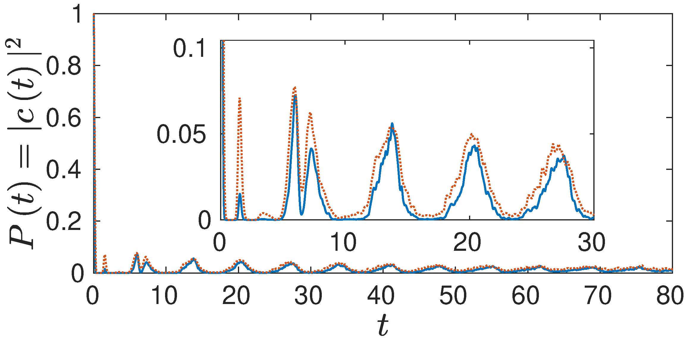
In Figure 1, we compare the full numerical solution to the time-dependent Schrödinger equation (TDSE) with the corresponding semiclassical HK result. It can be seen that the two results coincide very nicely, although the HK result due to the loss of norm is not coming back to unity fully at the revival time, which is around $t=75$. The fact that the semiclassical HK propagator can reproduce the interference based revival in a Morse oscillator has been investigated in detail by Wang and Heller [30].

In Figure 2, we compare several LSC-IVR results. The Wigner and Husimi results differ as well as does the Husimi without the additional exponential term. For short times all three results are identical. For times when all three results have decayed to small values, differences become visible. The new Husimi and the Wigner result are very close, though. The revival visible in the full quantum result is not displayed in any of the linearized approaches, though.

4.2. Coupling to a Harmonic Bath Degree of Freedom

Now we proceed and ask the question what happens to the revival dynamics, if we couple the Morse oscillator to a very heavy harmonic oscillator of mass $m_y=20$ such that the total Hamiltonian reads

$$\begin{array}{c}\hfill H=\frac{p_x^2}{2}+\frac{p_y^2}{2m_y}+V_M\left(x\right)+\frac{1}{2}{m}_y{\omega }_y^2{y}^2+\lambda xy,\end{array}$$

(77)

with ${\omega }_y=1.17$ and the initial width parameter for the ground state wavepacket in the harmonic degree ${\gamma }_y=m_y{\omega }_y$. The very heavy oscillator shall mimic the interaction with a many degree of freedom bath with smaller masses, i.e., a “condensed phase” environment, see also [15].

First, we look at a moderate coupling strength of $\lambda =1$. The corresponding results from the Wigner and the Husimi approach as well as the Husimi without the $\frac{{\mathbf{b}}^{\mathrm{T}}{\mathbf{A}}^{-1}\mathbf{b}}{4}$ term in the exponent are contrasted in Figure 3. It can be seen that the additional term brings the Husimi result closer to the Wigner one, rather similar to the uncoupled case. At longer times there is just a small amplitude wiggling in the signal due to the coupling.

In Figure 4, we turn to a higher coupling strength of $\lambda =9$ and first compare the full solution to the TDSE with the corresponding semiclassical HK result. It can be seen that, as in the uncoupled case, the two results again coincide very nicely, even the small oscillations are reproduced until around $t=75$. The revival is not visible any more, due to the strong coupling to the harmonic degree, however.

In Figure 5, the results from the LSC-IVR calculations (Wigner as well as Husimi) in the strong coupling case are displayed. It can be seen that both also show no revivals, as to be expected. For the very strong coupling the underlying classical dynamics becomes strongly chaotic and the numerical inversion of the $\mathbf{A}$ matrix turns singular at certain times for a lot of the 10,000 trajectories we propagated. In order to circumvent this singularity problem, we treated the problematic trajectories without the additional term in the exponent from the time on, when the inversion is problematic.

5. Conclusions and Outlook

The aim of this presentation was two-fold. The first goal was to highlight that the Wigner-Weyl and Husimi transform version of linearized semiclassical theories can lead to the same final formula, whereas they are quite different in the case of the survival probability, where strictly, the simple Husimi version is not applicable. This fact then established a second goal: to find the correct Husimi-like version of the linearized semiclassical IVR. This goal was achieved by straightforward linearization of the double HK expression for the survival (or staying) probability. In the course of the derivation we also slightly generalized a seminal calculation by Herman (see the appendix of [28]) to the case of width parameter matrices that are not proportional to the unit matrix.

The newly developed formalism was then applied to the revival dynamics in a Morse oscillator. The revival, being a quantum interference phenomenon, could, apart from the numerically converged full quantum results, only be observed in the full HK results, however. Both LSC-IVR variants show a monotonically decaying envelope and no revival. Coupling the Morse oscillator to a heavy bath oscillator leads to the absence of the revival in the full quantum calculations also. In this case the LSC-IVR results are predicting the correct behavior to a large degree and full quantum calculations are not necessary, the system dynamics has undergone a quantum to classical transition due to the coupling to the environment, similar to the findings predicted using the semiclassical hybrid dynamics [20].

For the future, it might be worthwhile to look at even more general correlations function, the so-called out of time order correlators [31] in the (linearized) semiclassical IVR approach.