Uniform Hyperbolicity of a Scattering Map with Lorentzian Potential

Abstract

We show that a two-dimensional area-preserving map with Lorentzian potential is a topological horseshoe and uniformly hyperbolic in a certain parameter region. In particular, we closely examine the so-called sector condition, which is known to be a sufficient condition leading to the uniformly hyperbolicity of the system. The map will be suitable for testing the fractal Weyl law as it is ideally chaotic yet free from any discontinuities which necessarily invokes a serious effect in quantum mechanics such as diffraction or nonclassical effects. In addition, the map satisfies a reasonable physical boundary condition at infinity, thus it can be a good model describing the ionization process of atoms and molecules.

1. Introduction

The periodically kicked one-degree-of-freedom system has been playing and still plays significant roles in the study of chaos in classical and quantum systems. The discovery of quantum suppression of classical chaos was made by properly formulating quantum mechanics of the classical kicked system [1], and then it invoked an unexpected formal link between the eigenfunction equation of the kicked system and the Anderson model in the condensed matter field [2]. The kicked system has been further applied to explore experimental manifestations of chaos in atomic and molecular systems, especially ionization of the hydrogen atom in an external electronic field [3]. It was actually realized based the optical lattice in the cold atom system [4].

A great advantage of the kicked system is that one can easily design the classical phase space and realize various types of phase space ranging from completely integrable to mixed ones by choosing potential functions appropriately. The most often used version would be the so-called Chirikov–Taylor standard map, for which signatures of classical dynamics have been extensively studied [5,6]. It is well known that when the kicking strength is small enough Kolmogorov–Arnold–Moser (KAM) curves predominate the phase space, and the motion around KAM curves becomes sticky. After the breakdown of KAM curves, Poincaré Birkhoff chains and cantori appear as well and the topology of phase space becomes enormously complex in general.

As the kicking strength gets large, those regular components, remnants of complete integrability, gradually disappear. It is eventually observed that the phase space is almost covered by chaotic orbits. However, even after considerable efforts were made, rigorous results on the signature of generic situations are limited and it is not yet clear whether or not the system becomes ideally chaotic, more precisely uniformly hyperbolic when the kicking strength is large enough. Although it is possible to prove the existence of “chaotic orbits” in a large but finite kicking strength region [7], meaning that the orbits which are conjugate to symbolic dynamics defined in the infinity limit of the kicking strength survive, it does not necessarily mean that all the orbits are chaotic. Therefore the standard map is particularly suitable for studying the KAM scenario, the transition from completely integrable (zero kicking strength) to mixed dynamics, thus has been taken as a good toy model realizing mixed phase space, but the connection to ideally chaotic situations is not yet obvious.

On the other hand, there exist maps for which ideally chaotic situations are actually realized. A certain class of area-preserving the maps defined on the torus ${\mathbb{T}}^2$, the so-called torus automorphism, satisfies the uniform hyperbolicity. A well known example is the Arnold cat map, and it keeps uniform hyperbolicity because of the structural stability [8]. Another paradigm achieving uniform hyperbolicity is the map defined on the plane ${\mathbb{R}}^2$ and the most standard and extensively studied one is the Hénon family. The Hénon map is known to be the simplest polynomial diffeomorphism exhibiting chaos. This fact owes to the classification theorem of Friedland and Milnor [9]. In a certain parameter regime, the horseshoe is realized and the uniform hyperbolidity was proved to hold [10], and later it has been shown to be true until when the first tangency between stable and unstable manifolds happens [11].

Such systems are better suited to examine classical and quantum signatures of ideally chaotic situations and been often taken to be toy models for such a purpose. However, as torus automorphisms with uniform hyperbolicity do not have an integrable limit in their parameter spaces, so the connection to the KAM scenario is not clear enough. As for the area-preserving Hénon map, the behavior around infinity is somewhat unphysical because the potential function is given as a cubic function. Therefore, once orbits are scattered from a scattering region, they are accelerated and diverges superexponentially to infinity. A complete ideal horseshoe can be formed in the Hénon map but the boundary condition would be physically improper.

It is, therefore, desirable to find a map which has a natural integrable limit, possibly achieved by taking the zero kicking strength limit, and at the same time can become uniformly hyperbolic over a certain parameter space, yet satisfying a physically feasible boundary condition. In this paper, we show that a scattering map whose potential shape is given by the Lorentzian function has a parameter region, in which it meets such requirements. Herein, we use an essentially the same technique applied to the map with another types of potentials including the Gaussian function [12], but some details depend on the specific form of potential functions.

We remark that there is a strong motivation to seek a uniformly hyperbolic scattering map with analytic potential. As argued in [12], if the map contains a discontinuity, it necessarily invokes a serious effect in the corresponding quantum mechanics such as diffraction or nonclassical effects. As a result, if one performs a test to verify the so-called fractal Weyl law, which concerns the crudest quantum-to-classical correspondence in scattering systems, and a counterpart of the Weyl law in the bounded system, such nonclassical effects are difficult to be handled and should better be avoided because it makes it difficult to develop semiclassical arguments. The fractal Weyl law claims that the number of long-lived resonance states should grow as a power law whose exponent is related to the fractal dimension of the classical repeller [13]. As was illustrated in [12] that projective openings or strong absorbing potentials make the separation of resonance eigenvalues from the continuum almost impossible, which raises a doubt that the obtained spectra are well-qualified for the purpose. For this very reason, uniformly hyperbolic scattering maps with analytic potential are strongly sought.

The outline of the paper is as follows. In Section 2, we provide the scattering map analyzed in this paper, and show numerical evidence suggesting that the map can be a topological horseshoe and uniformly hyperbolic. In Section 3, we first present some pieces of numerical evidence illustrating that the map exhibits the horseshoe if the perturbation strength is large enough, and then provide a sufficient condition leading to the topological horseshoe. In Section 4, we show that the system has a filtration property, meaning that the non-wandering set of the system is confined in a certain finite domain. In Section 5, we present a sufficient condition for the system to be uniformly hyperbolic. We here apply the sector condition, which is known to be a sufficient for uniform hyperbolicity, in order to check the uniform hyperbolicity of the system. In Section 6, we closely examine under which conditions the sector condition holds. In Section 7, we make a comment on the optimality of our estimate and also mention a possible generalization.

2. Scattering Map

The Hamiltonian of the periodically kicked one-degree-of-freedom system is given by

$$\begin{array}{c}\hfill H(q,p;t)=\frac{p^2}{2}+V\left(q\right)\sum _{n\in \mathbb{Z}}\delta (t-n),\end{array}$$

(1)

where $V\left(q\right)$ is a potential function controlling the dynamics. Here, unlike the standard map or similar types of maps defined on cylindrical or toric phase space, we consider the map defined on the plane ${\mathbb{R}}^2$, which provides scattering dynamics in general.

Since we want to set a physically feasible scattering system, the kicking potential $V\left(q\right)$ should tend to zero sufficiently fast as $\left|q\right|$ goes to infinity,

$$\begin{array}{c}\hfill \underset{q\to \pm \infty }{lim}V\left(q\right)=0,\end{array}$$

(2)

resulting in the free motion in the asymptotic region. A simple choice meeting such a condition would be to take the Gaussian as a potential function. In the attractive Gaussian case, Jensen indeed used it to investigate quantum effects on scattering processes [14,15], and the system can be experimentally approximated by a Gaussian laser beam action of cold atoms. Fishman and coworkers have also studied classical and quantum aspects in mixed regime have also been studied [16]. The repulsive Gaussian case has been also used to study quantum tunneling effects in terms of complex semiclassical theory [17,18].

The classical dynamics of periodically kicked systems can be reduced to discrete dynamics via stroboscopic phase-space section. They are obtained by integrating Hamilton’s equations of motion over one period in time. Following the work in [12], we here adopt a two-dimensional area-preserving map in a symmetrized version:

$$\begin{array}{c}\hfill U:\left(\begin{array}{c}{q}_{n+1}\\ p_{n+1}\end{array}\right)=\left(\begin{array}{c}{\displaystyle q_n+p_n-\frac{1}{2}{V}^{\prime }\left(q_n\right)}\\ {\displaystyle p_n-\frac{1}{2}{V}^{\prime }\left(q_n\right)-\frac{1}{2}{V}^{\prime }\left(q_{n+1}\right)}\end{array}\right).\end{array}$$

(3)

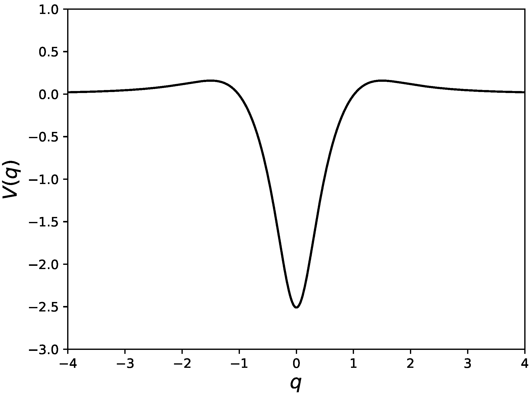
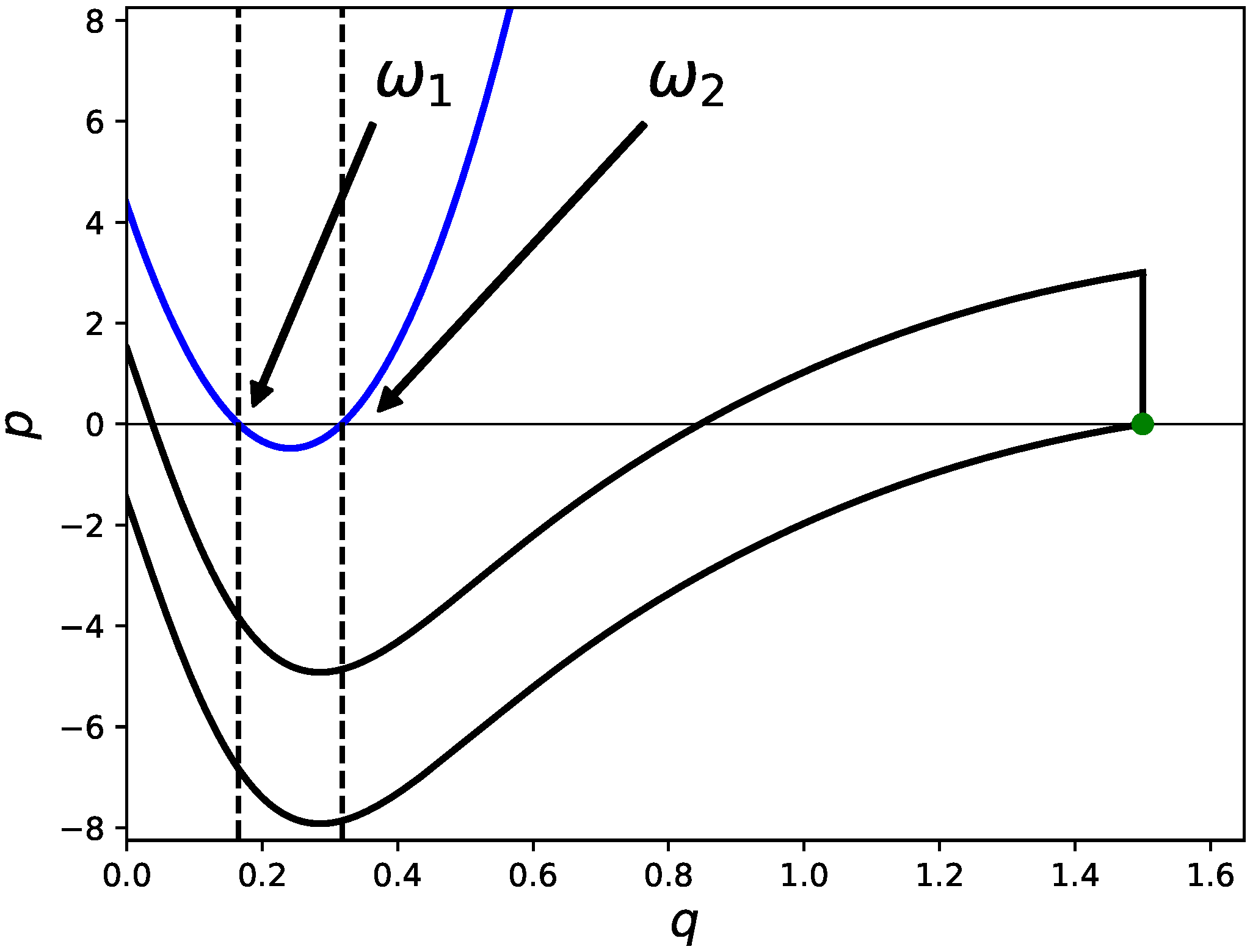
Here, we take the potential function (also see Figure 1),

$$\begin{array}{c}\hfill V\left(q\right)=-\kappa \left\{f_1\left(q\right)-\epsilon \left(f_2(q-q_b)+f_2(q+q_b)\right)\right\},\end{array}$$

(4)

with Lorentzian functions

$$\begin{array}{c}\hfill f_1\left(q\right)=\frac{1}{1+4q^2},\end{array}$$

(5)

$$\begin{array}{c}\hfill f_2\left(q\right)=\frac{1}{1+q^2}.\end{array}$$

(6)

In the following, $\kappa >0$ is assumed, and the parameter $\epsilon$ is expressed in terms of other parameters $q_b$ and $q_f$ as

$$\begin{array}{c}\hfill \epsilon =\frac{f_1^{\prime }\left(q_f\right)}{f_2^{\prime }(q_f-q_b)+f_2^{\prime }(q_f+q_b)}.\end{array}$$

(7)

The parameter $q_b$ represents the amount of the shift of two superposed potential functions $f_1\left(q\right)$ and $f_2\left(q\right)$, and $\pm q_f$ denote the positions where the potential function $V\left(q\right)$ takes extremum values, i.e.,

$$\begin{array}{c}\hfill V^{\prime }\left(q_f\right)=-\kappa \left\{f_1^{\prime }\left(q_f\right)-ϵ\left(f_2^{\prime }(q_f-q_b)+f_2^{\prime }(q_f-q_b)\right)\right\}=0.\end{array}$$

The potential function $V\left(q\right)$ is thus specified by three parameters: $\kappa ,q_b$, and $q_f$.

Throughout the following argument we fix

$$\begin{array}{c}\hfill q_b=1.0, q_f=1.5,\end{array}$$

(8)

which leads to

$$\begin{array}{c}\hfill \epsilon \approx 0.1632\cdots .\end{array}$$

(9)

We will explore the region for $\kappa$, in which the system is a topological horseshoe and uniformly hyperbolic as well. As will be mentioned in the concluding section, it would be desirable to investigate the whole parameter space including $q_b$ and $q_f$, and numerical observations show the existence of parameter regions, in which the horseshoe and hyperbolicity are realized in wider range of $(q_b,q_f)$ including the one specified above. Therefore, although we fix the parameters $q_b$ and $q_f$ in the subsequent analysis, it does not necessarily mean that the horseshoe and hyperbolicity would not be achieved at other parameter values. 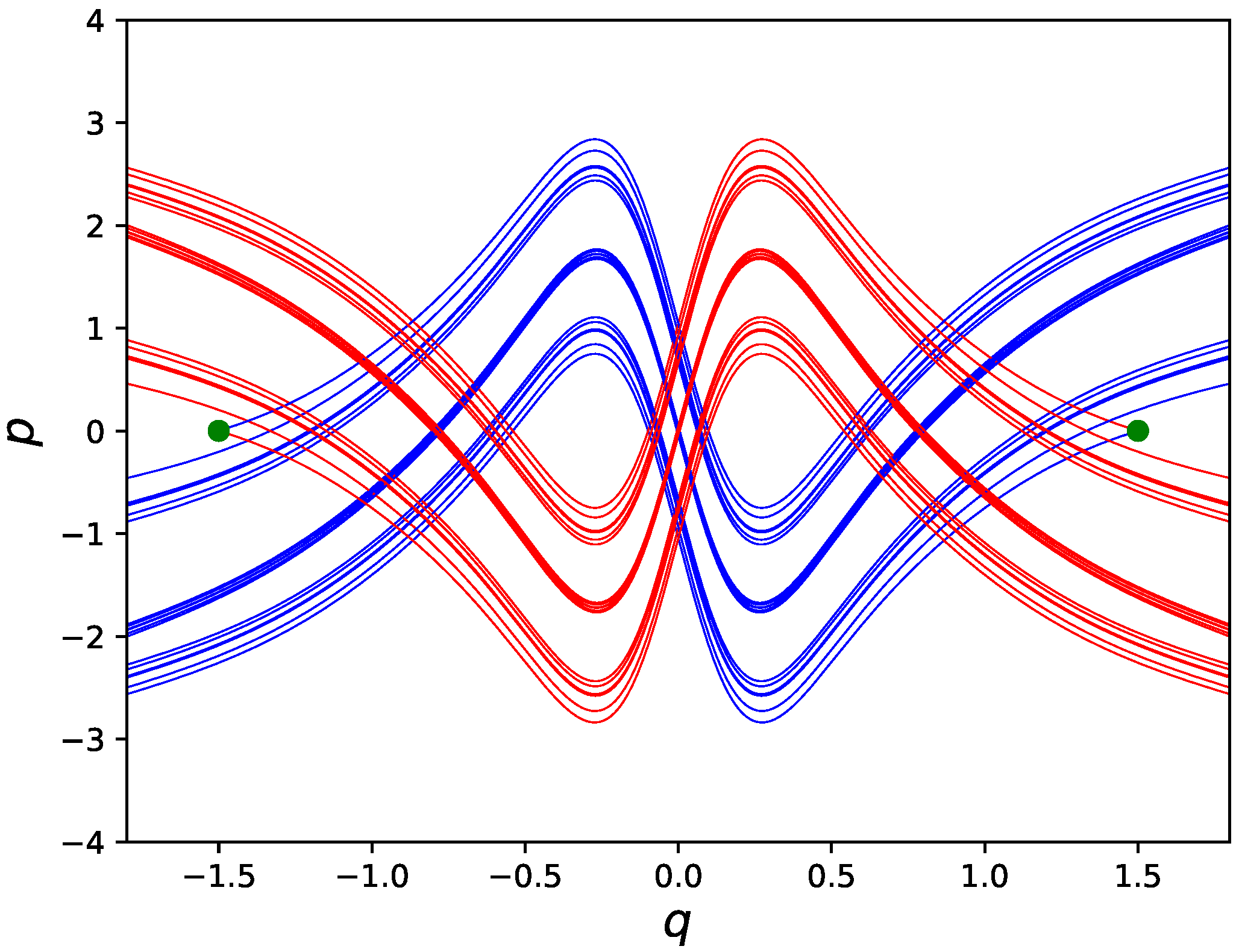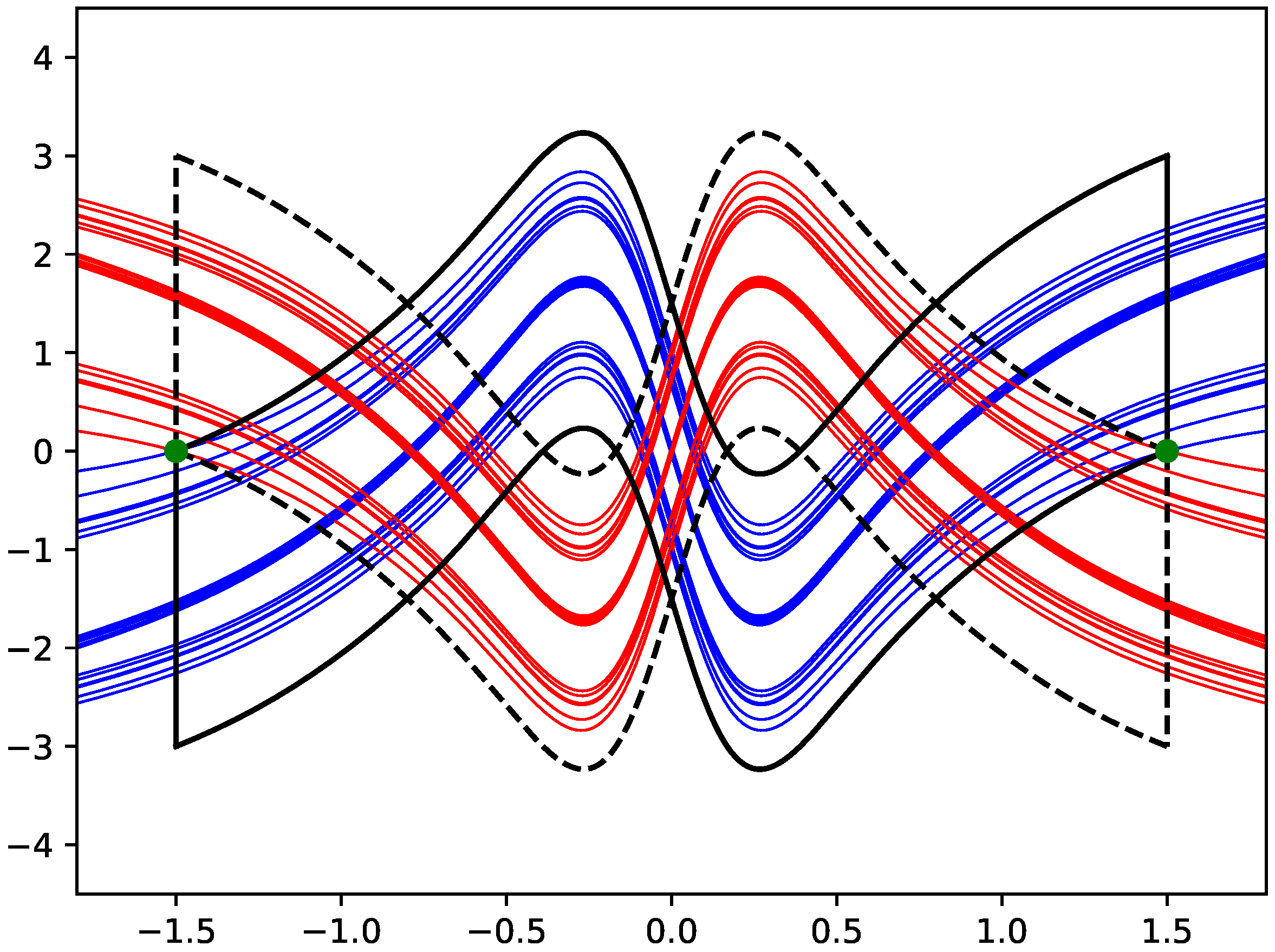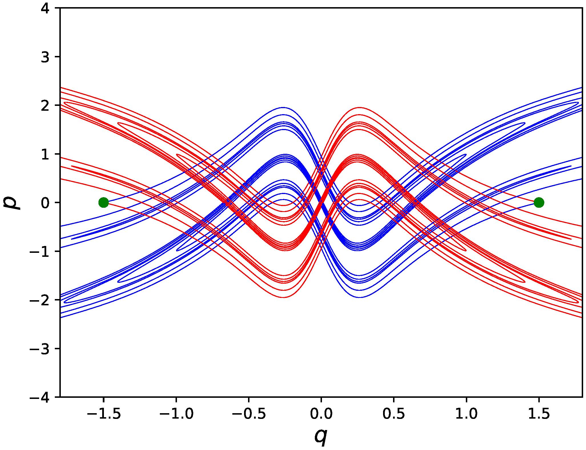However, it is too elaborate to develop analytical arguments and provide a rigorous proof for the case including the $q_b$ and $q_f$, so we here concentrate on a specific parameter set. Stable and unstable manifolds for $q_b=1.0$ and $q_f=1.5$ are illustrated in Figure 2.

3. Horseshoe Condition

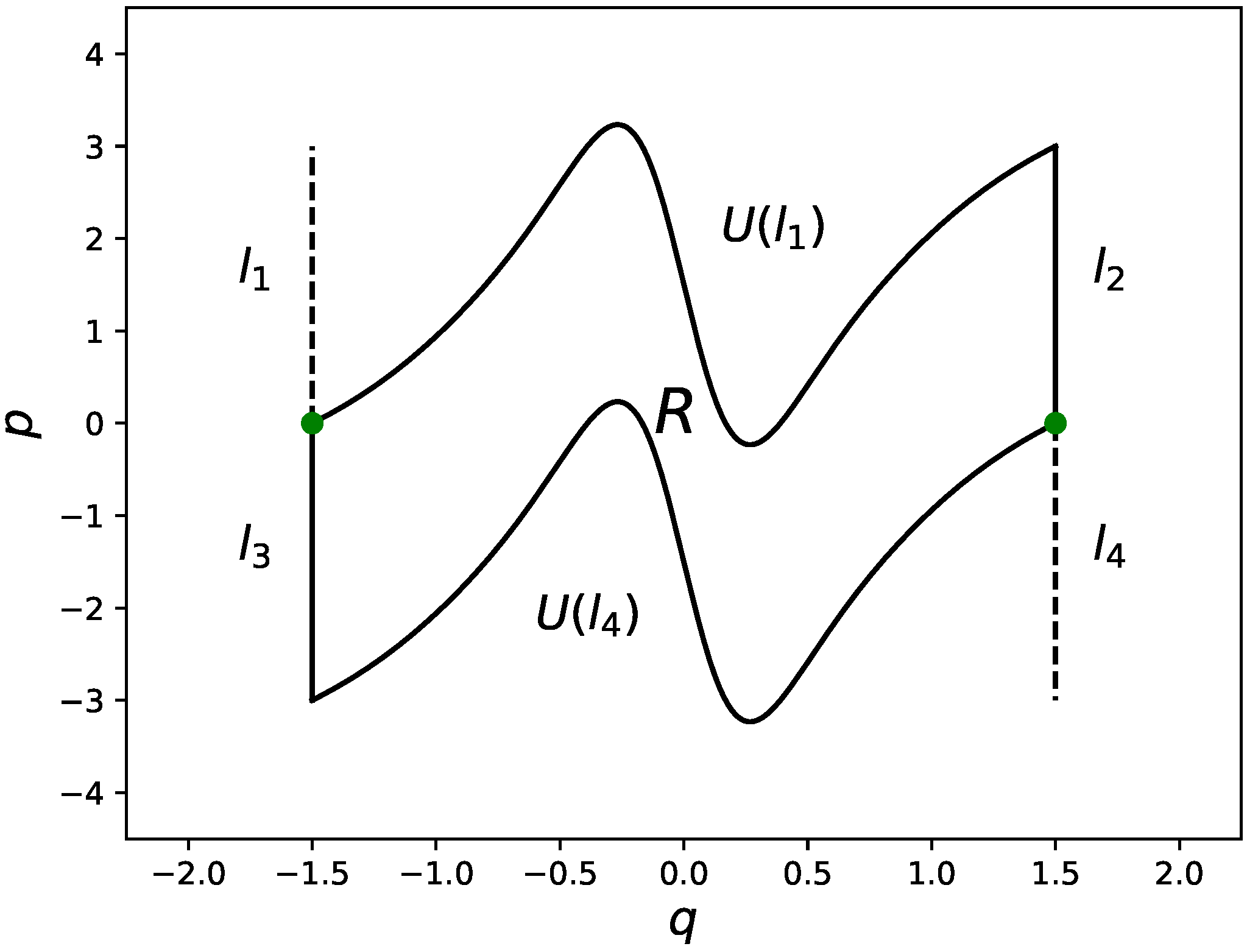
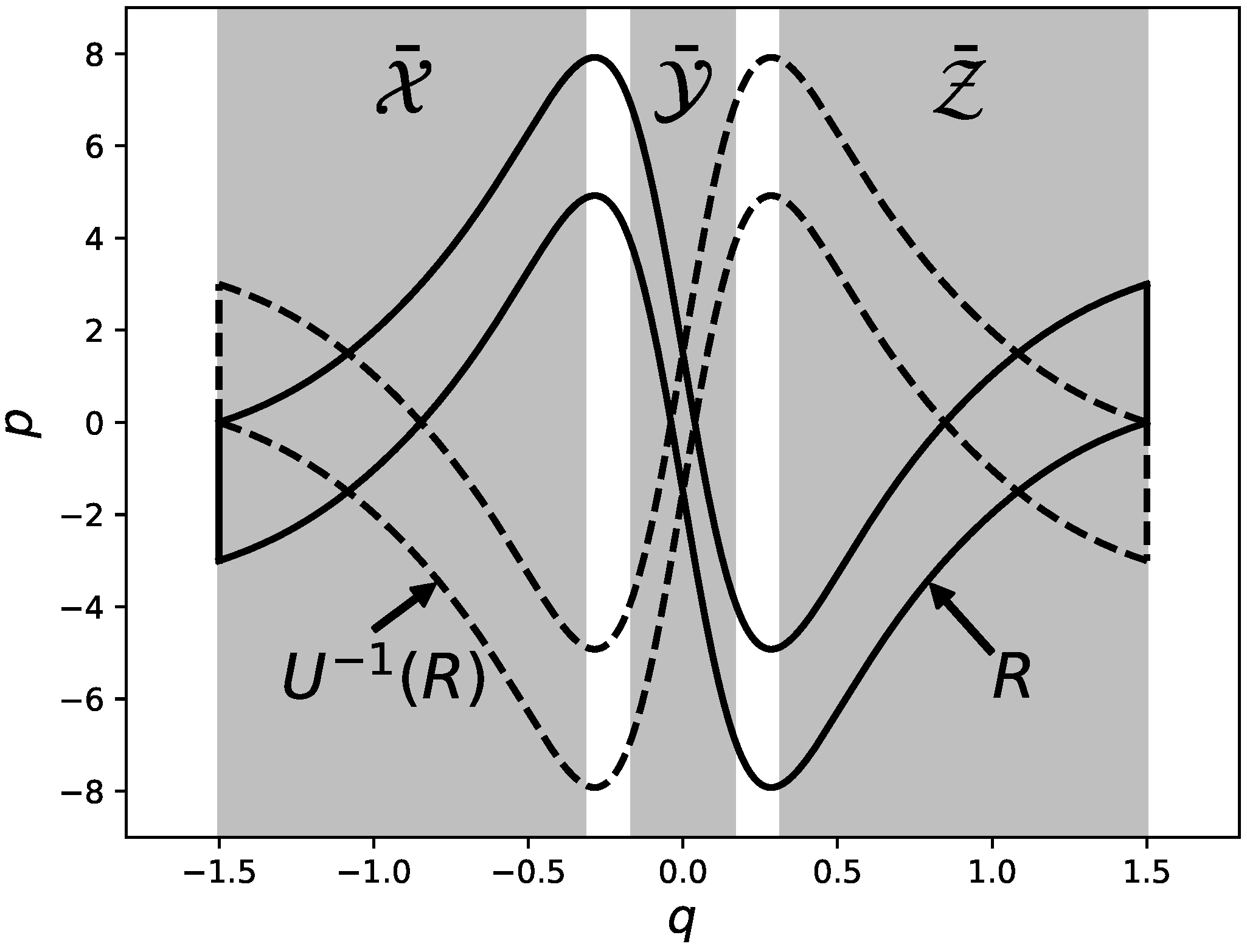
In this section, we will show that the map (3) can be a topological horseshoe in a certain parameter region. To this end, let us consider the following four line segments:

$$\begin{array}{ccc}\hfill l_1& :=& \left\{(q,p)\right|q=-q_f,0<p<2q_f\},\hfill \end{array}$$

(10)

$$\begin{array}{ccc}\hfill l_2& :=& \left\{(q,p)\right|q=q_f,0<p<2q_f\},\hfill \end{array}$$

(11)

$$\begin{array}{ccc}\hfill l_3& :=& \left\{(q,p)\right|q=-q_f,-2q_f<p<0\},\hfill \end{array}$$

(12)

$$\begin{array}{ccc}\hfill l_4& :=& \left\{(q,p)\right|q=q_f,-2q_f<p<0\},\hfill \end{array}$$

(13)

and introduce the region R, whose boundaries are formed by the curves $l_2,l_3,U\left(l_1\right)$ and $U\left(l_4\right)$. The inverse image of R is enclosed by the curves $l_1,l_4,U^{-1}\left(l_2\right)$ and $U^{-1}\left(l_3\right)$ (see Figure 3). The boundary curves for R and $U^{-1}\left(R\right)$ are expressed as

$$\begin{array}{c}U\left(l_1\right):=\left\{(q,p)\right|-q_f<q<q_f,p=F\left(q\right)\},\hfill \end{array}$$

(14)

$$\begin{array}{c}{U}^{-1}\left(l_2\right):=\left\{(q,p)\right|-q_f<q<q_f,p=-F\left(q\right)+2q_f\},\hfill \end{array}$$

(15)

$$\begin{array}{c}{U}^{-1}\left(l_3\right):=\left\{(q,p)\right|-q_f<q<q_f,p=-F\left(q\right)\},\hfill \end{array}$$

(16)

$$\begin{array}{c}U\left(l_4\right):=\left\{(q,p)\right|-q_f<q<q_f,p=F\left(q\right)-2q_f\},\hfill \end{array}$$

(17)

where

$$\begin{array}{ccc}\hfill F\left(q\right)& =& q+q_f-\frac{1}{2}{V}^{\prime }\left(q\right)\hfill \\ \hfill & =& q+q_f-\kappa \left\{\frac{4q}{{(1+4q^2)}^2}-\epsilon \left(\frac{q-q_b}{{(1+{(q-q_b)}^2)}^2}+\frac{q+q_b}{{(1+{(q+q_b)}^2)}^2}\right)\right\}.\hfill \end{array}$$

(18)

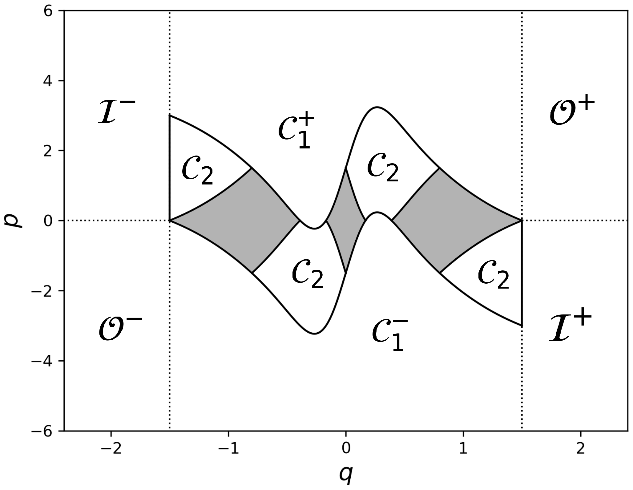
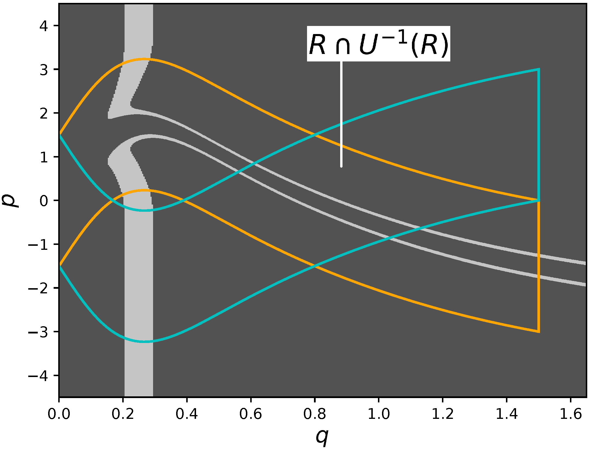
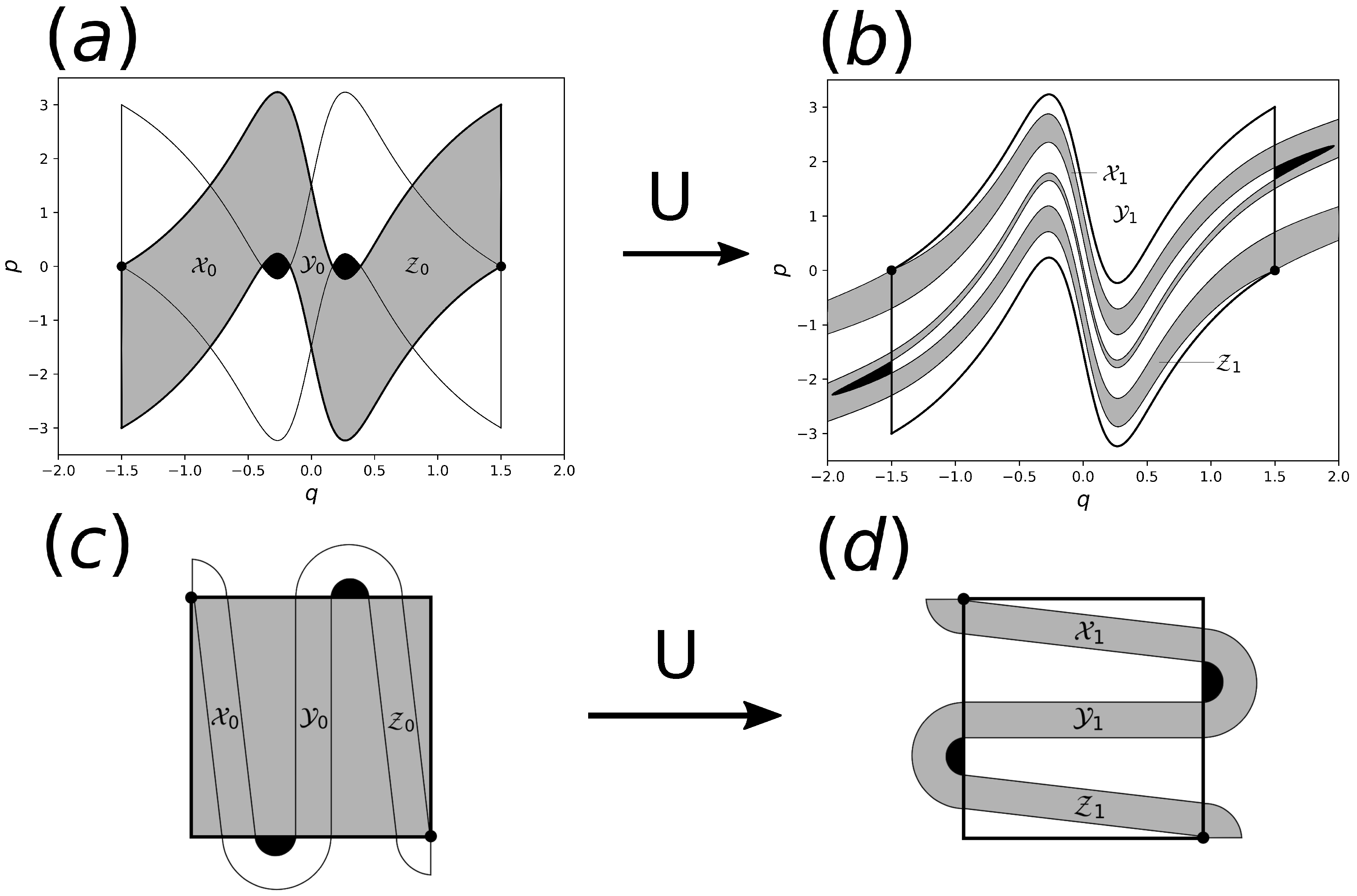
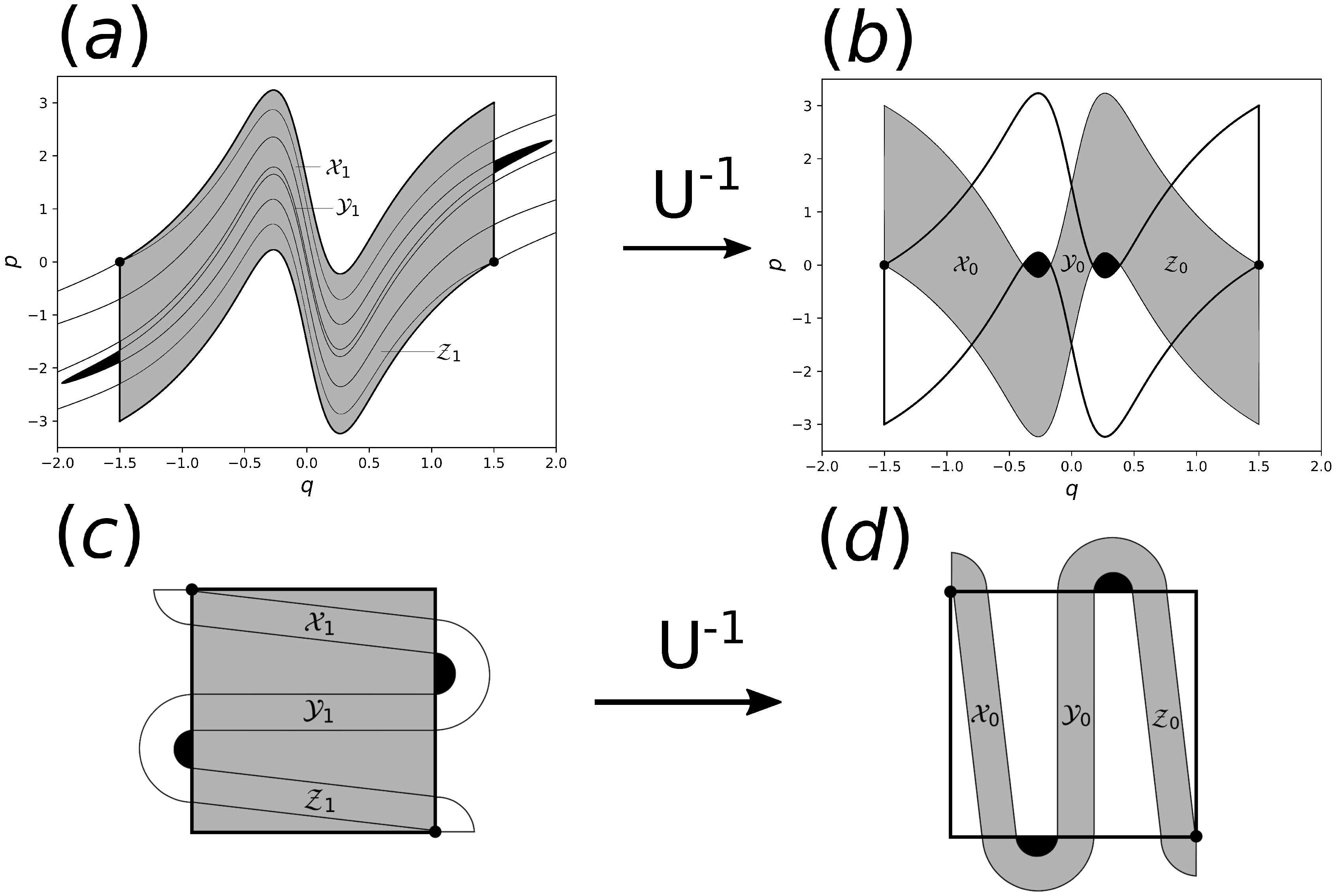
For the region R introduced above, if $\kappa$ is sufficiently large, the numerical observation reveals that the intersection between R and its forward iteration $U\left(R\right)$ is composed of three disjointed regions:

$$\begin{array}{c}\hfill R\cap U\left(R\right)={\mathcal{X}}_1\cup {\mathcal{Y}}_1\cup {\mathcal{Z}}_1,\end{array}$$

(19)

where

$$\begin{array}{c}\hfill {\mathcal{X}}_1\cap {\mathcal{Y}}_1=\varnothing ,{\mathcal{Y}}_1\cap {\mathcal{Z}}_1=\varnothing ,{\mathcal{Z}}_1\cap {\mathcal{X}}_1=\varnothing ,\end{array}$$

(20)

In a similar way, the backward iteration yields

$$\begin{array}{c}\hfill R\cap U^{-1}\left(R\right)={\mathcal{X}}_0\cup {\mathcal{Y}}_0\cup {\mathcal{Z}}_0.\end{array}$$

(21)

where

$$\begin{array}{c}\hfill {\mathcal{X}}_0\cap {\mathcal{Y}}_0=\varnothing ,{\mathcal{Y}}_0\cap {\mathcal{Z}}_0=\varnothing ,{\mathcal{Z}}_0\cap {\mathcal{X}}_0=\varnothing .\end{array}$$

(22)

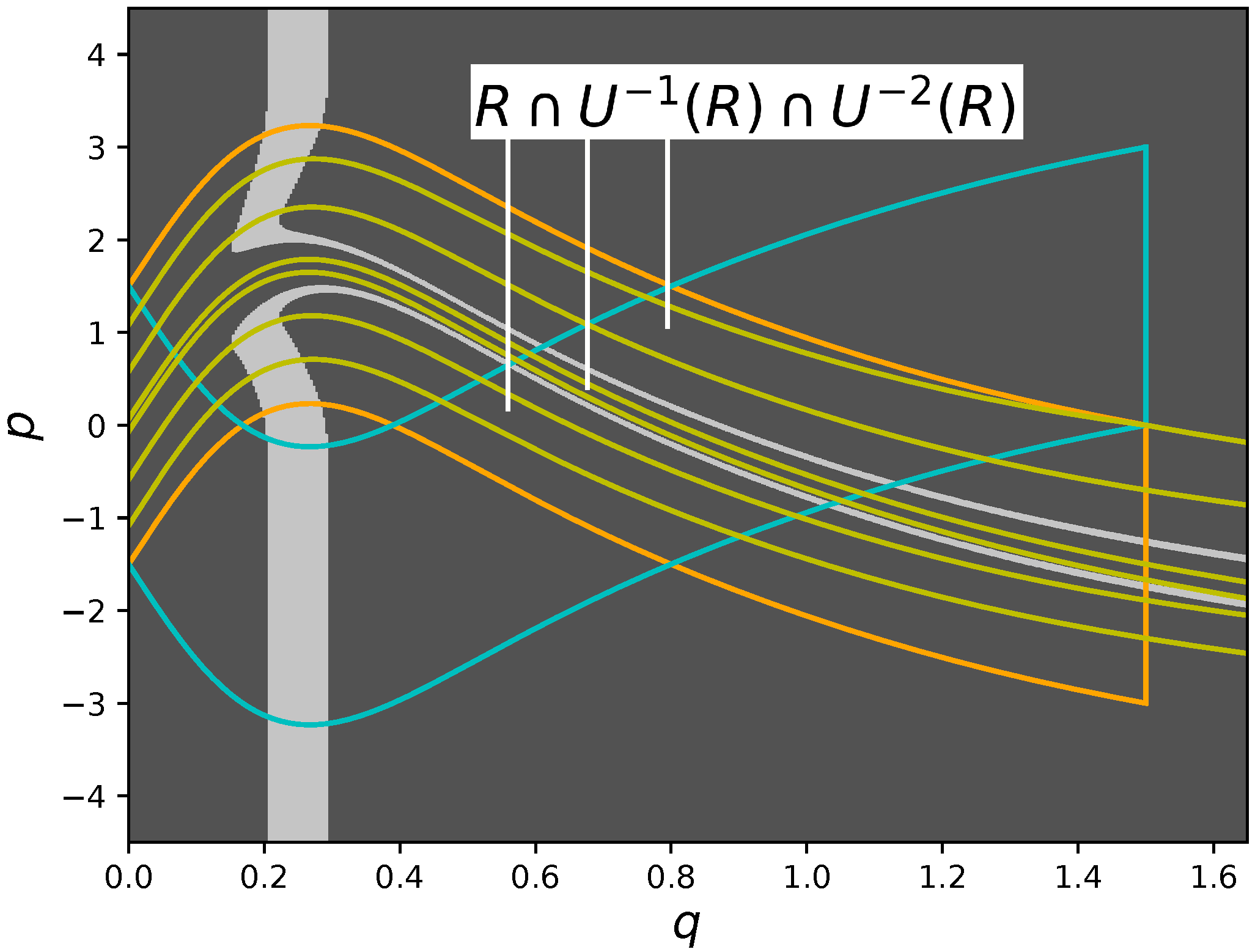
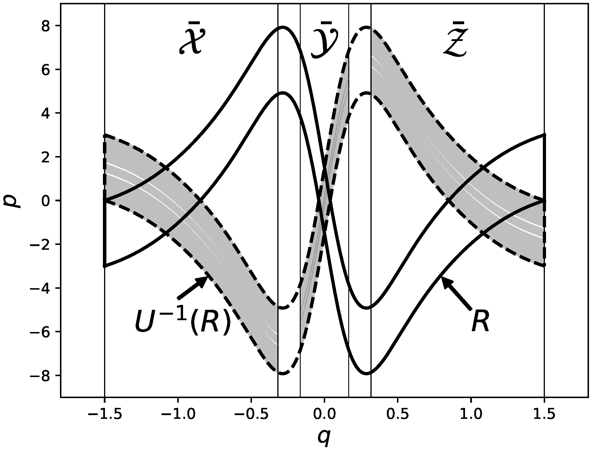
As displayed in Figure 4 and Figure 5, the twice-folded horseshoe is created under the iteration, unlike the standard once-folded one, and hence the existence of the black region in the figures could be a sufficient condition for the horseshoe.

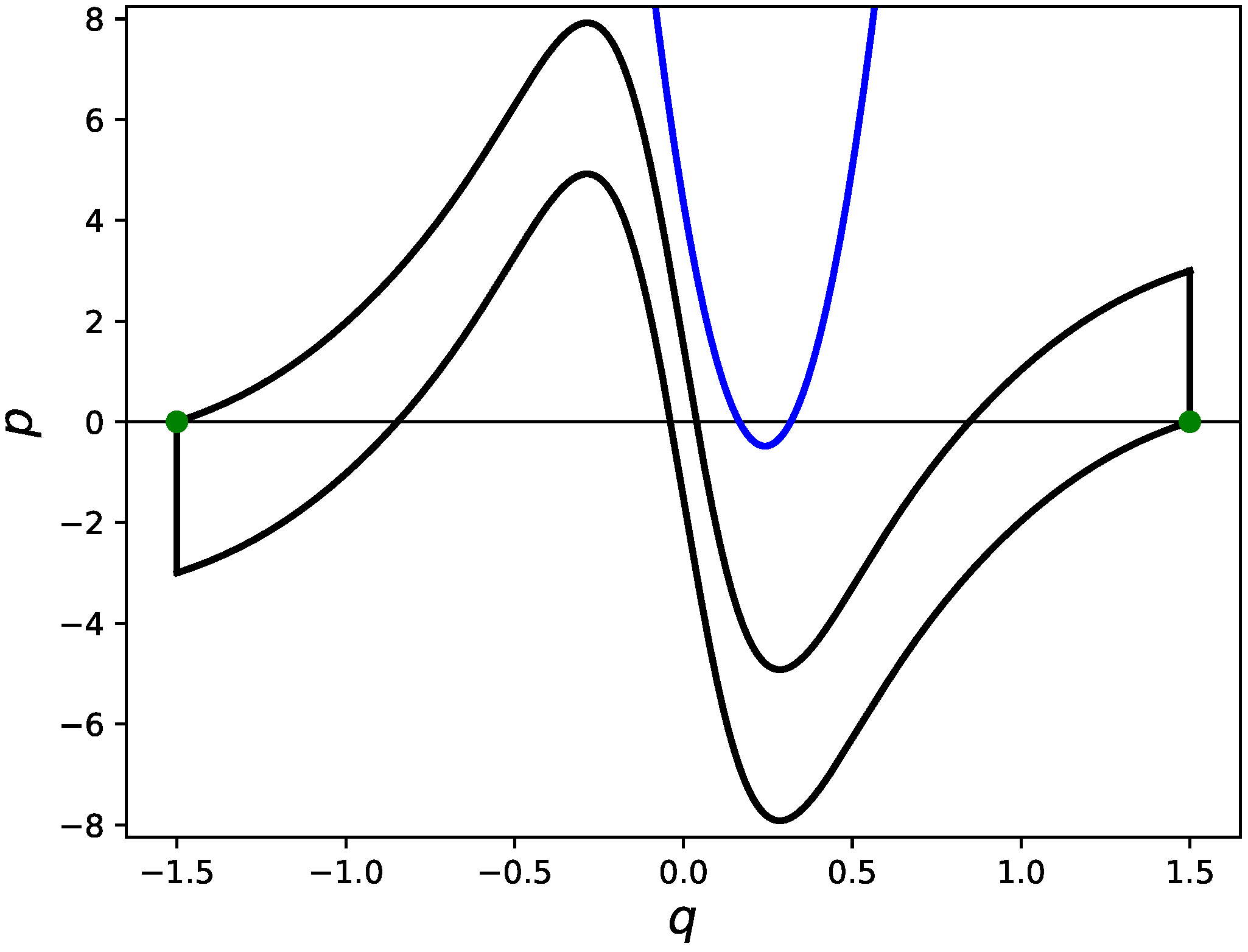
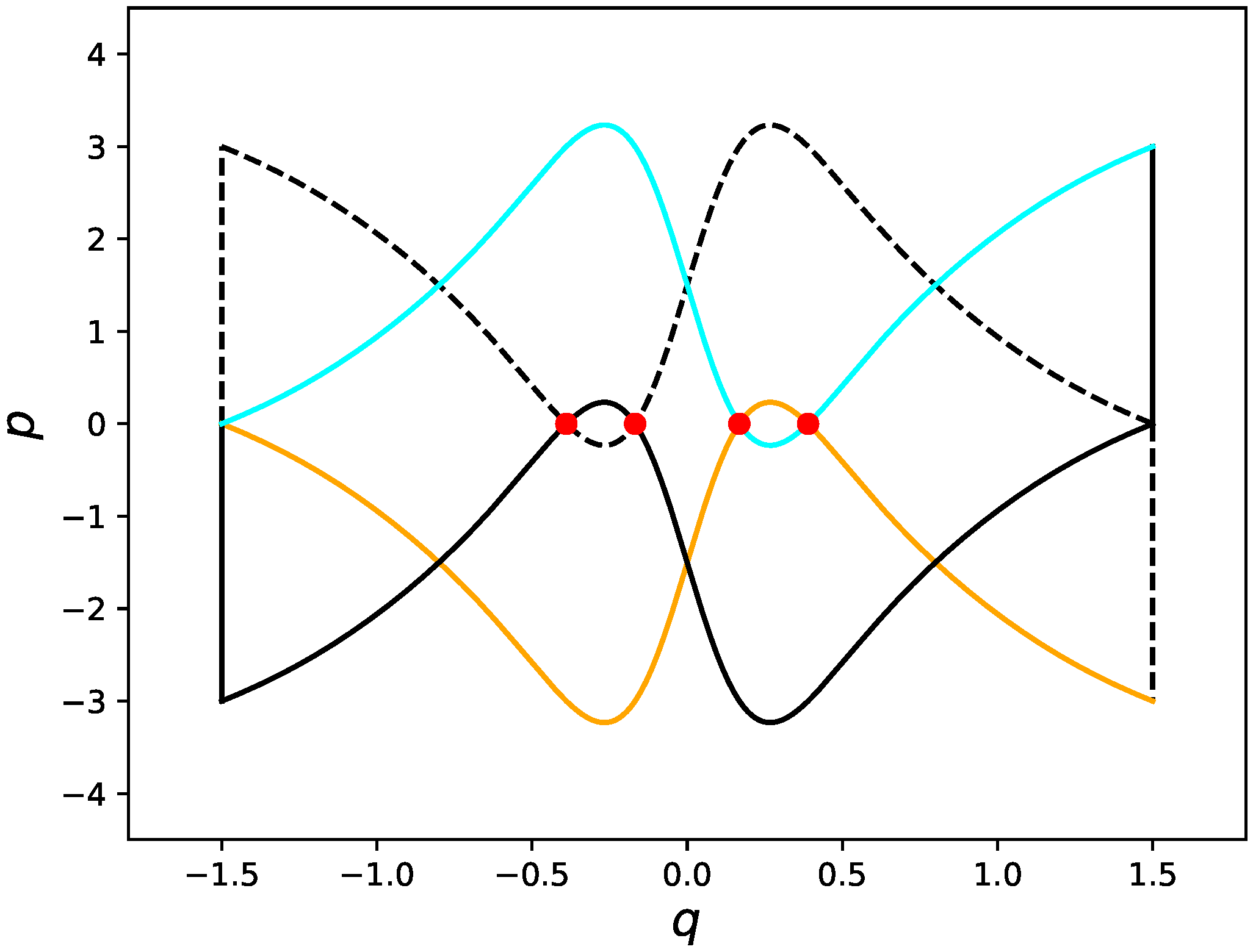
As shown in Figure 6, if $U\left(l_1\right)$ and $U^{-1}\left(l_3\right)$ intersect transversally at two points in the interval $0<q<q_f$, the horseshoe is realized. If such a situation happens, it is needless to say that $U\left(l_4\right)$ and $U^{-1}\left(l_2\right)$ intersect transversally in the interval $-q_f<q<0$ as well. Because of the symmetry with respect to the q-axis, one can say that this situation is equivalently achieved if the curve $U\left(l_1\right)$ intersects the q-axis transversally at two distinct points in the interval $0<q<q_f$. Since $F\left(0\right)=q_f>0,F\left(q_f\right)=2q_f>0$, if

$$\begin{array}{c}\hfill \underset{0<q<q_f}{min}F\left(q\right)<0,\end{array}$$

(23)

is satisfied, then $U\left(l_1\right)$ and $U^{-1}\left(l_3\right)$, $U\left(l_4\right)$ and $U^{-1}\left(l_2\right)$ as well, have intersections, yielding the shaded regions as illustrated in Figure 4, which results in a topological horseshoe. As a sufficient condition to bring such a situation, we obtain the following.

Proposition 1.

If κ satisfies the condition

$$\begin{array}{c}\hfill \kappa \ge \frac{{\displaystyle 2q_f}}{{\displaystyle \frac{3\sqrt{3}}{8}-c_1\epsilon }},\end{array}$$

(24)

then${\displaystyle \Lambda =\bigcap _{n\in \mathbb{Z}}{U}^n\left(R\right)}$is a topological horseshoe.

Proof. 

First note that the function $(q-q_b)/{(1+{(q-q_b)}^2)}^2$ takes the maximum value $3\sqrt{3}/16$ at $q=q_b+1/\sqrt{3}$, and the minimum value $-3\sqrt{3}/16$ at $q=q_b-1/\sqrt{3}$. As $q_b>1/\sqrt{3}$, the function $(q+q_b)/{(1+{(q+q_b)}^2)}^2$ monotonically decreases for $q>0$. In addition, $(q+q_b)/{(1+{(q+q_b)}^2)}^2<q_b/{(1+q_b^2)}^2$ holds, which leads to an upper bound for $F\left(q\right)$

$$\begin{array}{c}\hfill F\left(q\right)<2q_f-\kappa \frac{4q}{{(1+4q^2)}^2}+\kappa \epsilon \left(\frac{3\sqrt{3}}{16}+\frac{q_b}{1+q_b^2}\right).\end{array}$$

(25)

Similarly, the function $-4q/{(1+4q^2)}^2$ takes the minimum value $q=1/2\sqrt{3}$ at $q=1/2\sqrt{3}$ and this also attains the minimum value for $0<q<q_f$ since $1/2\sqrt{3}<q_f$. Then, we have

$$\begin{array}{c}\hfill \underset{0<q<q_f}{min}F\left(q\right)<2q_f-\frac{3\sqrt{3}}{8}\kappa +\kappa \epsilon c_1.\end{array}$$

(26)

Here, $c_1$ denotes a constant

$$\begin{array}{c}\hfill c_1:=\left(\frac{3\sqrt{3}}{16}+\frac{q_b}{1+q_b^2}\right).\end{array}$$

(27)

Therefore, as a sufficient condition for

$$\begin{array}{c}\hfill \underset{0<q<q_f}{min}F\left(q\right)<0,\end{array}$$

(28)

we obtain the inequality

$$\begin{array}{c}\hfill 2q_f-\frac{3\sqrt{3}}{8}\kappa +\kappa \epsilon c_1\le 0.\end{array}$$

(29)

By explicitly evaluating

$$\begin{array}{c}\hfill \epsilon \approx 0.1632\cdots <\frac{3\sqrt{3}}{8c_1}\approx 1.1300\cdots ,\end{array}$$

(30)

we reach the desired inequality (24) □.

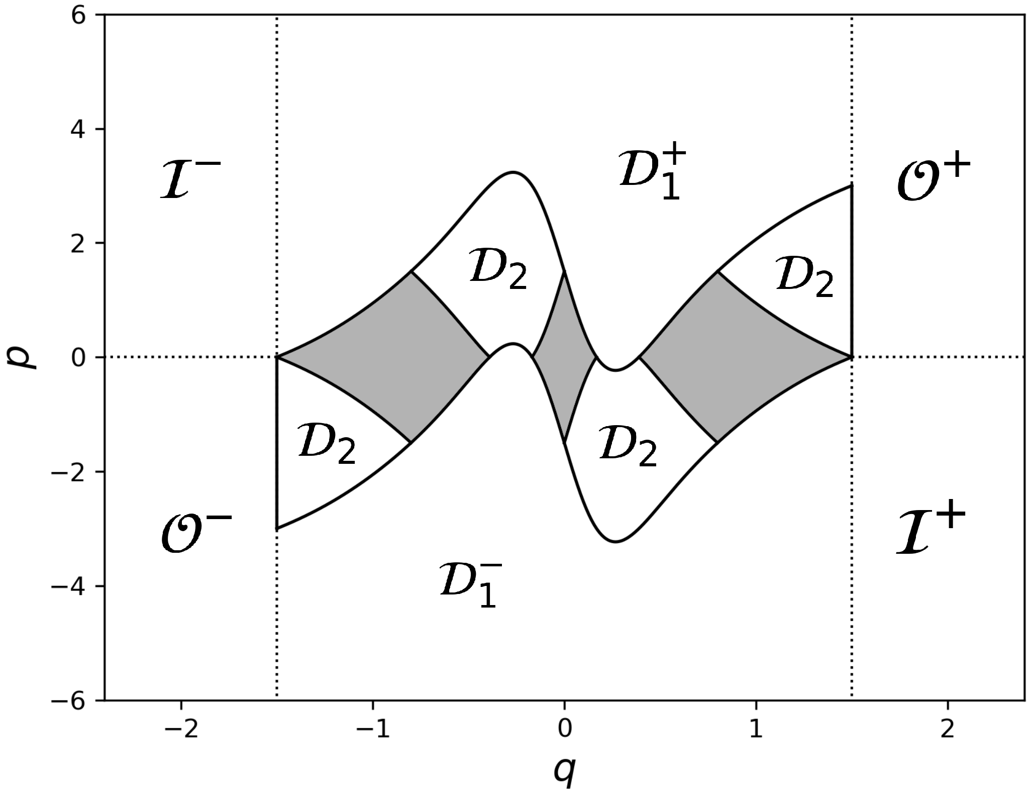
4. Non-Wandering Set and the Filtration Property

To show that the non-wandering set $\Omega \left(U\right)$ of the system is uniformly hyperbolic, here we prove that the non-wandering set $\Omega \left(U\right)$ is a subset of $R\cap U^{-1}\left(R\right)$ by showing that the complement of $R\cap U^{-1}\left(R\right)$ is wandering. To this end, we introduce the following regions,

$$\begin{array}{c}{\mathcal{O}}^{+}=\left\{(q,p)\right|q>q_f,p>0\},\hfill \end{array}$$

(31)

$$\begin{array}{c}{\mathcal{O}}^{-}=\left\{(q,p)\right|q<-q_f,p<0\},\hfill \end{array}$$

(32)

$$\begin{array}{c}{\mathcal{I}}^{+}=\left\{(q,p)\right|q>q_f,p<0\},\hfill \end{array}$$

(33)

$$\begin{array}{c}{\mathcal{I}}^{-}=\left\{(q,p)\right|q<-q_f,p>0\}.\hfill \end{array}$$

(34)

As shown in [12], these regions have the following properties.

Lemma 1.

If the condition,

$$\begin{array}{c}\hfill V^{\prime }\left(q\right)<0 \mathrm{for} q>q_f,\end{array}$$

(35)

is fulfilled, which automatically implies$V^{\prime }\left(q\right)>0$for$q<-q_f$because of the symmetry of the potential function, then we have

(a) 

$U\left({\mathcal{O}}^{+}\right)\subset {\mathcal{O}}^{+}$ and $U\left({\mathcal{O}}^{-}\right)\subset {\mathcal{O}}^{-}$.

(b) 

$q_n\in {\mathcal{O}}^{+}$ is strictly increasing, and $q_n\in {\mathcal{O}}^{-}$ is strictly decreasing under forward iteration of the map U.

(c) 

$U^{-1}\left({\mathcal{I}}^{+}\right)\subset {\mathcal{I}}^{+}$ and $U^{-1}\left({\mathcal{I}}^{-}\right)\subset {\mathcal{I}}^{-}$.

(d) 

$q_n\in {\mathcal{I}}^{+}$ is strictly increasing, and $q_n\in {\mathcal{I}}^{-}$ is strictly decreasing under backward iteration of the map U.

Proof. 

From the condition (35), $(q_n,p_n)\in {\mathcal{O}}^{+}$ satisfies

$$\begin{array}{c}\hfill q_{n+1}=q_n+p_n-\frac{1}{2}{V}^{\prime }\left(q_n\right)>q_n+p_n>q_n>q_f,\end{array}$$

(36)

and

$$\begin{array}{c}\hfill p_{n+1}=p_n-\frac{1}{2}{V}^{\prime }\left(q_n\right)-\frac{1}{2}{V}^{\prime }\left(q_{n+1}\right)>p_n>0,\end{array}$$

(37)

which implies $(q_{n+1},p_{n+1})\in {\mathcal{O}}^{+}$. Using the symmetry, the statements for ${\mathcal{O}}^{-},{\mathcal{I}}^{+}$ and ${\mathcal{I}}^{-}$ immediately follow. □

Remark. 

The condition holds true for fixed $q_b$ and $q_f$ (see (8)).

Next, we consider the behavior of the internal region $\left\{(q,p)\right|-q_f<q<q_f\}$ under the iteration. To this end, we focus on the forward and backward image of the complement of $R\cap U^{-1}\left(R\right)$, respectively. As shown in Figure 7, we introduce subsets (${\mathcal{C}}_1^{\pm },{\mathcal{C}}_2)$ as the forward image of the complement of $R\cap U^{-1}\left(R\right)$:

$$\begin{array}{c}{\mathcal{C}}_1^{+}=\left\{(q,p)\right|-q_f<q<q_f,p>-F\left(q\right)+2q_f\},\hfill \end{array}$$

(38)

$$\begin{array}{c}{\mathcal{C}}_1^{-}=\left\{(q,p)\right|-q_f<q<q_f,p<-F\left(q\right)\},\hfill \end{array}$$

(39)

$$\begin{array}{c}{\mathcal{C}}_2=U^{-1}\left(R\right)\backslash (R\cap U^{-1}\left(R\right)).\hfill \end{array}$$

(40)

As ${\mathcal{C}}_2\subset U^{-1}\left(R\right)$, $U\left({\mathcal{C}}_2\right)\subset R$ holds, thus $U\left({\mathcal{C}}_2\right)\subset (R\cap U^{-1}\left(R\right))\cup {\mathcal{C}}_1^{+}\cup {\mathcal{C}}_1^{-}$ follows. As for ${\mathcal{C}}_1^{\pm }$, we have the following lemma. The same proof is given in our forthcoming paper [19], but we explicitly state this to make the paper self-contained.

Lemma 2.

If the condition (35) is satisfied, then

$$\begin{array}{c}\hfill U\left({\mathcal{C}}_1^{+}\right)\subset {\mathcal{O}}^{+} and U\left({\mathcal{C}}_1^{-}\right)\subset {\mathcal{O}}^{-}.\end{array}$$

(41)

Proof. 

For $(q_n,p_n)\in {\mathcal{C}}_1^{+}$, we have

$$\begin{array}{c}\hfill q_{n+1}=q_n+p_n-\frac{1}{2}{V}^{\prime }\left(q_n\right)>q_f.\end{array}$$

(42)

Combining this with the condition (35), we can show that

$$\begin{array}{ccc}\hfill p_{n+1}& =& p_n-\frac{1}{2}{V}^{\prime }\left(q_n\right)-\frac{1}{2}{V}^{\prime }\left(q_{n+1}\right)\hfill \\ & >& -q_n+q_f-\frac{1}{2}{V}^{\prime }\left(q_{n+1}\right)\hfill \\ & >& -\frac{1}{2}{V}^{\prime }\left(q_{n+1}\right)>0.\hfill \end{array}$$

(43)

This implies $(q_{n+1},p_{n+1})\in {\mathcal{O}}^{+}$. One similarly shows that $U\left({\mathcal{C}}_1^{-}\right)\subset {\mathcal{O}}^{-}$. □

In a similar way, Figure 8 illustrates subsets (${\mathcal{D}}_1^{\pm },{\mathcal{D}}_2$), which are introduced as the backward image of the complement of $R\cap U^{-1}\left(R\right)$:

$$\begin{array}{c}{\mathcal{D}}_1^{+}=\left\{(q,p)\right|-q_f<q<q_f,p>F\left(q\right)\},\hfill \end{array}$$

(44)

$$\begin{array}{c}{\mathcal{D}}_1^{-}=\left\{(q,p)\right|-q_f<q<q_f,p<F\left(q\right)-2q_f\},\hfill \end{array}$$

(45)

$$\begin{array}{c}{\mathcal{D}}_2=R\backslash (R\backslash U^{-1}\left(R\right)).\hfill \end{array}$$

(46)

As ${\mathcal{D}}_2\subset R$, $U^{-1}\left({\mathcal{D}}_2\right)\subset U^{-1}\left(R\right)$ holds, $U^{-1}\left({\mathcal{D}}_2\right)\subset (R\cap U^{-1}\left(R\right))\cup {\mathcal{D}}_1^{+}\cup {\mathcal{D}}_1^{-}$ follows. As for ${\mathcal{D}}_1^{\pm }$, we have the lemma:

Lemma 3.

If the condition (35) is satisfied, then

$$\begin{array}{c}\hfill U^{-1}\left({\mathcal{D}}_1^{+}\right)\subset {\mathcal{I}}^{-} and U^{-1}\left({\mathcal{D}}_1^{-}\right)\subset {\mathcal{I}}^{+}.\end{array}$$

(47)

Proof. 

For $(q_n,p_n)\in {\mathcal{D}}_1^{+}$, we have

$$\begin{array}{c}\hfill q_{n-1}=q_n-p_n-\frac{1}{2}{V}^{\prime }\left(q_n\right)<-q_f.\end{array}$$

(48)

Combining this with the condition (35), this leads to

$$\begin{array}{ccc}\hfill p_{n-1}& =& p_n+\frac{1}{2}{V}^{\prime }\left(q_n\right)+\frac{1}{2}{V}^{\prime }\left(q_{n-1}\right)\hfill \\ & >& q_n+q_f+\frac{1}{2}{V}^{\prime }\left(q_{n-1}\right)>0.\hfill \end{array}$$

(49)

This implies $(q_{n-1},p_{n-1})\in {\mathcal{I}}^{-}$. One similarly show that $U^{-1}\left({\mathcal{D}}_1^{-}\right)\subset {\mathcal{I}}^{+}$. □

Considering the behavior of the complement of $R\cap U^{-1}\left(R\right)$ under forward/backward iterations of U, we arrive at the following.

Proposition 2.

If the condition (35) is satisfied, $\Omega \left(U\right)\subset R\cap U^{-1}\left(R\right)$ holds.

Proof. 

From the lemmas (1), (2), and (3), we can say that the complement of the set $R\cap U^{-1}\left(R\right)$ is wandering. □

As numerically confirmed in Figure 9, heteroclinic points associated with stable and unstable manifolds for fixed points are actually contained in the region $R\cap U^{-1}\left(R\right)$.

5. Sector Condition

We first give the definition for the uniform hyperbolicity and also provide a sufficient condition for the system to be uniformly hyperbolic.

Definition 1.

The diffeomorphism U defined on a manifold M said to be uniformly hyperbolic if for any $x\in M$ the associated tangent space is decomposed into stable and unstable spaces as $T_{x}M=E^s\left(x\right)⨁E^u\left(x\right)$, and for any $n\in \mathbb{N}$ there exist constants $C>0$ and $\lambda \in (0,1)$ such that

$$\begin{array}{c}\hfill \parallel D{U}^n\left(\nu \right)\parallel \le C{\lambda }^n\parallel \nu \parallel for \nu \in E^s\left(x\right) and \parallel D{U}^{-n}\left(\nu \right)\parallel \le C{\lambda }^n\parallel \nu \parallel for \nu \in E^u\left(x\right)\end{array}$$

(50)

holds.

As is well known, so-called the sector condition provides a sufficient condition for the uniform hyperbolicity [20]. The sector condition is formulated as having the sector bundles

$$\begin{array}{c}{S}_{\lambda }^{+}=\left\{(\xi ,\eta )\right|\left|\xi \right|\ge \lambda \left|\eta \right|\},\hfill \end{array}$$

(51)

$$\begin{array}{c}{S}_{\lambda }^{-}=\left\{(\xi ,\eta )\right|\lambda \left|\eta \right|\le \left|\xi \right|\},\hfill \end{array}$$

(52)

with a certain $\lambda >1$.

Here, we first show the Jacobians $JU$ for the map U and $J{U}^{-1}$ for the inverse map $U^{-1}$:

$$\begin{array}{ccc}\hfill J{U}_{(q_n,p_n)}& =& \left(\begin{array}{cc}\frac{{\displaystyle \partial q_{n+1}}}{{\displaystyle \partial q_n}}& \frac{{\displaystyle \partial q_{n+1}}}{{\displaystyle \partial p_n}}\\ \frac{{\displaystyle \partial p_{n+1}}}{{\displaystyle \partial q_n}}& \frac{{\displaystyle \partial p_{n+1}}}{{\displaystyle \partial p_n}}\end{array}\right)\hfill \\ & =& \left(\begin{array}{cc}1-\frac{1}{2}{V}^{″}\left(q_n\right)& 1\\ -\frac{1}{2}{V}^{″}\left(q_n\right)-\frac{1}{2}{V}^{″}\left(q_{n+1}\right)(1-\frac{1}{2}{V}^{″}\left(q_n\right))& -\frac{1}{2}{V}^{″}\left(q_{n+1}\right)\end{array}\right)\hfill \\ & =& \left(\begin{array}{cc}\alpha \left(q_n\right)& 1\\ \alpha \left(q_n\right)\alpha \left(q_{n+1}\right)-1& \alpha \left(q_{n+1}\right)\end{array}\right),\hfill \end{array}$$

(53)

$$\begin{array}{ccc}\hfill J{U}_{(q_{n+1},p_{n+1})}^{-1}& =& \left(\begin{array}{cc}\alpha \left(q_{n+1}\right)& -1\\ 1-\alpha \left(q_n\right)\alpha \left(q_{n+1}\right)& \alpha \left(q_n\right)\end{array}\right),\hfill \end{array}$$

(54)

where

$$\begin{array}{ccc}\hfill \alpha \left(q\right)& :=& 1-\frac{1}{2}{V}^{″}\left(q\right)\hfill \\ \hfill & =& 1+\kappa \left\{\frac{4(12q^2-1)}{{(1+4q^2)}^3}-\epsilon \left(\frac{3{(q-q_b)}^2-1}{{(1+{(q-q_b)}^2)}^3}+\frac{3{(q+q_b)}^2-1}{{(1+{(q+q_b)}^2)}^3}\right)\right\}.\hfill \end{array}$$

Below, we drop the subscript $(q_n,p_n)$ if there is no confusion.

For the Hénon map, the sector condition can simply be written in terms of the original tangent space variables $(\xi ,\eta )$ [10], but for the present map verifying the sector condition for the original tangent space is not straightforward. Therefore, we transform the original tangent space $(\xi ,\eta )$ into $({\xi }^{\prime },{\eta }^{\prime })$ via the transformation

$$\begin{array}{c}\hfill T=\left(\begin{array}{cc}1& 1\\ 1-\alpha \left(q_n\right)\alpha \left(q_{n+1}\right)+\alpha \left(q_{n+1}\right)& \alpha \left(q_n\right)-1\end{array}\right),\end{array}$$

(55)

which yields the Jacobian $JU$ as

$$\begin{array}{ccc}\hfill J{U}^{\prime }& =& T\left(JU\right)T^{-1}\hfill \\ & =& \left(\begin{array}{cc}\alpha \left(q_n\right)+\alpha \left(q_{n+1}\right)& -1\\ 1& 0\end{array}\right),\hfill \end{array}$$

(56)

and the Jabocian $J{U}^{-1}$ for the inverse map as

$$\begin{array}{ccc}\hfill J{U}^{\prime -1}& =& T\left(J{U}^{-1}\right)T^{-1}\hfill \\ & =& \left(\begin{array}{cc}0& 1\\ -1& \alpha \left(q_n\right)+\alpha \left(q_{n+1}\right)\end{array}\right).\hfill \end{array}$$

(57)

To show the sector condition presented below, we prepare the following lemma.

Lemma 4.

For some $\lambda >1$ if

$$\begin{array}{c}\hfill |\alpha \left(q_n\right)+\alpha \left(q_{n+1}\right)|\ge 2\lambda \end{array}$$

(58)

is satisfied, then

(a) for any vector $({\xi }_n^{\prime },{\eta }_n^{\prime })\in S_{\lambda }^{\prime +}$, the vector $({\xi }_{n+1}^{\prime },{\eta }_{n+1}^{\prime })=J{U}^{\prime }({\xi }_n^{\prime },{\eta }_n^{\prime })$ satisfies $|{\xi }_{n+1}^{\prime }|>\lambda |{\xi }_n^{\prime }|$.

(b) for any vector $({\xi }_{n+1}^{\prime },{\eta }_{n+1}^{\prime })\in S_{\lambda }^{\prime -}$, the vector $({\xi }_n^{\prime },{\eta }_n^{\prime })=J{U}^{\prime -1}({\xi }_{n+1}^{\prime },{\eta }_{n+1}^{\prime })$ satisfies $|{\eta }_n^{\prime }|>\lambda |{\eta }_{n+1}^{\prime }|$.

Here the sector bundles are defined as

$$\begin{array}{ccc}\hfill S_{\lambda }^{\prime +}& =& \left\{({\xi }^{\prime },{\eta }^{\prime })\right|\left|{\xi }^{\prime }\right|\ge \lambda \left|{\eta }^{\prime }\right|\},\hfill \\ \hfill S_{\lambda }^{\prime -}& =& \left\{({\xi }^{\prime },{\eta }^{\prime })\right|\lambda \left|{\xi }^{\prime }\right|\le \left|{\eta }^{\prime }\right|\}.\hfill \end{array}$$

(59)

Proof. 

For (a), as

$$\begin{array}{ccc}\hfill \left(\begin{array}{c}{\xi }_{n+1}^{\prime }\\ {\eta }_{n+1}^{\prime }\end{array}\right)& =& J{U}^{\prime }\left(\begin{array}{c}{\xi }_n^{\prime }\\ {\eta }_n^{\prime }\end{array}\right)\hfill \\ & =& \left(\begin{array}{c}(\alpha \left(q_n\right)+\alpha \left(q_{n+1}\right)){\xi }_n^{\prime }-{\eta }_n^{\prime }\\ {\xi }_n^{\prime }\end{array}\right),\hfill \end{array}$$

(60)

we have

$$\begin{array}{ccc}\hfill |{\xi }_{n+1}^{\prime }|& =& |(\alpha \left(q_n\right)+\alpha \left(q_{n+1}\right)){\xi }_n^{\prime }-{\eta }_n^{\prime }|\hfill \\ & \ge & |\alpha \left(q_n\right)+\alpha \left(q_{n+1}\right)\left|\right|{\xi }_n^{\prime }|-|{\eta }_n^{\prime }|\hfill \\ & \ge & |\alpha \left(q_n\right)+\alpha \left(q_{n+1}\right)\left|\right|{\xi }_n^{\prime }|-\frac{1}{\lambda }\left|{\xi }_n^{\prime }\right|\hfill \\ & >& |\alpha \left(q_n\right)+\alpha \left(q_{n+1}\right)\left|\right|{\xi }_n^{\prime }|-\lambda |{\xi }_n^{\prime }|\hfill \\ & \ge & \lambda |{\xi }_n^{\prime }|.\hfill \end{array}$$

We have used (58) to show the last inequality. We can show (b) in a similar way. □

Using this lemma, we can easily see that the condition (58) provides the sector condition:

Proposition 3.

Suppose that, for $\lambda >1$, $\alpha \left(q_n\right),\alpha \left(q_{n+1}\right)$ satisfy

$$\begin{array}{c}\hfill |\alpha \left(q_n\right)+\alpha \left(q_{n+1}\right)|\ge 2\lambda ,\end{array}$$

(61)

then,

(a) for any vector $({\xi }_n^{\prime },{\eta }_n^{\prime })\in S_{\lambda }^{\prime +}$, the vector $({\xi }_{n+1}^{\prime },{\eta }_{n+1}^{\prime })=J{U}^{\prime }({\xi }_n^{\prime },{\eta }_n^{\prime })\in S_{\lambda }^{\prime +}$ and $|({\xi }_{n+1}^{\prime },{\eta }_{n+1}^{\prime })|\ge \lambda |({\xi }_n^{\prime },{\eta }_n^{\prime })|$ hold.

(b) for any vector $({\xi }_{n+1}^{\prime },{\eta }_{n+1}^{\prime })\in S_{\lambda }^{\prime -}$, the vector $({\xi }_n^{\prime },{\eta }_n^{\prime })=J{U}^{\prime -1}({\xi }_{n+1}^{\prime },{\eta }_{n+1}^{\prime })\in S_{\lambda }^{\prime -}$ and $|({\xi }_n^{\prime },{\eta }_n^{\prime })|\ge \lambda |({\xi }_{n+1}^{\prime },{\eta }_{n+1}^{\prime })|$ hold.

Proof. 

For (a), using Lemma 4 and (60), we have

$$\begin{array}{ccc}\hfill |{\xi }_{n+1}^{\prime }|& >& \lambda |{\xi }_n^{\prime }|\hfill \\ & =& \lambda |{\eta }_{n+1}^{\prime }|.\hfill \end{array}$$

(62)

This implies $({\xi }_{n+1}^{\prime },{\eta }_{n+1}^{\prime })\in S_{\lambda }^{\prime +}$. In addition, since $|{\xi }_n^{\prime }|\ge \lambda |{\eta }_n^{\prime }|$, we have

$$\begin{array}{ccc}\hfill |{\eta }_{n+1}^{\prime }|& =& |{\xi }_n^{\prime }|\hfill \\ & \ge & \lambda |{\eta }_n^{\prime }|.\hfill \end{array}$$

(63)

This leads, together with Lemma 4, to $|({\xi }_{n+1}^{\prime },{\eta }_{n+1}^{\prime })|\ge \lambda |({\xi }_n^{\prime },{\eta }_n^{\prime })|$. We can show (b) in a similar manner. □

6. Sufficient Condition for the Sector Condition

6.1. Numerical Observation for the Sector Condition

Now we seek in which situations the condition (58) is satisfied. Before going to develop analytical arguments, we present some numerical observations demonstrating how the region where the condition (58) is satisfied behaves. As observed in Figure 10, there exist regions not satisfying the condition (58) in the $R\cap U^{-1}\left(R\right)$. Therefore, we are not able to expect the uniform hyperbolicity in the whole $R\cap U^{-1}\left(R\right)$ region. On the other hand, Figure 11 implies that the uniform hyperbolicity holds in $R\cap U^{-1}\left(R\right)\cap U^{-2}\left(R\right)$. To push this idea, herein we introduce more proper domains that make it possible to write down explicit conditions for the uniform hyperbolicity because the boundary curves for $R\cap U^{-1}\left(R\right)\cap U^{-2}\left(R\right)$ are not analytically tractable.

6.2. Preliminary for the Division of the Phase Space

Instead of considering the uniform hyperbolicity for the domain $R\cap U^{-1}\left(R\right)\cap U^{-2}\left(R\right)$, we here show that the region, which contains the domain $R\cap U^{-1}\left(R\right)\cap U^{-2}\left(R\right)$ and can more easily be accessed, satisfies the condition (58). To specify such a region, we introduce the following function,

$$\begin{array}{c}\hfill L\left(q\right):=\kappa q\left(\frac{100\sqrt{5}}{27}q-4\right)+2q_f+\kappa \epsilon c_1,\end{array}$$

(64)

which provides an upper bound of $F\left(q\right)$ (see Figure 12). Using the inequality valid for $q>0$,

$$\begin{array}{c}\hfill -\frac{4}{{(1+4q^2)}^2}<\frac{100\sqrt{5}}{27}q-4,\end{array}$$

(65)

we can show that the following holds,

$$\begin{array}{c}\hfill 2q_f-\frac{3\sqrt{3}}{8}\kappa +\kappa \epsilon c_1<L\left(q\right).\end{array}$$

(66)

Together with the upper bound for $F\left(q\right)$, it is easy to see that the relation

$$\begin{array}{c}\hfill F\left(q\right)<L\left(q\right)\end{array}$$

(67)

holds. Here, ${\omega }_1$ and ${\omega }_2$ are the solutions of the following quadratic equation $L\left(q\right)=0$ (see Figure 13),

$$\begin{array}{c}\hfill {\omega }_1=c_2-\sqrt{{c_2}^2-\frac{1}{2}{c}_2{c}_1\epsilon -c_2{q}_f\frac{1}{\kappa }},\end{array}$$

(68)

$$\begin{array}{c}\hfill {\omega }_2=c_2+\sqrt{{c_2}^2-\frac{1}{2}{c}_2{c}_1\epsilon -c_2{q}_f\frac{1}{\kappa }},\end{array}$$

(69)

where

$$\begin{array}{c}\hfill c_2:=\frac{27}{50\sqrt{5}}.\end{array}$$

(70)

Here, we introduce the notation for the discriminant as

$$\begin{array}{c}\hfill \Delta (\kappa ,q_b,q_f):={c_2}^2-\frac{1}{2}{c}_2{c}_1\epsilon -c_2{q}_f\frac{1}{\kappa }.\end{array}$$

(71)

So that ${\omega }_1$ and ${\omega }_2$ are both real, the condition

$$\begin{array}{c}\hfill \kappa >\frac{2q_f}{{\displaystyle 2c_2-c_1\epsilon }}\end{array}$$

(72)

must be satisfied.

6.3. Division of the Phase Space

To find sufficient conditions leading to the condition (58), we first divide the phase space into three subregions (see Figure 14):

$$\begin{array}{ccc}\hfill \overline{\mathcal{X}}& =& \left\{(q,p)\right|-q_f<q<-{\omega }_2\},\hfill \end{array}$$

(73)

$$\begin{array}{ccc}\hfill \overline{\mathcal{Y}}& =& \left\{(q,p)\right|-{\omega }_1<q<{\omega }_1\},\hfill \end{array}$$

(74)

$$\begin{array}{ccc}\hfill \overline{\mathcal{Z}}& =& \left\{(q,p)\right|{\omega }_2<q<q_f\}.\hfill \end{array}$$

(75)

In the following, we will examine a region which contains the non-wandering set of the map U and find the parameter regions in which the condition (58) holds. First note that $R\cap U^{-1}\left(R\right)\subset \overline{\mathcal{X}}\cup \overline{\mathcal{Y}}\cup \overline{\mathcal{Z}}$ trivially holds because of the definition for ${\omega }_1$ and ${\omega }_2$. Combined with the Proposition 2, this immediately leads to $U(\Omega \left(U\right))=\Omega \left(U\right)\subset \overline{\mathcal{X}}\cup \overline{\mathcal{Y}}\cup \overline{\mathcal{Z}}$. As the non-wandering set $\Omega \left(U\right)$ is an invariant set, $U(\Omega \left(U\right))=\Omega \left(U\right)\subset \overline{\mathcal{X}}\cup \overline{\mathcal{Y}}\cup \overline{\mathcal{Z}}$ holds. Therefore, we have $\Omega \left(U\right)\subset (\overline{\mathcal{X}}\cup \overline{\mathcal{Y}}\cup \overline{\mathcal{Z}})\cap U^{-1}(\overline{\mathcal{X}}\cup \overline{\mathcal{Y}}\cup \overline{\mathcal{Z}})$. Consequently, we can say that if the set $(\overline{\mathcal{X}}\cup \overline{\mathcal{Y}}\cup \overline{\mathcal{Z}})\cap U^{-1}(\overline{\mathcal{X}}\cup \overline{\mathcal{Y}}\cup \overline{\mathcal{Z}})$ satisfies the sector condition (58), then the non-wandering set $\Omega \left(U\right)$ also satisfies it, implying that $\Omega \left(U\right)$ is uniformly hyperbolic. In subsequent arguments, as illustrated in Figure 15, we will explore the parameter regions in which the points

$$\begin{array}{c}\hfill (q_n,p_n)\in U^{-1}(\overline{\mathcal{X}}\cup \overline{\mathcal{Y}}\cup \overline{\mathcal{Z}})\cap (\overline{\mathcal{X}}\cup \overline{\mathcal{Y}}\cup \overline{\mathcal{Z}})\end{array}$$

(76)

satisfy the sector condition (58).

6.4. Sufficient Conditions for the Sector Condition

We now analyze the following three situations and ask the condition leading to the sector condition (58).

(Case 1)$q_n,q_{n+1}\in \overline{\mathcal{Y}}$.

(Case 2)$q_n,q_{n+1}\in \overline{\mathcal{X}}\cup \overline{\mathcal{Z}}$.

(Case 3)$q_n\in \overline{\mathcal{X}}\cup \overline{\mathcal{Z}}$ and $q_{n+1}\in \overline{\mathcal{Y}}$, or $q_n\in \overline{\mathcal{Y}}$ and $q_{n+1}\in \overline{\mathcal{X}}\cup \overline{\mathcal{Z}}$.

Note that these are all possible patterns that can occur. Due to the symmetry of the function $\alpha \left(q\right)$ with respect to the p-axis, it is sufficient to consider the condition only for the right half of phase space, that is, the region $q>0$ in $\overline{\mathcal{Y}}$ and $\overline{\mathcal{Z}}$.

6.4.1. Case 1

We here consider the case where $(q_n,p_n)$ and $(q_{n+1},p_{n+1})\in \overline{\mathcal{Y}}$. Since $-1\le (3q^2-1)/{(1+q^2)}^3\le 1/4$ holds, we have

$$\begin{array}{c}\hfill \alpha \left(q\right)\le {\beta }_1\left(q\right),\end{array}$$

(77)

where

$$\begin{array}{c}\hfill {\beta }_1\left(q\right):=1+\kappa \frac{4(12q^2-1)}{{(1+4q^2)}^3}+2\kappa \epsilon .\end{array}$$

(78)

Note that

$$\begin{array}{c}\hfill \frac{d{\beta }_1\left(q\right)}{dq}=\kappa \frac{192q(1-4q^2)}{{(1+4q^2)}^4},\end{array}$$

(79)

and the function ${\beta }_1\left(q\right)$ has extrema at $q=0,\pm 1/2$. But since $0<{\omega }_1<1/2$, ${\beta }_1\left(q\right)$ monotonically increases in the region $\overline{\mathcal{Y}}$, ${\beta }_1\left(q\right)$ becomes maximal at $q={\omega }_1$. Therefore, if ${\beta }_1\left({\omega }_1\right)<-1$, then $\left|\alpha \right(q\left)\right|>1$ follows. This immediately leads to the condition (58). The condition ${\beta }_1\left({\omega }_1\right)<-1$ is explicitly written as

$$\begin{array}{c}\hfill 2+\kappa \frac{4(12{{\omega }_1}^2-1)}{{(1+4{{\omega }_1}^2)}^3}+2\kappa \epsilon <0.\end{array}$$

(80)

6.4.2. Case 2

Next, we consider the case when both $(q_n,p_n)$ and $(q_{n+1},p_{n+1})\in \overline{\mathcal{Z}}$. As $1\le q_b$, the function $(3{(q+q_b)}^2-1)/{(1+{(q+q_b)}^2)}^3$ monotonically decreases for $q>0$. Combining the fact that $-1\le (3{(q-q_b)}^2-1)/{(1+{(q-q_b)}^2)}^3\le 1/4$ holds, we can show that

$$\begin{array}{c}\hfill \alpha \left(q\right)>{\beta }_2\left(q\right),\end{array}$$

(81)

where

$$\begin{array}{c}\hfill {\beta }_2\left(q\right):=1+\kappa \frac{4(12q^2-1)}{{(1+4q^2)}^3}-\left(\frac{1}{4}+\frac{3q_b^2-1}{{(1+q_b^2)}^3}\right)\kappa \epsilon .\end{array}$$

(82)

Note that

$$\begin{array}{c}\hfill \frac{d{\beta }_2\left(q\right)}{dq}=\kappa \frac{192q(1-4q^2)}{{(1+4q^2)}^4},\end{array}$$

(83)

and $c_2<{\omega }_2<2c_2$ with $2c_2\approx 0.4829\cdots$, it is easy to show that ${\beta }_2\left(q\right)$ is an increasing function in the interval ${\omega }_2<q<1/2$, while it decreases in the rest of the interval $1/2<q<q_f$. Therefore if ${\beta }_2\left({\omega }_2\right)>1$ and ${\beta }_2\left(q_f\right)>1$ are satisfied, $\alpha \left(q\right)>{\beta }_2\left(q\right)>1$ holds, which leads to the condition (58). A concrete expression for the condition ${\beta }_2\left({\omega }_2\right)>1$ is written as

$$\begin{array}{c}\hfill \kappa \frac{4(12{{\omega }_2}^2-1)}{{(1+4{{\omega }_2}^2)}^3}-\left(\frac{1}{4}+\frac{3q_b^2-1}{{(1+q_b^2)}^3}\right)\kappa \epsilon >0,\end{array}$$

(84)

and the condition ${\beta }_2\left(q_f\right)>1$ is expressed as

$$\begin{array}{c}\hfill \kappa \frac{4(12{q_f}^2-1)}{{(1+4{q_f}^2)}^3}-\left(\frac{1}{4}+\frac{3q_b^2-1}{{(1+q_b^2)}^3}\right)\kappa \epsilon >0.\end{array}$$

(85)

For an explicit value $(q_b,q_f)=(1.0,1.5)$, we have

$$\begin{array}{c}\hfill \frac{4(12{q_f}^2-1)}{{(1+4{q_f}^2)}^3}-\left(\frac{1}{4}+\frac{3q_b^2-1}{{(1+q_b^2)}^3}\right)\epsilon \approx 0.0223\cdots >0,\end{array}$$

which implies that the condition (85) holds for $\kappa >0$.

6.4.3. Case 3

Suppose here that $(q_n,p_n)\in \overline{\mathcal{Z}}$ and $(q_{n+1},p_{n+1})\in \overline{\mathcal{Y}}$. Because of the inequality (77), we have

$$\begin{array}{c}\hfill \alpha \left(q_0\right)<\underset{0<q<q_f}{max}{\beta }_1\left(q\right)={\beta }_1(1/2)=1+\kappa +2\kappa \epsilon .\end{array}$$

(86)

On the other hand, if ${\beta }_1\left(q_{n+1}\right)<-2-{\beta }_1(1/2)$ holds, then $\alpha \left(q_{n+1}\right)<-2-{\beta }_1(1/2)$ follows due to the inequality (77), which then leads to the condition $\alpha \left(q_n\right)+\alpha \left(q_{n+1}\right)<-2$. Note that $0<{\omega }_1<1/2$, so ${\beta }_1\left(q_{n+1}\right)$ monotonically increases for $(q_{n+1},p_{n+1})\in \overline{\mathcal{Y}}$. Therefore, if ${\beta }_1\left({\omega }_1\right)<-2-{\beta }_1(1/2)$, then the inequality ${\beta }_1\left(q_{n+1}\right)<-2-{\beta }_1(1/2)$ holds for $(q_{n+1},p_{n+1})\in \overline{\mathcal{Y}}$. Therefore, the condition ${\beta }_1\left({\omega }_1\right)<-2-{\beta }_1(1/2)$ is a sufficient condition for (58). We can write this condition explicitly as

$$\begin{array}{c}\hfill 4+\kappa \frac{4(12{{\omega }_1}^2-1)}{{(1+4{{\omega }_1}^2)}^3}+\kappa +4\kappa \epsilon <0.\end{array}$$

(87)

Obviously, because

$$\begin{array}{c}\hfill {\beta }_1(1/2)=1+\kappa +2\kappa \epsilon >0,\end{array}$$

(88)

the condition (80) is automatically satisfied if the condition (87) is satisfied, so it turns out that the condition (80) becomes redundant. As a result, we can say that if the conditions (84), (85), and (87) hold, the sector condition (58) is satisfied.

6.5. The Condition for Case 2

The condition (84) is rewritten as

$$\begin{array}{c}\hfill \kappa \frac{4(12{{\omega }_2}^2-1)}{{(1+4{{\omega }_2}^2)}^3}-\left(\frac{1}{4}+\frac{3q_b^2-1}{{(1+q_b^2)}^3}\right)\kappa \epsilon >0.\end{array}$$

(89)

Here, we use our initial assumption $\kappa >0$. As $0<c_2<{\omega }_2<2c_2$, we have ${(1+4{{\omega }_2}^2)}^{-3}>{\left(1+4{\left(2c_2\right)}^2\right)}^{-3}$, so in order to show the inequality (89), it is sufficient to show

$$\begin{array}{c}\hfill \kappa \frac{4(12{{\omega }_2}^2-1)}{{\displaystyle {\left(1+{4\left(2c_2\right)}^2\right)}^3}}-\left(\frac{1}{4}+\frac{3q_b^2-1}{{(1+q_b^2)}^3}\right)\kappa \epsilon >0.\end{array}$$

(90)

This can be explicitly written as

$$\begin{array}{c}\hfill c_2^2+2c_2\sqrt{\Delta (\kappa ,q_b,q_f)}+\Delta (\kappa ,q_b,q_f)>\frac{1}{12}+\epsilon \frac{{\left(1+16c_2^2\right)}^3}{48}\left(\frac{1}{4}+\frac{3q_b^2-1}{{(1+q_b^2)}^3}\right).\end{array}$$

(91)

The condition ensuring that ${\omega }_1$ and ${\omega }_2$ are both real, we have $c_2>\sqrt{\Delta }$, which leads to

$$\begin{array}{c}\hfill c_2\sqrt{\Delta }>\Delta .\end{array}$$

(92)

Therefore the left-hand side of the inequality (91) is larger than $c_2^2+3\Delta$. By replacing the left-hand side of (91) by $c_2^2+3\Delta$, an explicit condition for $\kappa$ is then obtained as

$$\begin{array}{c}\hfill \kappa >\frac{{\displaystyle 12c_2{q}_f}}{{\displaystyle 16c_2^2-\frac{1}{3}-\epsilon \left(6c_1{c}_2+\frac{{\left(1+16c_2^2\right)}^3}{12}\left(\frac{1}{4}+\frac{3q_b^2-1}{{(1+q_b^2)}^3}\right)\right)}}.\end{array}$$

(93)

6.6. The Condition for Case 3

As $0<{\omega }_1<c_2$, we have $(12{{\omega }_1}^2-1)<0$ and ${(1+4{{\omega }_1}^2)}^{-3}>{\left(1+4{c_2}^2\right)}^{-3}$. Therefore the condition (87) is fulfilled if

$$\begin{array}{c}\hfill \kappa \left(\frac{4(12{{\omega }_1}^2-1)}{{\left(1+4c_2^2\right)}^3}+1+4ϵ\right)+4<0\end{array}$$

(94)

is satisfied. Recall that

$$\begin{array}{c}\hfill {{\omega }_1}^2=c_2^2-2c_2\sqrt{\Delta (\kappa ,q_b,q_f)}+\Delta (\kappa ,q_b,q_f).\end{array}$$

Using the inequality (92), we obtain

$$\begin{array}{ccc}\hfill {{\omega }_1}^2& <& c_2^2-\Delta \hfill \\ & =& \frac{1}{2}{c}_2{c}_1\epsilon +2c_2{q}_f\frac{1}{\kappa }.\hfill \end{array}$$

(95)

Introducing

$$\begin{array}{c}\hfill \delta \left(\kappa \right):=\frac{{\displaystyle 4\left(12\left(\frac{1}{2}{c}_2{c}_1\epsilon +2c_2{q}_f\frac{1}{\kappa }\right)-1\right)}}{{\left(1+4c_2^2\right)}^3}+1+4ϵ,\end{array}$$

and using (95), we have

$$\begin{array}{c}\hfill \frac{4(12{{\omega }_1}^2-1)}{{\left(1+4c_2^2\right)}^3}+1+4\epsilon <\delta \left(\kappa \right).\end{array}$$

(96)

Therefore if $\kappa \delta \left(\kappa \right)+4<0$, the inequality (94) holds true. This can be rewritten for the condition for $\kappa$ as

$$\begin{array}{c}\hfill \kappa >\frac{{\left(1+4c_2^2\right)}^3+12c_2{q}_f}{{\displaystyle 1-\frac{1}{4}{\left(1+4c_2^2\right)}^3-\epsilon \left(6c_1{c}_2+{\left(1+4c_2^2\right)}^3\right)}}\end{array}$$

(97)

Summarizing, if the following inequalities are satisfied, the sector condition (58) holds.

$$\begin{array}{c}\hfill \kappa >\frac{{\left(1+4c_2^2\right)}^3+12c_2{q}_f}{{\displaystyle 1-\frac{1}{4}{\left(1+4c_2^2\right)}^3-\epsilon \left(6c_1{c}_2+{\left(1+4c_2^2\right)}^3\right)}}\approx 69.9923\cdots .\end{array}$$

(98)

7. Conclusions

In this paper, we have provided a sufficient condition for the topological horseshoe and uniform hyperbolicity for the 2-dimensional area-preserving map in which the potential function is expressed by Lorentzian functions.

The proposed model could be an ideal model to explore several open problems in physics. As we mentioned in introduction, our scattering system well fits to the test of the fractal Weyl law conjecture. The resonances have been computed using a well-established numerical scheme such as the complex scaling method [12]. Note that resonances are sensitive to analytic property of the potential function, so one has to prepare well-controlled systems to see Planck constant’s dependence of resonances [12].

The scattering map proposed here can be used to investigate another fundamental problem in physics. Quantum tunneling in non-integrable systems has extensively been studied for the past decades [21], but the issue is still controversial because the role of chaos in phase space is not clear enough especially when one focuses on the nature of tunneling in the energy domain. Our scattering map exhibits mixed phase space when $\kappa$ is small, so it provides a good testing ground for the study of dynamical tunneling in terms of the complex semiclassical method [22,23]. In particular, the imaginary part of resonances of the scattering system is expected to represent the tunneling probability if one prepares the classical phase space in a proper way. In that situation, we have a chance to apply the complex semiclassical calculation to obtain the imaginary part of resonances while phase space for closed systems is too complicated to perform such an analysis.

Note that the condition for the parameter $\kappa$ is far from optimal. As illustrated in Figure 16, numerical calculations for stable and unstable manifolds show that the topological horseshoe and uniform hyperbolicity are achieved when $\kappa \gtrsim 1.8$ while the estimation made above predicts $\kappa \gtrsim 70.0$.

Throughout this paper, we have fixed the parameter values for $q_b$ and $q_f$ and derived a condition only for $\kappa$, in which the topological horseshoe and uniform hyperbolicity hold. However, it would be interesting to examine the whole parameter regions including $q_b$ and $q_f$.

Another extension could be made by by putting a parameter $\tau$ as

$$\begin{array}{c}\hfill f_1(q;\tau )\equiv \frac{1}{1+\tau q^2}.\end{array}$$

(99)

In the case studied in this paper, we have taken $\tau =4$. However, for $\tau =1$, a numerical computation strongly suggests that the system is no more uniformly hyperbolic if the same parameter set $(q_b,q_f)$ is chosen, implying that the nature of dynamics in not necessarily monotonic and simple in the whole parameter space.