Evaluating Superconductors through Current Induced Depairing

Abstract

The phenomenon of superconductivity occurs in the phase space of three principal parameters: temperature T, magnetic field B, and current density j. The critical temperature $T_c$ is one of the first parameters that is measured and in a certain way defines the superconductor. From the practical applications point of view, of equal importance is the upper critical magnetic field $B_{c2}$ and conventional critical current density $j_c$ (above which the system begins to show resistance without entering the normal state). However, a seldom-measured parameter, the depairing current density $j_d$, holds the same fundamental importance as $T_c$ and $B_{c2}$, in that it defines a boundary between the superconducting and normal states. A study of $j_d$ sheds unique light on other important characteristics of the superconducting state such as the superfluid density and the nature of the normal state below $T_c$, information that can play a key role in better understanding newly-discovered superconducting materials. From a measurement perspective, the extremely high values of $j_d$ make it difficult to measure, which is the reason why it is seldom measured. Here, we will review the fundamentals of current-induced depairing and the fast-pulsed current technique that facilitates its measurement and discuss the results of its application to the topological-insulator/chalcogenide interfacial superconducting system.

The phenomenon of superconductivity has a long and rich history: from the initial discovery in 1911 of superconductivity in mercury at liquid-helium temperature [1] to the recent discovery of room-temperature superconductivity in lanthanum superhydride [2,3]. Numerous parameters, probed by a variety of techniques, are used to characterize the superconducting state. However, the mixed-state upper critical field $B_{c2}$, reflective of the coherence length $\xi$, and the penetration depth ${\lambda }_L$, reflective of the superfluid density ${\rho }_s$=$1/{\lambda }^2$, are two crucial measurements that are amongst the first to be performed. There are multiple techniques for determining such parameters, each of which has its own advantages and limitations. Our group has developed some uncommon, and in some cases unique, experimental techniques that investigate superconductors at ultra-short time scales, and under unprecedented and extreme conditions of current density j, electric fields E, and power density $p=\rho j^2$ (where $\rho$ is the resistivity). These techniques have led to the discovery or confirmation of several novel phenomena and regimes in superconductors and in addition provide an alternative method to glean information on fundamental superconducting parameters, which in some cases may be hard to obtain by other methods. These methods and approaches are highly relevant in the search for new superconducting materials and in developing an understanding of their fundamental properties. This article discusses the physical meaning of $j_d$ and its interrelationships with other basic parameters of the superconducting state, as well as the technical challenges in measuring this important critical parameter. We discuss our results from this approach in the study of the topological-insulator/chalcogenide interfacial superconducting system.

1. Introduction

Attractive interactions between charge carriers cause them to condense by pairs into a coherent macroscopic quantum state below some transition temperature $T_c$. The formation of this state is governed principally by a competition between four energies: condensation, magnetic-field expulsion, thermal, and kinetic. The order parameter $\Delta$, which describes the extent of condensation and the strength of the superconducting state, is reduced as the temperature T, magnetic field B, and electric current density j are increased. In type-II superconductors, there is partial flux entry at B values above the lower critical magnetic field $B_{c1}$ and complete destruction of superconductivity above the upper critical field $B_{c2}$ (type-I superconductors can be viewed as a special case where the thermodynamic critical field $B_c$ = $B_{c1}$ = $B_{c2}$). The boundary in the T-B-j phase space that separates the superconducting and normal states is where $\Delta$ vanishes, and the three parameters attain their critical values $T_{c2}(B,j)$, $B_{c2}(T,j)$, and $j_d(T,B)$. $j_d$ sets the intrinsic upper limiting scale for supercurrent transport in any superconductor, and for $j>j_d$, the system attains its normal-state resistivity ${\rho }_n$. $j_d$ should be distinguished from the conventional critical value $j_c$ (related to extrinsic characteristics such as the depinning of vortices) above which there is partial resistivity $\rho <{\rho }_n$.

The resistivity $\rho$ in the superconducting state is usually less than its normal-state value ${\rho }_n$. The reason for the presence of resistance at all in the superconducting state is because of fluctuations, percolation through junctions (in the case of granular superconductors), and the motion of magnetic flux vortices. For singly-connected superconductors not very close to $T_c$, only the last mechanism dominates as the cause of resistance. In the magnetic field region between $B_{c1}$ and $B_{c2}$, a type II superconductor enters a “mixed state” with quantized magnetic flux vortices, each containing an elementary quantum of flux ${\mathsf{\Phi }}_0=h/2e$. Under the Lorentz driving force of an applied current, $\mathit{j}\times {\mathsf{\Phi }}_0$, vortices move transverse to j, leading to a flux-flow resistivity:

$${\rho }_f\sim {\rho }_{n}B/B_{c2}$$

(1)

in the free-flux-flow (large driving force) limit.

Two length scales characterize the superconducting state [4]. One is the coherence length:

$$\xi =v_F{\tau }_{\Delta }\simeq \hslash v_F/\pi \Delta$$

(2)

which is the characteristic length scale for spatial modulations in $\Delta$ (here, $v_F$ is the Fermi velocity and ${\tau }_{\Delta }$ is the order-parameter relaxation time). The normal core of a flux vortex has an approximate effective radius of $\xi$. The destruction of the superconducting state occurs when these normal cores overlap, corresponding to the condition:

$$B_{c2}=\frac{{\mathsf{\Phi }}_0}{2\pi {\xi }^2}=\frac{{\mathsf{\Phi }}_0}{2\pi {\xi }_1{\xi }_2}$$

(3)

where $\xi$ is the coherence length perpendicular to B; the single $\xi$ is replaced by the geometric mean $\sqrt{{\xi }_1{\xi }_2}$ in cases where the plane perpendicular to B is characterized by two anisotropic values.

The other characteristic length scale in a superconductor is the magnetic-field penetration depth $\lambda$, whose London value is given by:

$${\lambda }_L=\sqrt{\frac{m^{*}}{{\mu }_0{n}_s{e}^2}}$$

(4)

where $m^{*}$ is the effective electronic mass and $n_s$ is the density of superconducting electrons. The theory behind this important quantity and its relationship to $j_d$ is described below. Figure 1 shows the profile of the magnetic field as it gets screened from the interior of a superconductor.

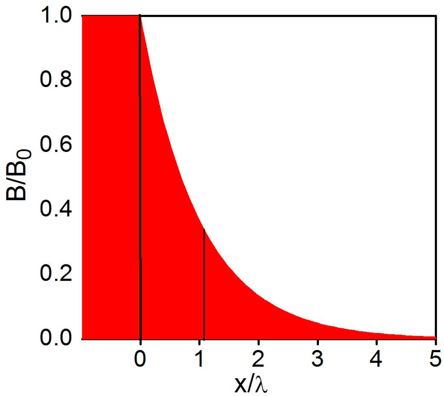
1.1. Superfluid Density

For clean metallic superconductors, $n_s\to n$ as $T\to 0$, where n is the concentration of carriers in the normal state. Non-local effects and other corrections lead to deviations in $\lambda$ from its London value. Hence, the superfluid density ${\rho }_s$ can be conveniently and more completely defined as:

$${\rho }_s\equiv 1/{\lambda }^2$$

(5)

which includes the effective mass and other corrections to the effective $n_s$, rather than the simpler definitions ${\rho }_s=n_s$ or ${\rho }_s=n_s/m^{*}$ that are sometimes used in the literature. ${\rho }_s$, a quantity of central importance in superconductivity, characterizes the phase stiffness of the condensate [5] and its effectiveness at screening out magnetic fields and feeds into expressions for the transition temperature (such as the Uemura relation $T_c\propto {\rho }_s\left(0\right)$ that applies to the underdoped cuprate superconductors [6,7,8]).

Traditionally, many common methods for obtaining ${\rho }_s$ do so by directly or indirectly measuring $\lambda$ through its effect on a superconducting sample’s magnetic-field profile and consequent magnetic susceptibility. This category includes methods such as reflection of spin-polarized slow neutrons [9], mutual inductance altered by an intervening superconducting film [10,11], changes in the self-inductance of a coil that is part of an LC resonating circuit [12,13], muon-spin rotation [14], magnetic force microscopy [15], microwave cavity resonance [16], and measurements of the lower critical field. These measurements are understandably affected if the material’s internal magnetic field is altered, for example by a large paramagnetic background as in the case of the Nd_2−xCe_xCuO₄ superconductor because of its Nd³⁺ magnetic moments.

Another approach to obtaining ${\rho }_s$ is by measuring the inertia of the superfluid (kinetic inductance) during its ballistic acceleration phase [17,18,19,20]. This method requires the sample to be patterned into very high aspect ratio meanders for the highest accuracy.

A measurement of $j_d$ provides an alternative to the above approaches for obtaining ${\rho }_s$. It requires a minimal amount of material (typically just a microbridge or nanobridge), does not require the complicated meander patterning needed for a kinetic-inductance measurement, and is unaffected by a material’s normal-state magnetism that affects inductive measurements of ${\rho }_s$ as discussed above. This immunity to material magnetism was used to good advantage for directly obtaining ${\rho }_s$ in the Nd_2−xCe_xCuO₄ superconductor for the first time [21]. Furthermore, unlike some of the methods for measuring $\lambda$ that do not provide an accurate absolute value but only provide the temperature variation $\lambda \left(T\right)/\lambda \left(0\right)$, $j_d$ does provide the absolute value of $\lambda$ and ${\rho }_s$ and can hence provide information on the total carrier concentration n.

1.2. Normal-State Resistivity

Another valuable byproduct of measuring $j_d$ is that it provides a direct measurement of the normal state resistivity ${\rho }_n$ for temperatures below $T_c$. One of the starting points in developing an understanding of any newly-discovered superconductor is to understand the underlying normal state: the type of carriers and their concentration, their band-related properties, and the relevant scattering mechanisms and rates. At low applied B and j, $\rho \left(T\right)$ drops precipitously below $T_c$, thereby obscuring how ${\rho }_n(T\ll T_c)$ would have behaved if the superconductivity had not set in. The most common method for measuring ${\rho }_n(T<T_c)$ utilizes high magnetic fields $B>B_{c2}$ to drive the system normal below $T_c$; however, this measurement is subject to magnetoresistance (typically $R\left(B\right)\ne$ const) and may require prohibitively high magnetic fields ($B_{c2}>100$ T for some superconductors).

One alternative is to use the core of a magnetic flux vortex as a window to the normal state. From Equation (1), a measurement of ${\rho }_f$ elucidates ${\rho }_n$ [22]. However, this extraction of ${\rho }_n$ requires interpretation and modeling, since Equation (1) usually holds only approximately except for very high driving forces, and the exact prefactor depends on the detailed regime of flux flow [23,24,25].

Current-induced depairing provides an especially clean method for destroying superconductivity and accessing ${\rho }_n(T\ll T_0)$. Like the method of applying $B>B_{c2}$ to drive the system normal, applying $j>j_d$ is also free of interpretation and modeling, unlike flux-flow dissipation measurements. On the other hand, unlike the potential errors in the $B_{c2}$-based measurement due to normal-state magnetoresistance, the $j_d$ method is immune to this issue because the normal-state electroresistance is quite negligible (i.e., $R\left(E\right)\simeq$ const) under the electric fields that arise at depairing conditions.

Thus, besides the investigation of interesting phenomena and regimes in superconductivity related directly to current-induced depairing itself, the study of $j_d$ provides information on the important parameters of the superconducting state such as ${\rho }_s\left(T\right)$ and ${\rho }_n\left(T\right)$.

2. Relationship between the Depairing Current and Other Parameters

In a microscopic theory such as the Bardeen–Cooper–Schrieffer (BCS) theory, experimental quantities are calculated from microscopic parameters such as the strength of the effective attractive interaction that leads to Cooper pair formation and the density of states at the Fermi level. Often, these microscopic parameters are not sufficiently well known. In the London and Ginzburg–Landau (GL) phenomenological theories, connections are made between the different observables from constraints based on thermodynamic principles and electrodynamical properties of the superconducting state, leading to an adequate estimation of the depairing current. These phenomenological formulations are described next [4,26].

2.1. London Formulation

The London theory [4,27] of superconductivity provides a description of the observed electrodynamical properties by supplementing the basic Maxwell equations by additional equations that constrain the possible behavior to reflect the two hallmarks of the superconducting state: perfect conductivity and the Meissner effect. Note that these properties hold only partially when vortices are present.

An ordinary metal (normal conductor) requires a driving electric field E to maintain a constant current against resistive losses. In the simple Drude picture, this produces Ohm’s law behavior, $j=\sigma E$, with a conductivity given by $\sigma =n{e}^2\tau /m^{*}$. A superconductor can carry a resistanceless current, and so, an electric field is not required for maintaining a persistent current. Instead, E in a perfectly-conducting state causes a ballistic acceleration of charge so that:

$$E=\left(\frac{m^{*}}{n_s{e}^2}\right)\frac{\partial j}{\partial t}$$

(6)

This is the first London equation, which reflects the dissipationless acceleration of the superfluid.

The second property that needs to be accounted for is the expulsion of magnetic flux by a superconductor. The magnetic field is exponentially screened from the interior following a spatial dependence:

$${\nabla }^{2}B=B/{\lambda }_L^2$$

(7)

Together with the Maxwell equation $\nabla \times B={\mu }_{0}j$, this implies the following condition between B and j:

$$B=-{\mu }_0{\lambda }_L^2(\nabla \times j)$$

(8)

This is the second London equation, which describes the property of a superconductor to exclude magnetic flux from its interior. Taken together with the Maxwell equation $\nabla \times E=-\partial B/\partial t$, Equations (6) and (8) yield the expression for ${\lambda }_L$ of Equation (4).

Besides the London equations themselves, a third ingredient needed for the estimation of $j_d$ in this framework is the thermodynamic critical field $B_c$ and its relationship to the Helmholtz free energy density f. When flux is expelled, the free energy density is raised by the amount $B^2/2{\mu }_0$. The critical flux expulsion energy (for the ideal case of a type-I superconductor with a non-demagnetizing geometry and dimensions large compared to the penetration depth) corresponds to the condition:

$$f_c=f_n-f_s=\frac{B_c^2}{2{\mu }_0}$$

(9)

where the L.H.S. of the equation represents the condensation energy density, which is the difference in free energy densities $f_n-f_s$ between the normal and superconducting states. $j_d$ represents the condition when the kinetic energy density equals the condensation energy density: $\frac{1}{2}{n}_s{m}^{*}{v}_s^2=\frac{m^{*}{j}_d^2}{2n_s{e}^2}=\frac{B_c^2}{2{\mu }_0}$, where $v_s$ is the superfluid speed. Substituting for ${\lambda }_L$ (Equation (4)) gives the London estimate for the depairing current density:

$$j_d\le \frac{B_c}{{\mu }_0{\lambda }_L}$$

(10)

The inequality reflects the fact that $n_s$ does not remain constant, but diminishes as j approaches $j_d$.

2.2. Ginzburg–Landau Formulation

There are situations where a system’s quantum wavefunction cannot be solved for by usual means because the Hamiltonian is unknown or not easily approximated. The GL formulation [28] is a clever construction that allows useful information and conclusions to be extracted in such a situation where one cannot solve the problem quantum mechanically. For describing macroscopic properties, such as $j_d$ that we are about to calculate, the GL theory is in fact more amenable than the microscopic theory [4,29].

The idea is to introduce a complex phenomenological order parameter (pseudo wavefunction) $\psi =\left|\psi \right|e^{i\phi }$ to represent the superconducting state. ${\left|\psi \left(r\right)\right|}^2$ is assumed to represent the order parameter $\Delta$ introduced earlier, and to approximate the local density of paired superconducting charge carriers (Cooper pairs), which in turn is half the density of superconducting electrons $n_s$.

The free energy density $f_s$ of the superconducting state is then expressed as a reasonable function of $\psi \left(r\right)$ plus other energy terms. A “solution” to $\psi \left(r\right)$ is now obtained by the minimization of free energy rather than through quantum mechanics. The unknown parameters of the theory are then solved in terms of measurable physical quantities, thereby providing constraints between the different quantities of the superconducting state.

Close to the phase boundary, ${\left|\psi \right|}^2$ is small, and so, $f_s$ can be expanded keeping the lowest two orders of ${\left|\psi \right|}^2$. First, let us consider the simplest situation where there are no currents, gradients in $\left|\psi \right|$, or magnetic fields present. Then, we have:

$$f_s=f_n+{\alpha \left|\psi \right|}^2+\frac{\beta }{2}{\left|\psi \right|}^4,$$

(11)

where $\alpha$ and $\beta$ are temperature-dependent coefficients whose values are to be determined in terms of measurable parameters. The coefficients can be determined as follows. First of all, for the solution of ${\left|\psi \right|}^2$ to be finite at the minimum free energy, $\beta$ must be positive. Second, for the solution of ${\left|\psi \right|}^2$ to be non-zero, $\alpha$ must be negative. Since ${\left|\psi \right|}^2$ vanishes above $T_c$, $\alpha$ must change its sign upon crossing $T_c$. The minimum in $f_s$ occurs at:

$${\left|\psi \right|}^2=-\alpha /\beta .$$

(12)

Substituting this back in Equation (11) and using the definition of $B_c$ (Equation (9)), Equation (12) can be written as:

$$f_c=\frac{B_c^2}{2{\mu }_0}=\frac{{\alpha }^2}{2\beta }$$

(13)

giving one of the connections between $\alpha$ and $\beta$ and a measurable quantity ($B_c$). A second connection can be obtained by noting that $n_s$ in Equation (4) can be replaced by $2{\left|\psi \right|}^2$, taking its equilibrium value from Equation (12):

$${\lambda }^2=\frac{m^{*}}{2{\mu }_0{\left|\psi \right|}^2{e}^2}=\frac{-\beta }{\alpha }\left(\frac{m^{*}}{2{\mu }_0{e}^2}\right)$$

(14)

Solving Equations (13) and (14) simultaneously gives the GL coefficients:

$$\alpha =-\frac{2e^2{B}_c^2{\lambda }^2}{m^{*}}\mathrm{and}\beta =\frac{4{\mu }_0{e}^4{B}_c^2{\lambda }^4}{m^{*2}}$$

(15)

Note that e and $m^{*}$ refer to single-carrier values and not pair values.

To calculate $j_d$, we include the effect of a current in Equation (11) by adding a kinetic energy term $\frac{1}{2}{n}_s{m}^{*}{v}_s^2={\left|\psi \right|}^2{m}^{*}{v}_s^2$ to it:

$$f_s=f_n+{\alpha \left|\psi \right|}^2+\frac{\beta }{2}{\left|\psi \right|}^4+{\left|\psi \right|}^2{m}^{*}{v}_s^2.$$

(16)

For zero j and $v_s$, we saw earlier (Equation (12)) that the equilibrium value of ${\left|\psi \right|}^2$ that minimizes the free energy is $|{\psi }_{j=0}{|}^2=-\alpha /\beta$. For a finite j and $v_s$, minimization of Equation (16) gives the value of ${\left|\psi \right|}^2$ when it is suppressed by a current:

$$|{\psi }_{j\ne 0}{|}^2=\frac{-\alpha }{\beta }\left(1-\frac{m^{*}{v}_s^2}{\left|\alpha \right|}\right)={\left|{\psi }_{j=0}\right|}^2\left(1-\frac{m^{*}{v}_s^2}{\left|\alpha \right|}\right)$$

(17)

The corresponding supercurrent density is then:

$$j=2e|{\psi }_{j\ne 0}{|}^2{v}_s=\frac{-2e\alpha }{\beta }\left(1-\frac{m^{*}{v}_s^2}{\left|\alpha \right|}\right)v_s$$

(18)

The maximum possible value of this expression can now be identified with $j_d$:

$$j_d\left(T\right)=\frac{-4e\alpha }{3\beta }{\left(\frac{\left|\alpha \right|}{3m^{*}}\right)}^{1/2}={\left(\frac{2}{3}\right)}^{3/2}\frac{B_c\left(T\right)}{{\mu }_0\lambda \left(T\right)}$$

(19)

where the GL-theory parameters were replaced by their expressions in terms of the physical measurables $B_c$ and $\lambda$ through Equation (15). As anticipated at the end of Equation (10) for the London derivation for $j_d$, that simpler estimate is indeed larger than this more rigorous GL derivation by the factor ${(3/2)}^{3/2}$ = 1.84.

The approximate temperature dependence of $j_d$ can be obtained by inserting the generic empirical temperature dependencies $B_c\left(T\right)\approx B_c\left(0\right)[1-{(T/T_c)}^2]$ and $\lambda \left(T\right)\approx \lambda \left(0\right)/\sqrt{[1-{(T/T_c)}^4]}$, giving:

$$j_d\left(T\right)\approx j_d\left(0\right){[1-{(T/T_c)}^2]}^{\frac{3}{2}}{[1+{(T/T_c)}^2]}^{\frac{1}{2}}$$

(20)

which close to $T_c$ reduces to:

$$j_d\left(T\right)\approx \sqrt{2}{j}_d\left(0\right){[1-{(T/T_c)}^2]}^{\frac{3}{2}}.$$

(21)

where $j_d\left(0\right)$ is given by Equation (19) by setting $T=0$ (for high scattering “dirty” superconductors, the $\sqrt{2}$ prefactor can be smaller or absent [29,30]).

Since $B_c$ is not an easy quantity to measure directly, the relation:

$$B_c=\sqrt{\frac{{\mathsf{\Phi }}_0{B}_{c2}}{4\pi {\lambda }^2}}$$

(22)

can be used along with Equation (19) to write the expression for $j_d$$\left(0\right)$:

$$j_d\left(0\right)=\sqrt{\frac{2{\mathsf{\Phi }}_0{B}_{c2}\left(0\right)}{27\pi {\mu }_0^2{\lambda }^4\left(0\right)}}$$

(23)

that has the more easily measurable $B_{c2}$. Since both $B_{c2}$ and $j_d$ can be obtained from transport measurements, this becomes a convenient way to obtain $\lambda$ and, hence, ${\rho }_s$.

2.3. Microscopic Formulations and Generalizations

Various authors have calculated $j_d\left(T\right)$ from a microscopic basis [29,31,32]. For arbitrary temperatures and mean free paths, one must use the Gorkov equations as the starting point. Kupriyanov and Lukichev [33] have derived $j_d\left(T\right)$ from the Eilenberger equations, which are a simplified version of the Gorkov equations. This derivation is beyond the scope of the present review, but a nice shortened version can be found in [30]. The microscopic calculation confirms the overall temperature dependence predicted by GL, and the two normalized curves differ only slightly from each other (e.g., see Figure 4 of [30]). Thus, the GL theory can be applied over the entire temperature range down to $T\ll T_c$. The previous equations relating $j_d$ to $B_c$ and $\lambda$ are expected to hold in the case of multiple bands and other gap symmetries, as long as one uses the actual empirical temperature dependencies of $B_c$ and $\lambda$, which account for modifications in these unconventional cases. This was experimentally demonstrated in the case of MgB₂ [26], which was recognized as a multi-gap superconductor tuned by strain and doping in the early part of this century; in fact, MgB₂ showed superconductivity near a Lifshitz transition as in iron-based superconductors [34,35,36].

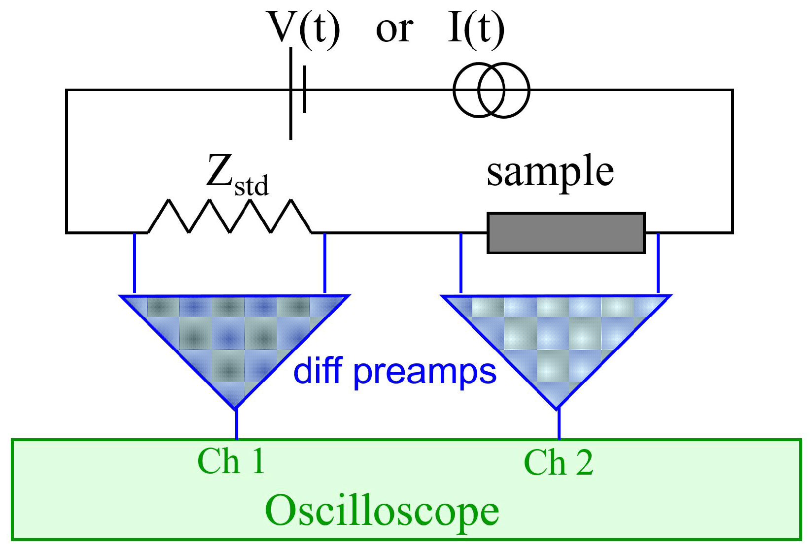
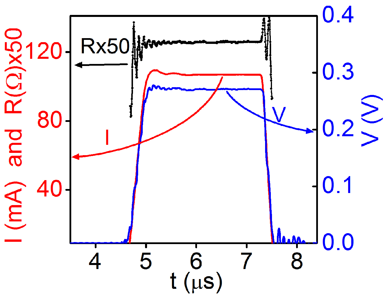
3. Pulsed Measurement Technique

Depairing current densities in superconductors is extremely high: on the order of $j_d$(T = 0) = ${10}^{11}$–${10}^{13}$ A/m². If the cross-section of the sample is even as narrow as just 1 mm², the current required would reach a value of $I=jA\sim {10}^6$ A. Such a magnitude of current would be exceedingly difficult to produce and control. There are three steps to overcoming this dilemma: (1) Fabricate samples with very narrow cross-sectional areas. This can be achieved by growing nanowires and nanorods or by depositing very thin films and using lithography to pattern narrow bridges (alternatively, the films can be deposited onto nanowires or carbon nanotubes). (2) The next step is by pulsing the current at very low duty cycles so that large values of I can be handled while reducing the time-averaged current and time-averaged power dissipation to manageable levels. (3) The last step is limiting the measurement of $j_d$ to the regime close to $T_c$. From Equation (21), it would seem that $j_d$ can be made arbitrarily small by making T very close to $T_c$; however, the $T-T_c$ distance needs to be large compared to the transition width for the measurement to be meaningful. Even for this near-$T_c$ measurement of $j_d$, the current usually will have to be pulsed to avoid significant sample heating. Furthermore, the near-$T_c$ measurement will only measure ${\rho }_s$ in that region, and its zero-T value will have to be extrapolated using theory. While this is better than nothing, it will not shed light on any abnormal temperature dependence of ${\rho }_s$ over the entire range, which could be of special interest if the superconductor has some exotic behavior.

Thus, the experimental ingredients needed to conduct a $j_d$ measurement are: a superconducting sample with a very narrow cross-section; a means to control the temperature, i.e., a cryostat; and a method for sourcing pulsed signals (current or voltage) and detecting the consequent complementary signal (voltage or current). There are numerous methods for sample fabrication, which vary widely with the different superconducting materials. Some deposition systems for preparing superconducting films can be bought off the shelf. Cryostats also represent standard equipment that can be bought off the shelf. The principal distinguishing the experimental capabilities of our work center on the pulsed electrical measurements. Therefore, the rest of the experimental section will be devoted to describing this unique measurement setup.

Figure 2 shows the overall configuration and functional schematic. The pulsed current/voltage source puts out a time-varying current and voltage. This signal flows through a standard impedance, usually a resistor $R_{std}$ (although an inductor is preferable in some situations) and the superconducting sample of resistance R that are in series. The initial signal can be taken directly from the output of a standard pulse generator (one of the models used was a Wavetek Model 801). These signal generators will typically have an output impedance of $Z_{out}=50\mathsf{\Omega }$. If a lower $Z_{out}$ is desirable (to allow for constant voltage control), the signal generator’s output can be passed through any standard buffer amplifier (e.g., a transistor-emitter-follower-based circuit, a power-operational-amplifier-based circuit, or an off-the-shelf audio amplifier). If a higher voltage than the signal generator’s output is desirable, its output can be passed through any standard voltage amplifier (fast high quality audio amplifiers can serve this purpose as well). Combining a higher voltage signal with a large series resistor (which can be the $R_{std}$ itself or an additional series resistor) can provide a relatively constant current. In general, the measurement will be in current-controlled or voltage-controlled mode depending on whether the combination of the final $Z_{out}$ (after the amplifier if any) plus $R_{std}$ is greater than or less than R. If the current needs to be held constant to a high accuracy (for example, if a series of R vs. T resistive transition curves needs to be traced out at various constant currents, as will be seen later), then it is better to follow the pulse generator with a transconductance amplifier, which converts the generator’s voltage pulse into a constant current pulse. The transconductance amplifier is able to hold the current constant by electronic circuity instead of needing an enormous series resistance. While conducting a pulsed current-voltage ($IV$) curve, which is usually done manually, it is preferable to have the voltage-controlled mode. The reason for this is that as the current and voltage are pushed higher, the sample’s resistance will increase, and at some point, the sample will be driven to normal as $j_d$ is exceeded. In constant-current mode, the power dissipation $P=I^{2}R$ rises as R rises, causing an increase in heating and a further rise in R. This can lead to a run-away condition, which can destroy the sample. On the other hand, the constant-voltage mode is self-stabilizing since in this case, $P=V^2/R$ decreases as R rises, thus reducing heating and controlling the situation.

Once the current pulse flows through the sample and $R_{std}$, the corresponding time-varying voltages, $V(t$) and $V_{std}\left(t\right)$, will be developed across them respectively. These must be observed and quantified using an oscilloscope. A digital storage oscilloscope (DSO) allows multiple pulses to be averaged. Since the signal is exactly repetitive, because the DSO is triggered off of the pulse generator’s sync signal, the averaging effectively suppresses random uncorrelated noise. As long as the sample condition (T, B, etc.) is stable, a very high number of averages can be taken to improve the signal-to-noise ratio (SNR) vastly. Coaxial cables with 50-Ohm characteristic impedance are used between all connection points, including the wiring within the cryostat. Where possible, the originating and/or terminating points at the ends of the cables need to have matching 50-Ohm values to avoid reflections. Multiple ground connections to the circuit must be avoided to prevent ground loops. This means the two channels of the DSO cannot be simultaneously connected to both the sample and $R_{std}$; either a differential instrumentation preamplifier (Princeton Applied Research and Stanford Research Systems are two brands that make instrumentation amplifiers) must be used between the DSO channels and the sample and $R_{std}$, or only one of the two must be measured at a time.

Figure 3 shows the pair of time-varying current $I\left(t\right)=V_{std}\left(t\right)/R_{std}$ and sample-voltage $V\left(t\right)$ signals that results. The topmost trace is the scaled calculated resistance $50R\left(t\right)=50V\left(t\right)/I\left(t\right)$. Note that the pulses reach constant plateaus after their initial transients. R, V, and I are defined by taking the plateau values of the individual quantities. The thermal rise in a sample because of Joule heating involves several processes: thermal diffusion occurs within the sample essentially instantaneously; on the time scale of nanoseconds, phonons transfer heat across the interface between the film and substrate; heat then diffuses within the substrate in a matter of microseconds and finally into the heat sink in milliseconds. For those processes that have time scales comparable to or longer than the pulse duration, there will be a visible rise in $V\left(t\right)$, causing the pulse to be distorted. Thus, as long as the $V\left(t\right)$ pulse is flat, slow causes of heating that influence the $V\left(t\right)$ shape can be assumed to be negligible. The work in [37] discusses a method to evaluate a sample’s thermal resistance for pulsed signals quantitatively.

Figure 4 shows an example [26] of a set of IV curves at various fixed temperatures (in zero magnetic field), where each data point represents a pulsed measurement (plateau values) as described above. As the temperature is increased, $j_d$ is reduced, and hence, the “jump” occurs at a lower value of I. Notice that the resistance (the V/I slope) jumps from zero (dissipationless superconducting state) to a constant finite value (normal-state) as the current crosses its depairing value. This is one direct way of obtaining ${\rho }_n$ below $T_c$. In this particular material, high impurity scattering dominates over electron-phonon scattering at all temperatures, leading to a relatively flat $\rho \left(T\right)$. A more interesting application of this technique for elucidating a variable $\rho \left(T\right)$ is described in a later section.

Figure 5a represents a set of pulsed constant-current $R\left(T\right)$ curves in zero magnetic field [38]. As the current is increased, the transition is progressively pushed down in temperature. Figure 5b plots these midpoint transition temperatures ($T_{c2}$) versus I, and they are seen to follow a $I^{2/3}$ law as per Equation (21). From this measured slope and Equation (21), one can estimate $j_d\left(0\right)$ without requiring the application of this enormous value of current. This is especially useful for systems (e.g., cuprate high-temperature superconductors) that have a very high $j_d\left(0\right)$ value.

Figure 6 shows the companion very low DC-current $R\left(T\right)$ curves at various constant B values. Here, the shift occurs because of the $B_{c2}\left(T\right)$ boundary; the current level is small enough for its depairing to be negligible. Unlike $j_d\left(T\right)$, $B_{c2}\left(T\right)$ has a linear dependence near $T_c$, and that slope can be related to $B_{c2}\left(0\right)$ through the WHH (Werthamer, Helfand, and Hohenberg) theory [39] and its variations [40] by relationships such as $B_{c2}\left(0\right)\simeq 0.7d{B}_{c2}/dT$.

The measurements represented by Figure 5 and Figure 6 together with Equation (23) are the key to obtaining ${\rho }_s$ through relatively straightforward transport measurements. We now look at one recent example of a current-induced depairing study of an exotic superconducting system.

4. Investigations in a Topological Insulator/Chalcogenide Interfacial Superconductor

4.1. Background

The interface between the Bi₂Te₃ topological insulator and the FeTe chalcogenide provides a fascinating 2D superconducting system, in which neither Bi₂Te₃, nor FeTe are superconducting by themselves [41]. While the exact origin of the superconductivity is not known, it has been suggested that the robust topological surfaces states may be doping the FeTe and suppressing the antiferromagnetism in a thin region close to the interface, thus inducing the observed 2D superconductivity. These surface states represent a conducting system with very high normal conductivity because of protection against time-reversal-invariant scattering mechanisms. Therefore, it is of great interest to understand the nature and origin of the charge carriers that underlie this interfacial superconductivity, and in particular, to see if the topologically-protected surface states might be a source of the normal carriers. The relevance of this question is broader than the specific system studied here, since it has been recently proposed that interfacial superconductivity may even play a role in cuprates: for example, in the interface located between charge density wave nanoscale puddles [42] and between oxygen-rich grains where the interface is made of a filamentary network with hyperbolic geometry [43,44]. We describe below how the current-induced depairing approach was used to answer these questions to elucidate the nature of the normal state in the Bi₂Te₃/FeTe system.

4.2. Samples and Experimental Information

The Bihe normal state in the /FeTe samples consisted of a ZnSe buffer layer (50 nm) deposited on a GaAs (001) semi-insulating substrate, followed by a deposition of 220 nm thick FeTe, which was then capped with a 20 nm-thick Bihe normal state in the layer. Upper-critical-field measurements [41] and vortex-explosion measurements [45] showed that the superconductivity occurred within an interfacial layer of thickness $d=7$ nm, which was much thinner than both the FeTe and Bihe normal state in the layers. Projection photolithography followed by argon-ion milling was used to pattern narrow microbridges optimized for the high current-density pulsed four-probe measurements. Two bridges were studied: Sample A with lateral dimensions of width $w=11.5$ μm and length $l=285$ μm and Sample B with $w=12$ μm and $l=285$ μm. The onset $T_c$ (defined as the intersection of the extrapolation of the normal-state portion and the extrapolation of the steep transition portion of the $R\left(T\right)$ curve) for both bridges, was 11.7 K. Details about sample preparation are provided in [41]. All measurements were made in zero applied magnetic field. While the very low reference curves at $I\le 60$ μA were measured using continuous DC signals, the main electrical transport measurements were made with pulsed signals. Contact resistances (<1 Ω) were much lower than the normal resistance $R_n$ of the bridge, and heat generated at contacts did not reach the bridge within the time duration t of each pulse, since the thermal diffusion distance ($\sqrt{Dt}\sim 10$ μm) was much shorter than the contact-to-bridge distance (>1 mm); here, D is the diffusion constant.

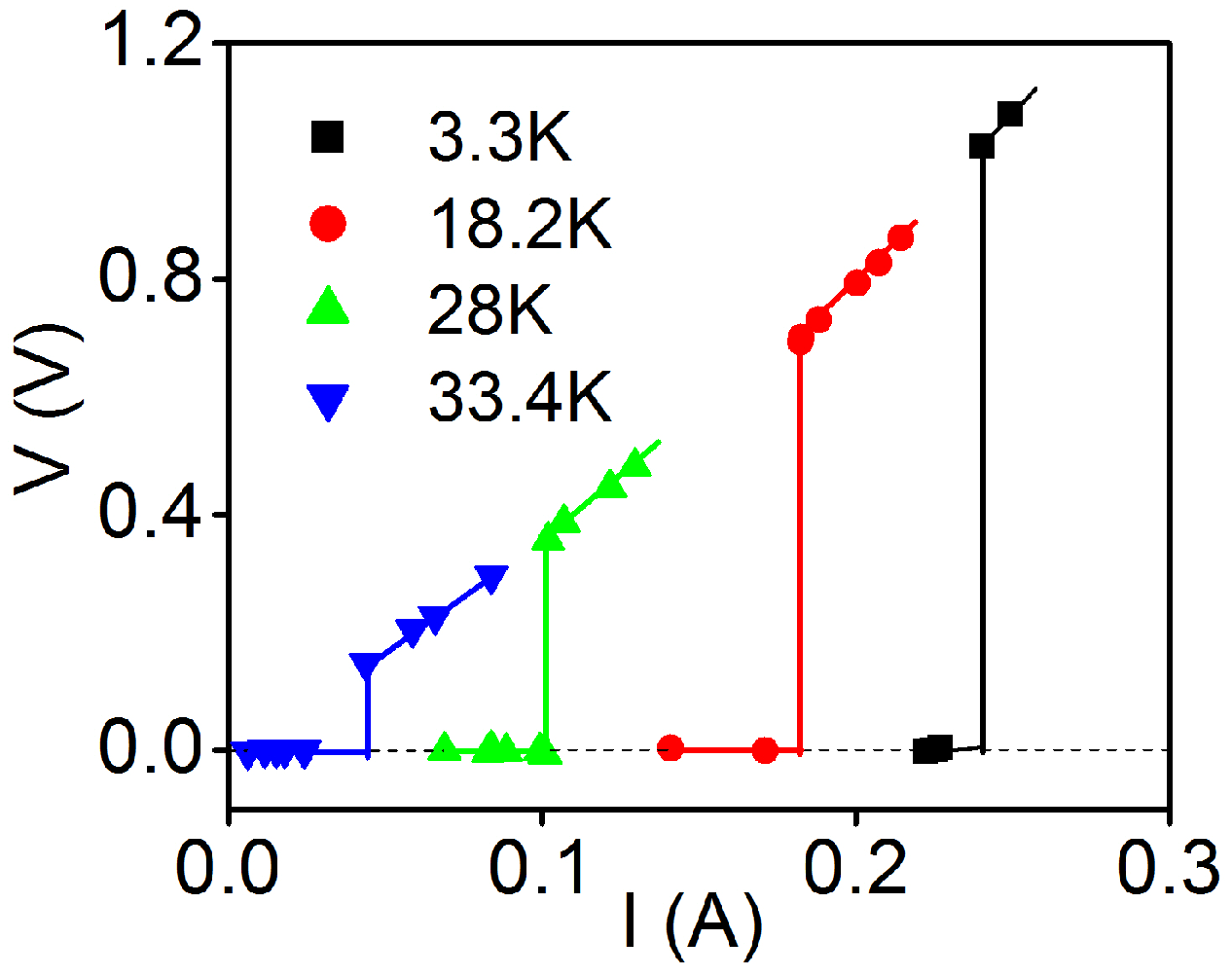
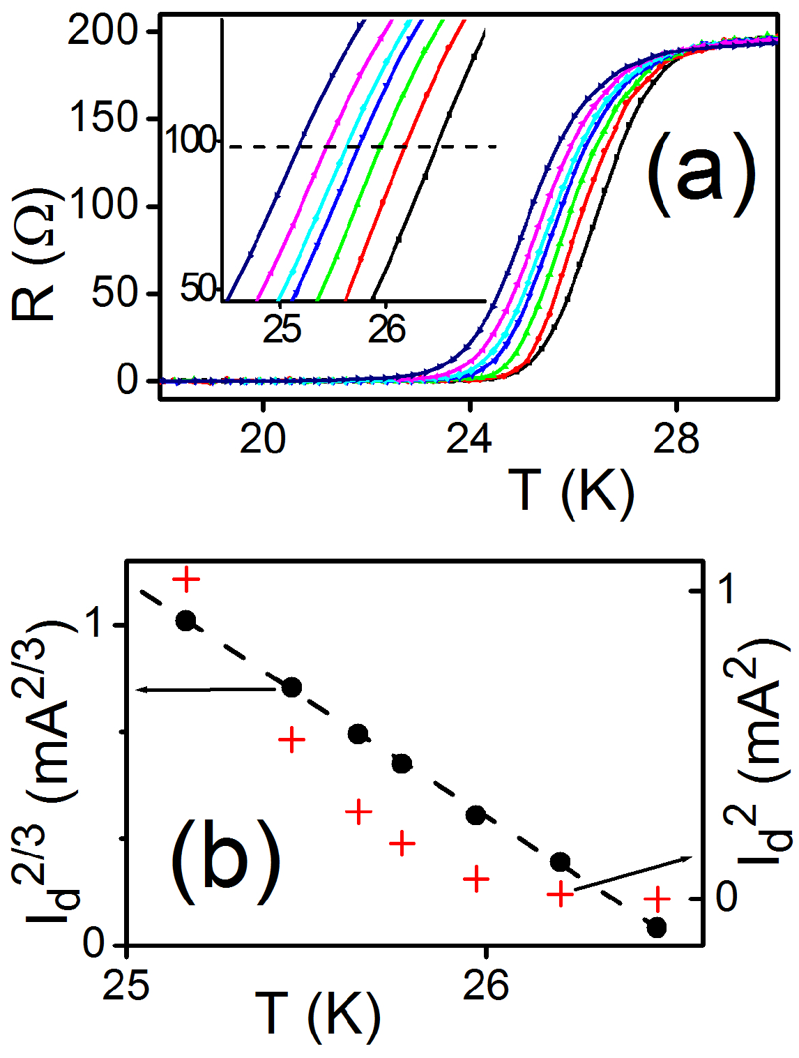
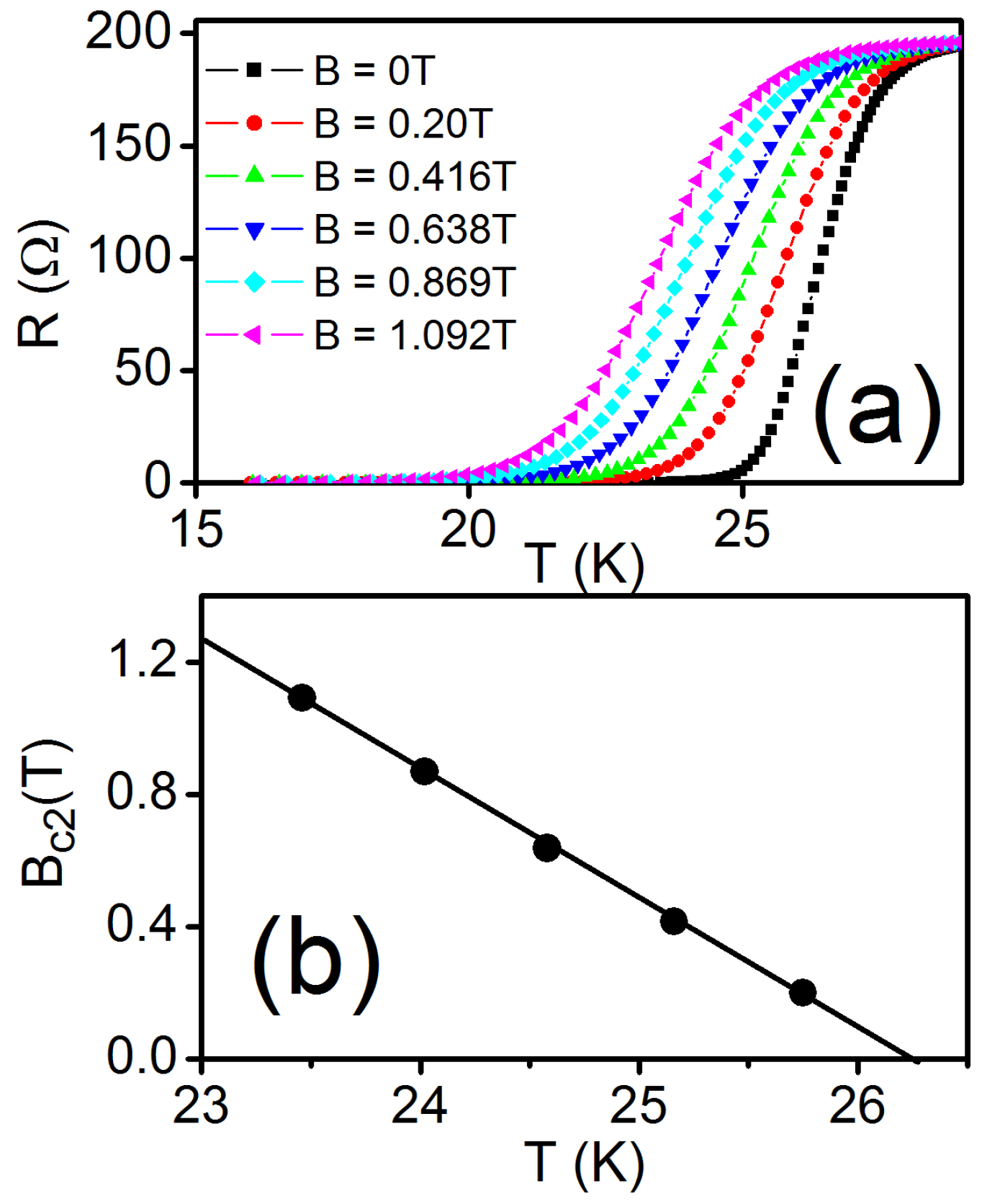
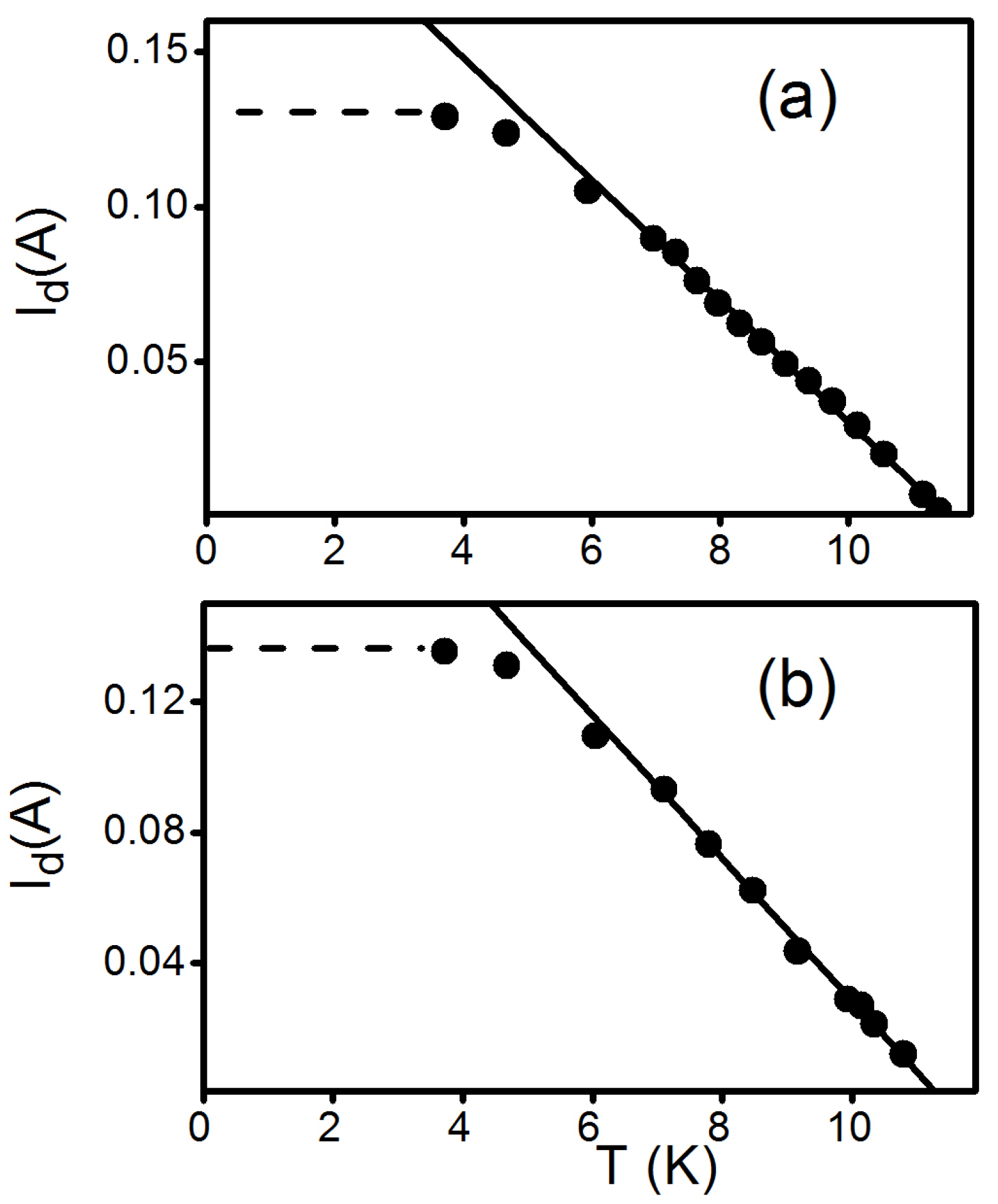
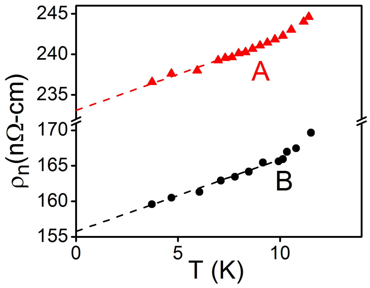
4.3. Results and Discussion

The normal-state resistivity ${\rho }_n\left(T\right)$ and depairing current density $j_d\left(T\right)$ in the Bi₂Te₃/FeTe samples were extracted over the entire temperature range [46], by driving the system normal with high pulsed currents using the methods described earlier and illustrated in Figure 4 and Figure 5. Figure 7 shows the raw depairing current results. The dashed horizontal lines in Panels (a) and (b) provide the values $I_d(T\to 0)\ge 0.131$ A and 0.136 A for Samples A and B, respectively.

In order to obtain more accurate intrinsic $j_d$ and ${\rho }_n$ of the 7 nm-thick superconducting interfacial layer itself, we needed to subtract the small parallel current through the normally conductive underlying FeTe layer. For this purpose, a separate measurement of pure FeTe deposited on ZnSe/GaAs, without the Bi₂Te₃ top layer, was conducted [46]. With this subtraction, the previous raw $I_d(T\to 0)$ values gave a corrected $j_d(T=0)$ of $1.5\times {10}^8$ A/cm² for both samples (which is a typical value: $j_d$ ranges ${10}^7$–${10}^9$ A/cm² for most superconductors), and the correction gave the intrinsic ${\rho }_n\left(T\right)$ for the two samples, as shown in Figure 8. This absolute value of ${\rho }_n(T\to 0)$∼200 nΩ cm represents an extraordinarily conductive normal state for a superconducting system, as most superconductors are poor conductors in the normal state. This information will be analyzed below within the framework of an anisotropic Ginzburg–Landau (GL) approach [46], to obtain information on the superfluid density, carrier concentration, and scattering rate, as well as their implications for the nature of the normal-state.

From the previously-published measurements of He et al. [41], we have the following orientation-dependent values of $B_{c2}$: perpendicular-to-interface $B_{c2}^{\perp }\left(0\right)\approx 17$ T and parallel-to-interface $B_{c2}^{\Vert }\left(0\right)\approx 40$ T. The corresponding coherence lengths from Equation (3) are: in-plane ${\xi }_{\Vert }\left(0\right)\approx 4.4$ nm and perpendicular ${\xi }_{\perp }\left(0\right)\approx 1.9$ nm. Using Equation (23) together with this $B_{c2}^{\perp }\left(0\right)$ and our measured in-plane $j_d^{\Vert }\left(0\right)$ gave ${\lambda }_{\Vert }\left(0\right)=124$ nm and a corresponding ${\rho }_s\left(0\right)=1/{\lambda }_{\Vert }^2\left(0\right)$. From ${\rho }_s\left(0\right)={\mu }_0{n}_s\left(0\right)e^2/m^{*}\approx {\mu }_{0}n{e}^2/m$ applicable in the clean limit at $T=0$, we get $n\approx 1.8\times {10}^{21}$ per cm³, approximating $m^{*}\approx m$. This effective single-band value of n evaluated above is similar to n characteristic of high temperature superconductors and about two orders of magnitude lower than n in highly-conductive metals such as copper.

The low value of n together with the very high normal conductivity implies a rather long scattering time $\tau$ and mean-free-path l. The Fermi wave number for this n computes to $k_F\left(3D\right)=m^{*}{v}_F/\hslash ={\left(3{\pi }^{2}n\right)}^{1/3}=3.8\times {10}^9$ m⁻¹ and $k_F\left(2D\right)={\left(2\pi nd\right)}^{1/2}=9.0\times {10}^9$ m⁻¹ in three and two dimensions, respectively. In both cases, the Fermi wavelength ${\lambda }_F=2\pi /k_F\ll d$, validating the continuum approximation for states along the perpendicular direction and justifying the anisotropic 3D treatment of the normal state. Then, from the Drude relationship $\rho \approx m/n{e}^2\tau$, we get $\tau \approx 10$ ps, which agrees well with the scattering rates ($\sim \hslash /0.05$ meV = 13 ps) measured by Pan et al. [47] using spin- and angle-resolved photoemission spectroscopy. Combining this value of $\tau$ with the Fermi velocity $v_F=\hslash k_F/m\approx 440$ km/s, we get $l=v_F\tau =4.2$ μm. The very long l, which well exceeds the superconducting layer thickness d, indicates that scattering from the faces that bound the superconducting layer was of a specular nature. This surprising dramatically low scattering indeed supports the possible role of the topological surface states in the formation of the normal state that underlies this exotic interfacial superconducting system.

5. Concluding Remarks

Fast pulsed signals of short duration and low duty cycle make it possible to study transport behavior in superconductors at extreme current densities, power densities, and electric fields. In this article, we focused on the use of this technique in the measurement of one of the fundamental critical parameters of the superconducting state, the depairing current $j_d$. It was shown how through $j_d$, one can obtain information on various other key parameters of the superconducting state, in particular the penetration depth and consequent superfluid density, which cast light on the normal state. As an example and illustration of this procedure, we described a recent study of the superconducting system formed at the interface between a topological insulator and a chalcogenide. We hope that the information provided here will encourage other groups to utilize this approach.

References

1. Onnes, K.H. Further experiments with liquid helium. C. On the change of electric resistance of pure metals at very low temperatures, etc. IV. The resistance of pure mercury at helium temperatures. In Through Measurement to Knowledge; Springer: Dordrecht, The Netherlands, 1911; pp. 261–263. [Google Scholar] [CrossRef]
2. Somayazulu, M.; Ahart, M.; Mishra, A.K.; Geballe, Z.M.; Baldini, M.; Meng, Y.; Struzhkin, V.V.; Hemley, R.J. Evidence for Superconductivity above 260 K in Lanthanum Superhydride at Megabar Pressures. Phys. Rev. Lett. 2019, 122, 027001–027004. [Google Scholar] [CrossRef] [PubMed]
3. Drozdov, A.P.; Kong, P.P.; Minkov, V.S.; Besedin, S.P.; Kuzovnikov, M.A.; Mozaffari, S.; Balicas, L.; Balakirev, F.; Graf, D.; Prakapenka, V.B.; et al. Superconductivity at 250 K in lanthanum hydride under high pressures. Nature 2019, 569, 528–531. [Google Scholar] [CrossRef] [PubMed] [Green Version]
4. Tinkham, M. Introduction to Superconductivity, 2nd ed.; Dover Publications: Mineola, NY, USA, 2004; ISBN-10: 0486435032; ISBN-13: 978-0486435039. [Google Scholar]
5. Emery, V.J.; Kivelson, S.A. Importance of phase fluctuations in superconductors with small superfluid density. Nature 1995, 374, 434–437. [Google Scholar] [CrossRef]
6. Uemura, Y.J.; Luke, G.M.; Sternlieb, B.J.; Brewer, J.H.; Carolan, J.F.; Hardy, W.N.; Kadono, R.; Kempton, J.R.; Kiefl, R.F.; Kreitzman, S.R.; et al. Universal Correlations between Tc and ns/m* (Carrier Density over Effective Mass) in High-Tc Cuprate Superconductors. Phys. Rev. Lett. 1989, 62, 2317–2320. [Google Scholar] [CrossRef] [PubMed]
7. Uemura, Y.J.; Le, L.P.; Luke, G.M.; Sternlieb, B.J.; Wu, W.D.; Brewer, J.H.; Riseman, T.M.; Seaman, C.L.; Maple, M.B.; Ishikawa, M.; et al. Basic similarities among cuprate, bismuthate, organic, Chevrel-phase, and heavy-fermion superconductors shown by penetration-depth measurements. Phys. Rev. Lett. 1991, 66, 2665–2668. [Google Scholar] [CrossRef] [PubMed]
8. Hardy, W.N.; Bonn, D.A.; Morgan, D.C.; Liang, R.; Zhang, K. Precision measurements of the temperature dependence of λ in Y1Ba2Cu3O7: Strong evidence for nodes in the gap function. Phys. Rev. Lett. 1993, 70, 3999–4002. [Google Scholar] [CrossRef] [PubMed]
9. Felcher, G.P.; Kampwirth, R.T.; Gray, K.E.; Felici, R. Polarized-Neutron Reflections: A New Technique Used to Measure the Magnetic Field Penetration Depth in Superconducting Niobium. Phys. Rev. Lett. 1984, 52, 1539–1542. [Google Scholar] [CrossRef]
10. Claassen, J.H.; Evetts, J.E.; Somekh, R.E.; Barber, Z.H. Observation of the superconducting proximity effect from kinetic-inductance measurements. Phys. Rev. B 1991, 44, 9605–9608. [Google Scholar] [CrossRef]
11. Yong, J.; Lee, S.; Jiang, J.; Bark, C.W.; Weiss, J.D.; Hellstrom, E.E.; Larbalestier, D.C.; Eom, C.B.; Lemberger, T.R. Superfluid density measurements of Ba(CoxFe1−x)2As2 films near optimal doping. Phys. Rev. B 2011, 83, 104510–104514. [Google Scholar] [CrossRef]
12. Boghosian, C.; Meyer, H.; Rives, J.E. Density, Coefficient of Thermal Expansion, and Entropy of Compression of Liquid Helium-3 under Pressure below 1.2 K. Phys. Rev. 1966, 146, 110–119. [Google Scholar] [CrossRef]
13. Van Degrift, C.T. Tunnel diode oscillator for 0.001 ppm measurements at low temperatures. Rev. Sci. Instr. 1975, 46, 599. [Google Scholar] [CrossRef]
14. Sonier, J.E. Muon spin rotation studies of electronic excitations and magnetism in the vortex cores of superconductors. Rep. Prog. Phys. 2007, 70, 1717–1756. [Google Scholar] [CrossRef]
15. Luan, L.; Auslaender, O.M.; Lippman, T.M.; Hicks, C.W.; Kalisky, B.; Chu, J.-H.; Analytis, J.G.; Fisher, I.R.; Kirtley, J.R.; Moler, K.A. Local measurement of the penetration depth in the pnictide superconductor Ba(Fe0.95Co0.05)2As2. Phys. Rev. B 2010, 81, 100501–100504. [Google Scholar] [CrossRef]
16. Shibauchi, T.; Kitano, H.; Uchinokura, K.; Maeda, A.; Kimura, T.; Kishio, K. Anisotropic penetration depth in La2-xSrxCuO4. Phys. Rev. Lett. 1994, 72, 2263–2266. [Google Scholar] [CrossRef]
17. Lee, J.Y.Y.; Lemberger, T.R. Penetration depth λ(T) of Y1Ba2Cu3O7 films determined from the kinetic inductance. Appl. Phys. Lett. 1993, 62, 2419–2421. [Google Scholar] [CrossRef]
18. Saracila, G.F.; Kunchur, M.N. Ballistic acceleration of a supercurrent in a superconductor. Phys. Rev. Lett. 2009, 102, 077001–077004. [Google Scholar] [CrossRef] [PubMed]
19. Diener, P.; Leduc, H.G.; Yates, S.J. Design and Testing of Kinetic Inductance Detectors Made of Titanium Nitride. J. Low Temp. Phys. 2012, 167, 305–310. [Google Scholar] [CrossRef] [Green Version]
20. Jochem, B. Kinetic Inductance Detectors. J. Low Temp. Phys. 2012, 167, 292–304. [Google Scholar]
21. Kunchur, M.N.; Dean, C.; Liang, M.; Moghaddam, N.S.; Guarino, A.; Nigro, A.; Grimaldi, G.; Leo, A. Depairing current density of Nd2−xCexCuO4 superconducting films. Physica C 2013, 495, 66–68. [Google Scholar] [CrossRef]
22. Kunchur, M.N.; Ivlev, B.I.; Christen, D.K.; Phillips, J.M. Metallic Normal State of Y1Ba2Cu3O7. Phys. Rev. Lett. 2000, 84, 5204–5207. [Google Scholar] [CrossRef] [PubMed]
23. Larkin, A.I.; Ovchinnikov, Y.U.N. Nonlinear conductivity of superconductors in the mixed state. Sov. Phys.—JETP 1976, 41, 960–965. [Google Scholar]
24. Blatter, G.; Feigel’man, M.V.; Mikhail, V.B.; Larkin, A.I.; Valerii, V.M. Vortices in high-temperature superconductors. Rev. Mod. Phys. 1994, 66, 1125–1388. [Google Scholar] [CrossRef]
25. Kunchur, M.N. Unstable flux flow due to heated electrons in superconducting films. Phys. Rev. Lett. 2002, 89, 137005–137008. [Google Scholar] [CrossRef] [PubMed]
26. Kunchur, M.N. Current-induced pair breaking in Magnesium Diboride. J. Phys. Condens. Matter. 2004, 16, R1183–R1204. [Google Scholar] [CrossRef]
27. London, F.; London, H. The electromagnetic equations of the supraconductor. Proc. Roy. Soc. 1935, A149, 71–88. [Google Scholar] [CrossRef]
28. Ginzburg, V.L.; Landau, L.D. On the Theory of superconductivity. Zh. Eksperim. Teor. Fiz. 1950, 20, 1064–1082. [Google Scholar]
29. Bardeen, J. Critical Fields and Currents in Superconductors. Rev. Mod. Phys. 1962, 34, 667–681. [Google Scholar] [CrossRef]
30. Romijn, J.; Klapwijk, T.M.; Renne, M.J.; Mooij, J.E. Critical pair-breaking current in superconducting aluminum strips far below Tc. Phys. Rev. B 1982, 26, 3648–3655. [Google Scholar] [CrossRef]
31. Maki, K. On Persistent Currents in a Superconducting Alloy. II. Progr. Theor. Phys. 1963, 29, 333–340. [Google Scholar] [CrossRef] [Green Version]
32. Ovchinnikov, Y.U.N. Critical current of thin films for diffuse reflection from the walls. Sov. Phys.—JETP 1969, 29, 853–860. [Google Scholar]
33. Kupriyanov, M.Y.; Lukichev, V.F. Temperature dependence of pair-breaking current in superconductors. Sov. J. Low Temp. Phys. 1980, 6, 210. [Google Scholar]
34. Bauer, E.; Paul, C.; Berger, S.; Majumdar, S.; Michor, H.; Giovannini, M.; Saccone, A.; Bianconi, A. Thermal conductivity of superconducting MgB2. J. Phys. Condens. Matter 2001, 13, L487–L493. [Google Scholar] [CrossRef]
35. Agrestini, S.; Metallo, C.; Filippi, M.; Simonelli, L.; Campi, G.; Sanipoli, C.; Liarokapis, E.; De Negri, S.; Giovannini, M.; Saccone, A.; et al. Substitution of Sc for Mg in MgB2: Effects on transition temperature and Kohn anomaly. Phys. Rev. B 2004, 70, 134514–134518. [Google Scholar] [CrossRef]
36. Kagan, M.Y.; Bianconi, A. Fermi-Bose Mixtures and BCS-BEC Crossover in High-Tc Superconductors. Condens. Matter 2019, 4, 51. [Google Scholar] [CrossRef]
37. Kunchur, M.N.; Christen, D.K.; Klabunde, C.E.; Phillips, J.M. Pair-breaking effect of high current densities on the superconducting transition in Y1Ba2Cu3O7. Phys. Rev. Lett. 1994, 72, 752–775. [Google Scholar] [CrossRef]
38. Liang, M.; Kunchur, M.N.; Fruchter, L.; Li, Z.Z. Depairing current density of infinite-layer Sr1−xLaxCuO2 superconducting films. Physica C 2013, 492, 178–180. [Google Scholar] [CrossRef]
39. Werthamer, N.R.; Helfand, E.; Hohenberg, P.C. Temperature and Purity Dependence of the Superconducting Critical Field, Hc2. III. Electron Spin and Spin-Orbit Effects. Phys. Rev. 1966, 147, 295–302. [Google Scholar] [CrossRef]
40. Gurevich, A. Enhancement of the upper critical field by nonmagnetic impurities in dirty two-gap superconductors. Phys. Rev. B 2003, 67, 184515–184527. [Google Scholar] [CrossRef]
41. He, Q.L.; Liu, H.; He, M.; Lai, Y.H.; He, H.; Wang, G.; Law, K.T.; Lortz, R.; Wang, J.; Sou, I.K. Two-dimensional superconductivity at the interface of a Bi2Te3/FeTe heterostructure. Nat. Commun. 2014, 5, 4247–4254. [Google Scholar] [CrossRef]
42. Campi, G.; Bianconi, A.; Poccia, N.; Bianconi, G.; Barba, L.; Arrighetti, G.; Innocenti, D.; Karpinski, J.; Zhigadlo, N.D.; Kazakov, S.M.; et al. Inhomogeneity of charge-density-wave order and quenched disorder in a high-Tc superconductor. Nature 2015, 525, 359–362. [Google Scholar] [CrossRef] [PubMed]
43. Jarlborg, T.; Bianconi, A. Multiple Electronic Components and Lifshitz Transitions by Oxygen Wires Formation in Layered Cuprates and Nickelates. Condens. Matter 2019, 4, 15. [Google Scholar] [CrossRef]
44. Campi, G.; Bianconi, A. High Temperature superconductivity in a hyperbolic geometry of complex matter from nanoscale to mesoscopic scale. J. Supercond. Nov. Magn. 2016, 29, 627–631. [Google Scholar] [CrossRef]
45. Dean, C.L.; Kunchur, M.N.; He, Q.L.; Liu, H.; Wang, J.; Lortz, R.; Sou, I.K. Current driven vortex-antivortex pair breaking and vortex explosion in the Bi2Te3/FeTe interfacial superconductor. Physica C 2016, 527, 46–49. [Google Scholar] [CrossRef]
46. Dean, C.L.; Kunchur, M.N.; He, Q.L.; Liu, H.; Wang, J.; Lortz, R.; Sou, I.K. Current-induced depairing in the Bi2Te3/FeTe interfacial superconductor. Phys. Rev. B 2015, 92, 094502–094506. [Google Scholar] [CrossRef]
47. Pan, Z.-H.; Fedorov, A.V.; Gerdner, D.; Lee, Y.S.; Chu, S.; Valla, T. Measurement of an Exceptionally Weak Electron-Phonon Coupling on the Surface of the Topological Insulator Bi2Se3 Using Angle-Resolved Photoemission Spectroscopy. Phys. Rev. Lett. 2012, 108, 187001–187005. [Google Scholar] [CrossRef]
Figure 1. An externally-applied magnetic field B 0 is screened from the interior of a superconductor in the Meissner state over a characteristic length scale, which is the magnetic-field penetration depth λ : B B 0 e x / λ . The circulating screening current is of roughly the depairing magnitude j d , so that λ 1 / j d .
Condensedmatter 04 00054 g001
Figure 2. The overall configuration and functional schematic of the pulsed-signal measurement system. The differential preamplifiers (diff preamps) convert the time-varying potential differences across standard impedance ( Z s t d ) and the sample, V s t d ( t ) and V ( t ) respectively, into ground referenced single-ended signals that can be fed to the inputs of a digital storage oscilloscope.
Condensedmatter 04 00054 g002
Figure 3. The measured oscilloscope traces of the sample voltage V ( t ) , current I ( t ) = V s t d ( t ) / R s t d , and scaled calculated resistance 50 R ( t ) = 50 V ( t ) / I ( t ) for an MgB2 bridge at 42 K (normal state just above T c ). The resistance rises from 10%–90% of its final value in about 50 ns (adapted from Reference [26]).
Condensedmatter 04 00054 g003
Figure 4. Current-voltage curves in a MgB2 bridge at various fixed temperatures. As the temperature is increased, j d is reduced, and hence, the “jump” occurs at a lower value of I. The sloped portions above each jump represent the normal-state resistance R n = Δ V / Δ I (adapted from from Reference [26]).
Condensedmatter 04 00054 g004
Figure 5. (a) Resistive transitions in a Sr1−xLaxCuO2 superconducting film bridge in zero magnetic field at various transport current values (right to left): 12.9, 132, 258, 426, 533, 721, and 1020 μA. The lowest current is continuous DC; the remaining currents are pulsed. The inset shows a magnified view of the midpoint region. (b) Left axis (circle symbols): two-thirds power of the depairing current versus the midpoint transition temperature corresponding to the depairing law. Right axis (plus symbols): square of the depairing current versus the midpoint transition temperature corresponding to Joule heating (adapted from Reference [38]).
Condensedmatter 04 00054 g005
Figure 6. (a) Resistive transitions of a Sr1−xLaxCuO2 superconducting film bridge at a constant current of I = 13 μA in various perpendicular magnetic field values as indicated in the key. (b) Upper critical magnetic field versus the midpoint transition temperature, extracted from the curves in (a) (adapted from Reference [38]).
Condensedmatter 04 00054 g006
Figure 7. Raw depairing current versus temperature for Bi2Te3/FeTe bridges: (a) Sample A and (b) Sample B. The dashed horizontal lines provide the values I d ( T 0 ) 0.131 A and 0.136 A for Samples A and B, respectively (adapted from Reference [46]).
Condensedmatter 04 00054 g007
Figure 8. Intrinsic normal-state resistivity of Bi2Te3/FeTe interfacial superconducting bridges, Samples A and B (adapted from Reference [46]).
Condensedmatter 04 00054 g008