1. Introduction
The capability of preparing and manipulating with high precision the state of a quantum system is essential for the study of quantum phenomena, both for the investigation of fundamental aspects and for the development of technological applications. One of the most interesting control methodologies relies on a fundamental result of Quantum Mechanics, namely the adiabatic theorem [
1]. This states that, given a time-dependent Hamiltonian, if the rate of the time evolution is sufficiently slow and there are no level crossings, then a system initially in an instantaneous eigenstate always remains in the corresponding instantaneous eigenstate at future times.
Although the adiabatic method is simple and robust by construction, for practical high-precision applications it often requires too long total evolution timescales, which are ultimately limited by dissipation and decoherence effects. For this reason, many strategies have been recently proposed for speeding up the quantum adiabatic dynamics, which are referred to as “shortcuts to adiabaticity” [
2]. These methods can produce the desired evolution exactly in arbitrarily short time, provided one is able to implement sufficiently strong control fields. However, the implementation of the accelerated protocol is often experimentally challenging. This is so since it typically requires time-dependent tuning of matrix elements which are not controllable in the original Hamiltonian [
2,
3], therefore demanding new resources and modifications of the experimental setup. Indeed, experimental proofs have been limited to few level systems and typically needed adaptations [
4,
5,
6,
7]. The problem can be circumvented by working in carefully selected interaction pictures and relaxing the constraint of following the adiabatic path at all times, i.e., by asking the evolution to match the adiabatic eigenstates only at the beginning and at the end of the protocol, see e.g., [
8,
9,
10]. This, however, results in a completely nonadiabatic method, thus arguably dropping the advantage of using adiabatic strategies.
Recently, it was shown that it is possible to achieve both effective instantaneous following of the adiabatic states and no necessity to control new matrix elements at the same time [
3]. This can be done by introducing fast oscillations in the parameters of the initial Hamiltonian which mimic the action of a full shortcut-to-adiabaticity Hamiltonian. Therefore, the necessity of new control knobs is traded for a high degree of controllability of those initially available and for an approximate rather than exact driving. This methodology has been theoretically exemplified in a precise circuit quantum electrodynamics (QED) experimental context in Ref. [
11], where the experimental realizability is discussed in detail.
An interesting feature recognized in previous work [
3,
11] is that this scheme requires precise phase relations between oscillations in different Hamiltonian matrix elements, which may not be easily guaranteed experimentally. Nonetheless, it was also noticed that small phase offsets could interestingly lead to an unpredicted improvement of the method. For this reason, in this work we elaborate in more detail on this phenomenon, studying how small biases in the relative phases of the control fields affect the performance of the protocol. We confirm that improvements can be obtained and we explain their origin in relation to the procedure for constructing the accelerating control fields. This new understanding allows us to speculate on the potential use of the phases of the control elements as additional parameters for optimizing the control method, also opening a connection with optimal control theory.
After reviewing the general method in
Section 2, we derive general system-independent expressions for the corrections to the final fidelity in
Section 3, which are then applied to the case study of a two-level system in
Section 4, connecting our results to previous work. In particular, it is explained that, in some cases, small phase shifts can be exploited to improve the control method without adding higher harmonics to the oscillating control functions. Our central result is Equation (
26) highlighting the role of the phase biases on the efficiency of the protocol. In
Section 5, it is then shown numerically that these mechanisms are present also in multilevel systems, by considering the case of a sped-up adiabatic protocol which produces entanglement between two qubits dispersively coupled to a resonator [
11].
4. Effect of Phase Shifts: Two-Level System
Using the general expressions reported in
Section 3, we study in this section the effects of phase shifts
in the control functions in a simple yet important scenario, namely that of a two-level system. In particular, the case of a two-level avoided crossing problem is considered in detail, being this a fundamental phenomenon where non-adiabaticity mechanisms become of paramount importance [
15]. An avoided crossing occurs when two levels whose energy difference is varied would cross if uncoupled, but, if they are coupled instead, they repel each other after reaching a minimal gap. This phenomenon was first described theoretically by Landau [
16], Zener [
17] and Majorana [
18], and has been studied thoroughly in a variety of experiments, see e.g., [
19,
20,
21,
22,
23]. Many complex nonadiabatic phenomena can also be reformulated by means of multiple single-avoided-crossing scenarios [
15,
24,
25,
26,
27]. Our aim is to show that slight phase offsets
can lead to an improvement of the fast adiabatic method based on fast oscillations discussed in the previous sections, and to explain this effect.
Let
be the Pauli matrices. Let us consider a two-state problem (
) with initial Hamiltonian
with
(
). That is, we assume that
H is controllable only along the
and
directions, while the
direction is not directly available due to experimental constraints. For instance, this can happen in planar superconducting circuits such as the transmon [
28] where it is not easy to control both real and imaginary parts of the couplings between bare levels [
7]. Note that the Hamiltonian
is real-valued, and we are thus in the case of
Section 3.3. The correcting Hamiltonian
, being a linear combination of the same control matrices
and
, can be written in the form
with
. As it has been suggested in Ref. [
3] a first-order cancellation method can be achieved by choosing control functions of the form
and
and this will be explained in more detail in the following. Here, since we want to study “dephasing” effects between the control fields, we allow for the presence of phase offsets
and
by taking
This choice, relative to Equation (
3), implies that only the fundamental frequency is present,
, and it moreover holds that
,
while
.
In order to compute an expression for the infidelity of Equation (
18) to the first two orders (
and
), one can use Equation (11). Moreover, one can use the exact expressions for the eigenvectors of
, which, since
is real-valued, can be written in the parametrized form
with
the azimuthal angle between
and the
z axis. In this way, one determines, using Equation (11),
where we have introduced the relative phase
, the matrices
and the nonadiabatic coupling
. The latter can be computed from the expressions in Equation (
20) to be
Thus, the first constraint equation,
, is
If one was not aware of the presence of the phase offset
, a solution for
could be taken to be
as was done in Ref. [
3]. This would be a good choice unless
was not a smooth function, in which case different solutions may be more convenient. Insertion of Equation (
22) into Equation (
18) gives the infidelity at the end of one time step
T. Assuming that the system is initially in the ground state,
, the result is
With this expression at hand, the effect of phase shifts in the initial control functions can now be discussed. For very small
T, one can focus on the first order,
, in Equation (
26). This determines the general behaviour; the infidelity oscillates for varying
with a period of
, reaching the maximum value for
,
—that is, when the oscillating part of the control functions of Equation (19) are in perfect phase match. On the other hand, the first order term is minimum for
, i.e., for control function with totally off-phase oscillating part as chosen in Equation (
19). Interestingly, the first order term turns out to be perfectly symmetric with respect to sign of
, so, if higher-order terms are neglected, no benefit can come for the presence of phase offsets, since in such a case it always holds that
.
Although the first term of the expansion of Equation (
26) determines the global behaviour of
, more details can be obtained by inspecting the second term, of order
. First of all, one can see that this is no more symmetric with respect to the sign of
, in general. In fact, a term
appears, breaking the symmetry unless
. This asymmetry has important consequences on the efficiency of the method; indeed, for certain values of
the infidelity can be become smaller than
due to a compensation of the terms in Equation (
26), leading eventually to an improvement of the fidelity.
Secondly, the term depends explicitly on and , so when this term becomes relevant the infidelity does not depend any more on the relative phase only. This means that, even once the relative phase is fixed, one may be able to tune and so to further minimize .
Thirdly, the
term depends also on the choice of
A and
B as solutions of the constraint Equation (
24). This induces a dependence on the choice of the adiabatic sweep function, via the nonadiabatic coupling
.
As a final remark, it must be noted that, for very small
, no information can in general be obtained from Equation (
26) if
enters a regime in which its magnitude is comparable with that of
T. In this case, in fact, Equation (
26) would no longer be a valid expansion, and more terms would need to be considered.
In order to corroborate the previous observations, we treat a specific example in the following section.
4.1. Application: Avoided Level Crossing
The standard scenario where nonadiabatic effects become of great importance is when an avoided crossing of energy levels occurs. A simple model to describe this phenomenon is to consider a two-level Hamiltonian of the form
with
constant in time while
is a sweep function such that
—that is, such that in absence of the coupling
the levels would cross at
. Depending on the rate of the sweep, which determines the speed of the evolution, adiabaticity may be satisfied or violated. The simplest choice for
is a linear sweep
, as proposed by Landau, Zener and Majorana [
15,
16,
17,
18]. For this case, an exact solution of the Schrödinger equation for
t going from
to
can be computed, for the system starting in the ground state, giving an asymptotic probability at time
that the system has jumped to the excited state. This is exponentially small in a certain adiabatic parameter which quantifies the speed of the evolution—namely
with
. In practical finite-time problems though, more refined choices for
are much preferable if one wants to achieve the best fidelity at the end of the sweep in a certain total time (while always remaining as close as possible to true adiabaticity, i.e., to being in an instantaneous eigenstate). For this reason, here we will work with the specific choice
with
where
is the initial energy gap,
is the total duration time of the sweep, and
. This kind of sweep function was introduced in Ref. [
11], following general recipes from Refs. [
29,
30], and guarantees that the instantaneous rate of the evolution satisfies an instantaneous adiabatic condition for all times.
Using the expressions (
19) and (
25), a correcting Hamiltonian for this problem is
with
.
Introducing the dimensionless quantities
and rescaling the physical time like
,
, the Schrödinger equation can be written in the dimensionless form:
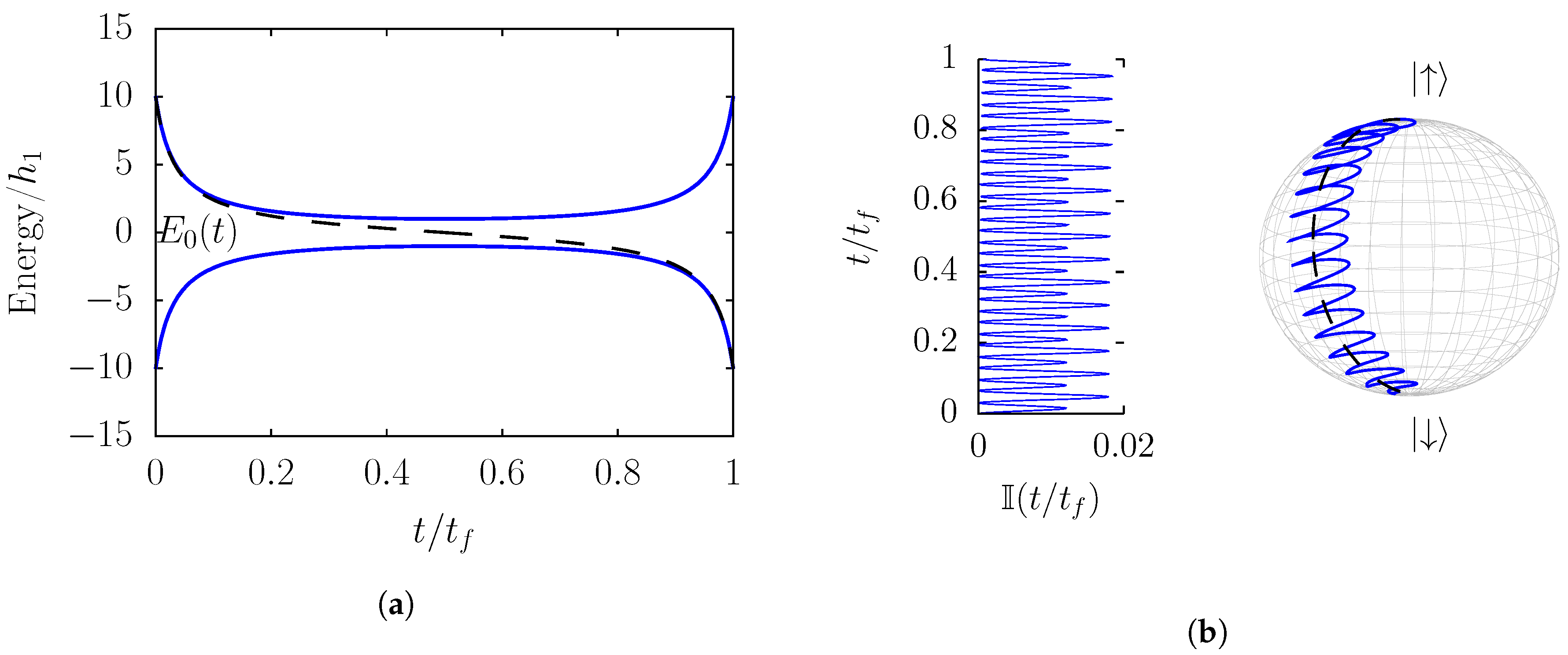
The numerical results discussed in detail in the following are obtained with the values of the dimensionless parameters
. The instantaneous energy levels and the shape of the sweep function of Equation (
28) for these parameters are plotted in
Figure 1a, while the evolution given by the control method, for
is compared with the adiabatic dynamics in
Figure 1b.
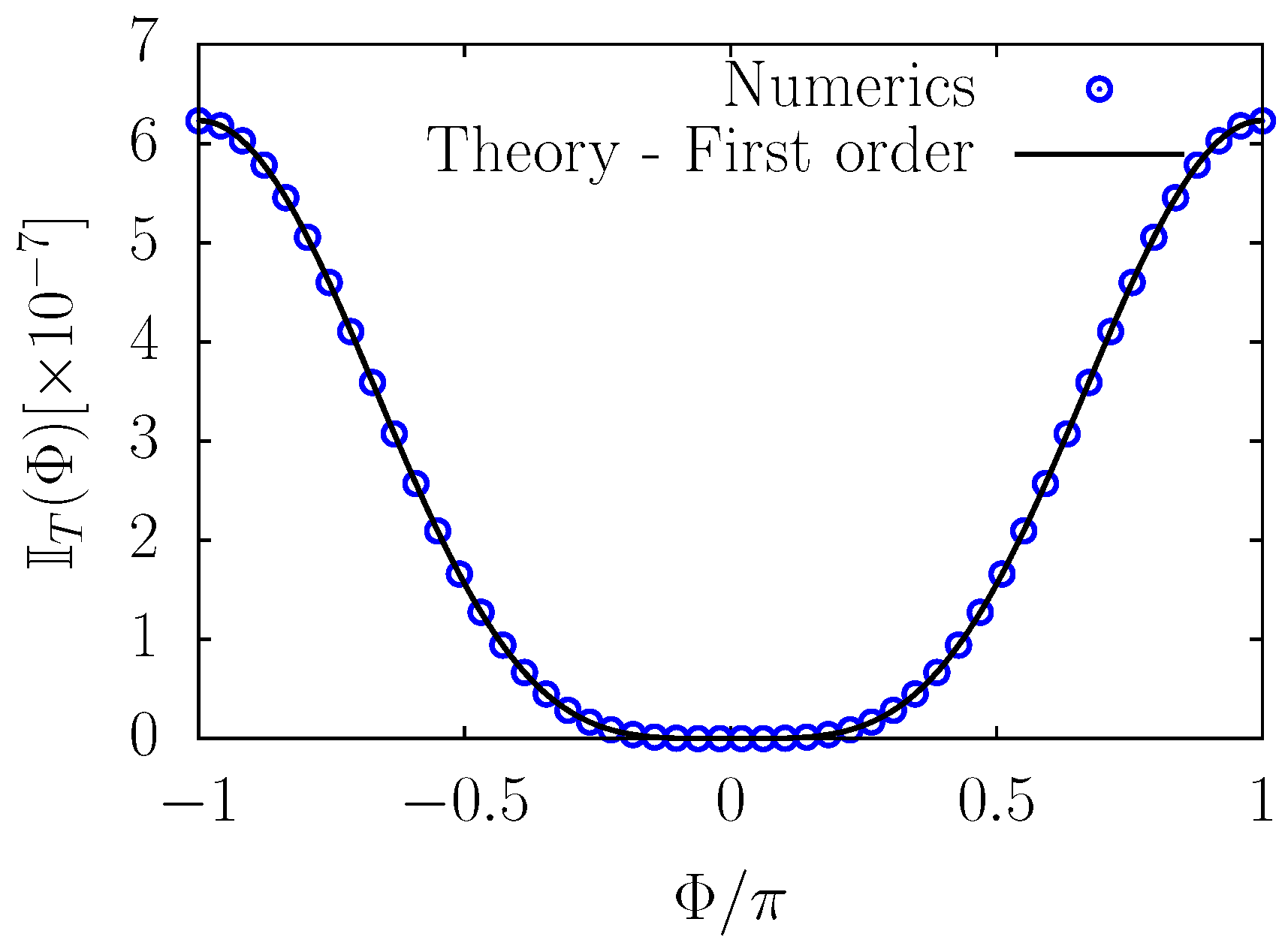
Figure 2 and
Figure 3 show the dependence of the infidelity on the phase offset
for a sweep function of the form of Equation (
28) and for fixed
(so
). Numerical data are indicated with symbols. In
Figure 2, the general behaviour for an ample range of phase errors
is shown. It is appreciable how this is very well described by the oscillating term
of Equation (
26). Nonetheless, such a description becomes ineffective for values of
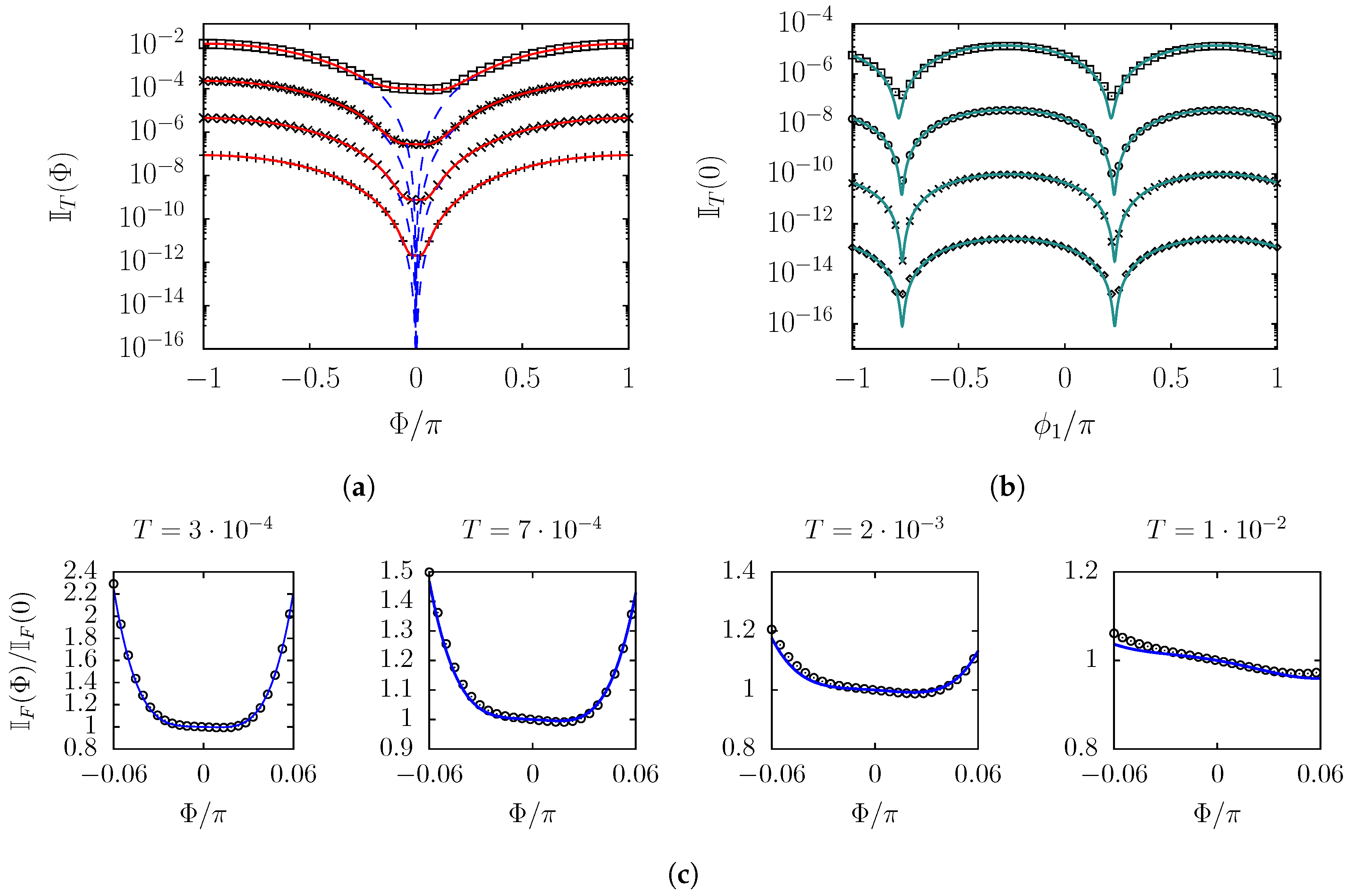
closer to zero. This can be seen from
Figure 3a, where the same general behavior for
is shown for different values of
T, in semilogarithmic scale; the blue dashed line represents the
term in Equation (
26), which is a good description only when
is not small. The behavior near zero is captured by taking into account also the
term (red solid line). The latter introduces an asymmetry around zero with respect to the sign of
which becomes evident for small
: this is shown in
Figure 3c for different values of
T, with the blue line produced by considering both terms in Equation (
26). As
T increases, so does the asymmetry, due to the increasing importance of higher-order terms. From
Figure 3c, it is also interesting to note that the asymmetry can produce a minimum which can be smaller than the value for
, witnessing again the fact that small phase offsets can be beneficial for the control method. Once the relative phase
is fixed, one has still freedom to choose the phase
; although the first term is invariant with respect to this choice, the second one is not. This leaves room for optimization of
for further minimizing the infidelity in each time step. As an example, in
Figure 3b, the infidelity is shown for
and varying
. It is evident that some choices of
can strongly reduce the infidelity with respect to a null
. Numerical simulations show that performing such an optimization in each time step can decrease the infidelity at the end of the whole protocol almost by one order of magnitude.
5. Beyond Two Levels: Two Atoms in a Cavity
In Ref. [
11] an effective counterdiabatic scheme was proposed for speeding up an adiabatic entangling protocol between two superconducting qubits coupled to a transmission line resonator. Due to the complexity of the full multi-level problem, exact analytical expressions in the general case are hardly accessible. Therefore, we discuss the data produced by numerical simulation in the light of the results of the previous section, showing that an insight into the dependence on the phase shift can be obtained also in this scenario. The Hamiltonian of the problem in the rotating wave approximation is of Jaynes–Cummings form:
where
and
—
—are the transition frequencies of the resonator and of the two qubits, respectively, while
denotes the coupling between qubit
k and the resonator. The idea of the entangling protocol is that of exploiting an avoided crossing which emerges between states
and
, where
n is the number of photons while the
denote the states of the qubits, when the two qubits get in resonance with each other far in frequency from
. This avoided crossing results in the dispersive regime
from the emergence of an effective exchange interaction mediated by the exchange of virtual photons through the resonator. If the system starts in the state
, for instance, driving the system adiabatically into qubit resonance produces the entangled singlet state
. In order to bring the two qubits into resonance, one drives their transition frequencies, so that the sweep function is
. For the system starting in
and for
, the correcting Hamiltonian
, derived in Ref. [
11], requires a time-dependent driving of the couplings
g. It reads
where
and
and
are the second and third excited instantaneous eigenvectors of the whole system. As opposed to the two-level case, the nonadiabatic coupling
requires numerical evaluation. This correcting Hamiltonian counteracts unwanted transitions between the two levels involved in the crossing, neglecting effects in the rest of the spectrum, since these are the major obstacle to the desired state transfer.
Let us now suppose that a phase shift is introduced such that, in the above Equation (
32),
.
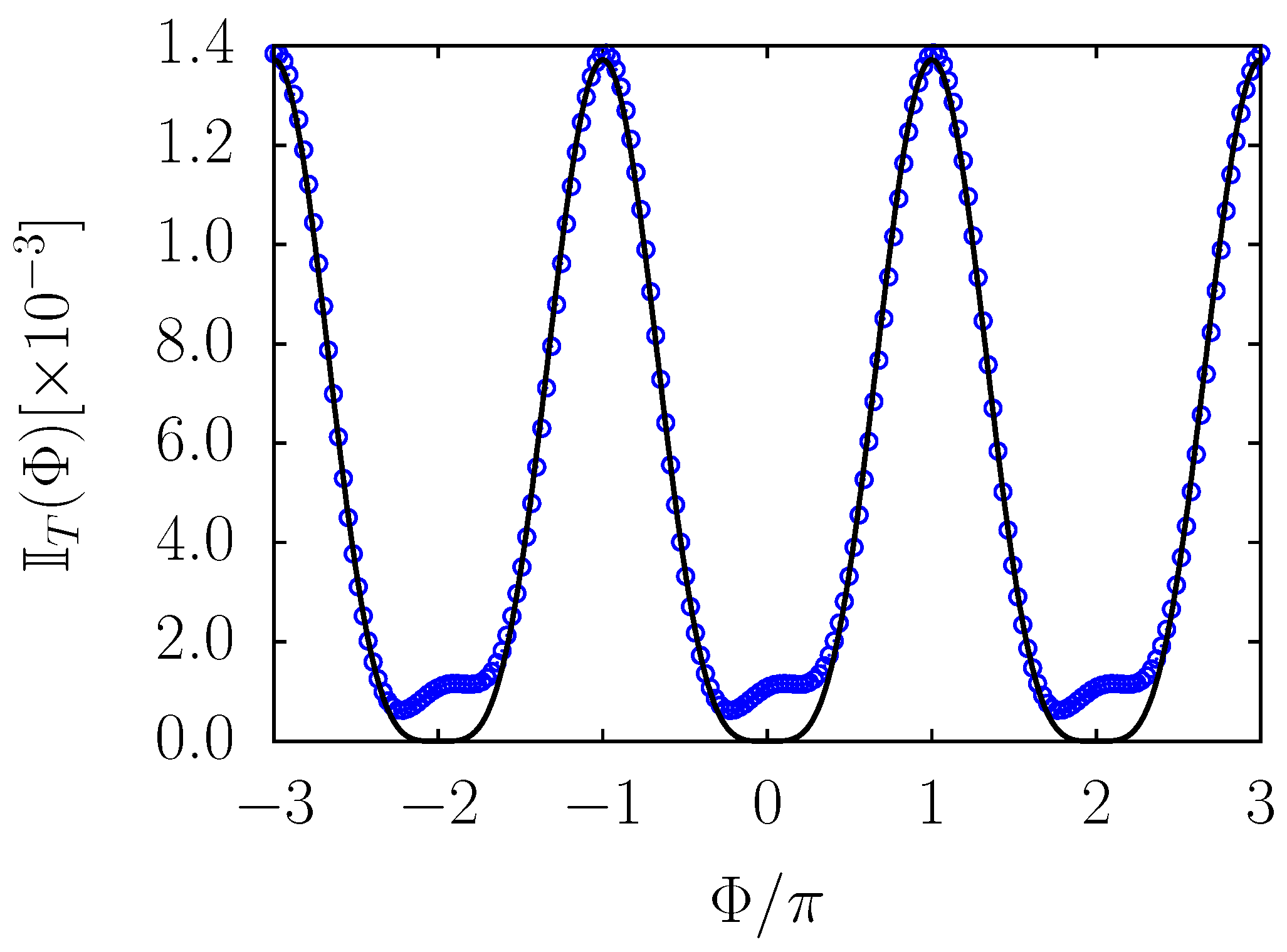
Figure 4 shows the dependence of the infidelity at the end of one time step
T, in units of the unperturbed infidelity
, as a function of the phase error
. The blue symbols are the results of numerical simulations with parameters
GHz,
MHz,
GHz,
MHz and a sweep function of the form
with
and
the minimal width of the anticrossing extrapolated from numerical diagonalization. This is similar to the one in Equation (
28), but it stops (
) at the crossing. One can recognize from
Figure 4 the same general oscillatory behaviour found in
Section 4, which is well captured, far from its nodes, by the black solid line: this line represents a fit with functional dependence as in the first term of Equation (
26), namely
with
k free parameter. In the vicinity of the values
though, higher order effects again come into play. Focusing in the neighborhood of zero, an asymmetry with respect to the sign of
is present, so that for small positive
the infidelity becomes lower than the unperturbed value. We thus see once again that small phase offsets can lead to an accidental improvement of the control protocol. The systematics of this phenomenon further suggest that it can be exploited for optimizing the method.
In conclusion of this analysis, the parameter ranges should be discussed in which these effects are appreciably detectable. This is strictly related to the presence of other secondary phenomena which compete in slightly affecting the value of the infidelity on the same order of magnitude. For the specific framework treated in this section, the essential phenomenon which must be particularly taken into account is that of transitions towards levels other than the two involved in the crossing. We refer to Ref. [
11] for a detailed discussion. The strength of this transition channel depends on the total duration of the protocol and on how good the dispersive-regime approximation is. The latter in turn depends on how large is the ratio
. The effects due to the phase shift are related instead to the strength of second-highest-order term in the expansion of the infidelity in the time step
T, see Equation (
26), which in turn depends on the system parameters and especially on how small
T is. Assuming that
T is sufficiently small for the method to converge at the end of each time step, these effects become visible for larger
T, while they are reduced as
T diminishes as discussed in
Section 4.1. In
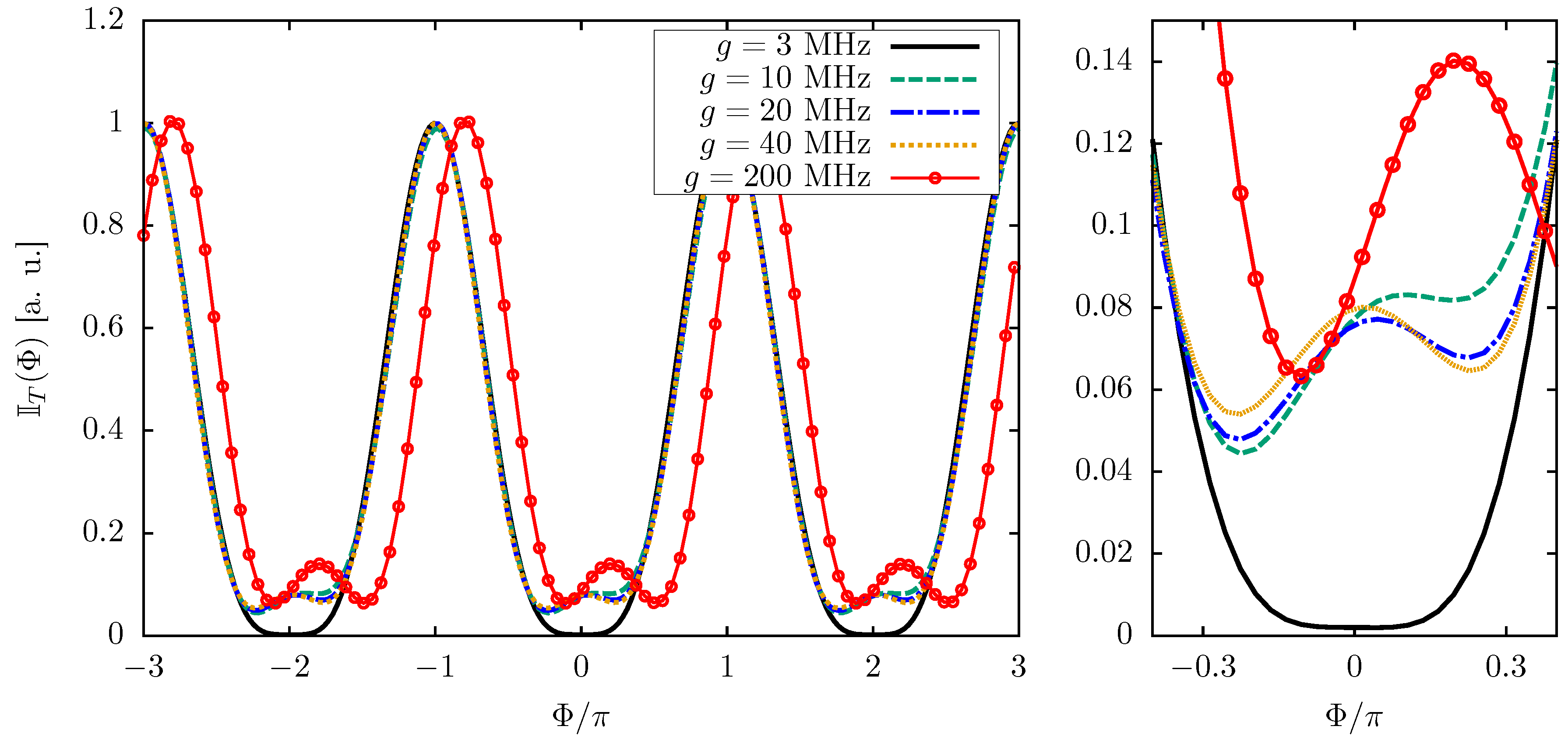
Figure 5 we show how the dependence of the infidelity on the phase offset
behaves as the parameter
g is varied, thus affecting the dispersive-regime approximation. For facilitating the comparison, all the curves are renormalized in such a way that the highest value reached in the interval considered lies at ordinate 1. It is immediately clear the general
oscillating behaviour is robust even if
g becomes large (larger values would challenge the validity of the Hamiltonian (
31) in the experimental platform considered here, due to effects beyond the strong-coupling regime between qubits and resonator [
31]). For small
MHz, transitions to other levels can be neglected and the time step
T is sufficiently small for the
behaviour to be completely dominant. For larger values of
g, asymmetries in the vicinity of zero become more visible. For larger values of
g the whole pattern start to shift with respect to
, indicating the emergence of further effects.


