Abstract
Understanding the spatial pattern of human fishing activity is very important for fisheries resource monitoring and spatial management. The environmental preferences of tropical tuna purse seine fleet in the Western and Central Pacific Ocean (WCPO) were constructed and compared at different spatial scales based on the fishing effort (FE) data from the available automatic identification system (AIS) and commercial fishery data compiled from the Western and Central Pacific Fisheries Commission (WCPFC), using maximum entropy (MaxEnt) methods. The MaxEnt models were fitted with FE and commercial fishery data and remote sensing environmental data. Our results showed that the area under the curve (AUC) value each month based on the commercial fishery data (1°) and FE at 0.25° and 0.5° spatial scales was greater than 0.8. The AUC values each month based on the FE data at a 1° scale ranged from 0.775 to 0.829. The AUC values based on commercial fishing data at the 1° scale were comparable to the model results based on FE data at the 0.5° scale and inferior to the model results based on FE data at the 0.25° scales. Overall, the sea surface temperature (SST), temperature at 100 metres (T100), oxygen concentration at 100 metres (O100) and total primary production (PP) had the greatest influence on the distribution of the purse seine tuna fleet. The oxygen concentration at 200 metres (O200), distance to shore (DSH), dissolved oxygen (Dox), EKE, mixed layer depth (Mld), sea surface salinity (SSS), salinity at 100 metres (S100) and salinity at 200 metres (S200) had moderate influences, and other environmental variables had little influence. The suitable habitat areas varied in response to environmental conditions. The purse seine tuna fleet was mostly present at locations where the SST, T100, O100, O200 and PP were 28–30 °C, 27–29 °C, 150–200 mmol/m3 and 5–10 mg/m−3, respectively. The MaxEnt models enable the integration of AIS data and high-resolution environmental data from satellite remote sensing to describe the spatiotemporal distribution of the tuna purse seine fishery and the influence of environmental variables on the distribution, and can provide forecasts for fishing ground distributions based on future remote sensing environmental data.
1. Introduction
Tuna is important economic species in marine fishery resources and plays an important role in marine ecosystems. Understanding the distribution of tuna fishery resources could help to protect and sustainably utilize tuna fishery resources. Marine environmental factors are important external factors that affect tuna habitat and distribution, and there are many reports on the distribution of tuna and its relationship to environmental variables [1,2,3,4,5]. In previous studies, analyses of fishery conditions in fishing grounds were based on commercial fishing data, and prediction models were established [5]. Log data with high temporal and spatial resolutions are confidential but fraught with uncertainty, especially in the high seas [6], a factor which limits the results of the research. The lack of monitoring and rational management of global marine fishery resources is confounded by the lack of data for small-scale fisheries, and limits fully integrated ecosystem-based fisheries management methods [7].
Recent developments in large data collected from the Automatic Identification System (AIS) now provide dynamic vessel information, allowing the direct observation of over 70,000 industrial fishing vessels. The AIS data have been used for mapping high spatial and temporal resolution fishing effort information and quantifying the overlap between marine species and industrial fishing effort [8,9,10,11,12,13,14,15]. Most of the studies are retrospective and do not capture the underlying dynamic oceanographic processes that result in the spatio-temporal variations. Limited fisheries research on marine environments suggest that the distribution of fishing effort (FE) is driven by environmental factors and can be projected using species distribution models (SDM), together with information on the environment surrounding the fishing observations [7]. This is helpful to understand how the fishing effort may shift in the future and affect fishing communities by running models under different climate scenarios. However, very few studies have evaluated the relationships affecting the monthly spatio-temporal changes of tuna purse seine fishing vessels in the western and central Pacific Ocean (WCPO), which is currently the largest tuna fishing ground in the world and the main operating area of tuna purse seine fishing vessels [16,17]. AIS data allow us to analyse information across a variety of scales. The results based on fishing vessel trajectory information depend on the spatial scale of analysis [18]. The proper scale depends on the specific impact that needs to be investigated.
Understanding the spatial pattern of human fishing activity is very important for fisheries resource monitoring and spatial management. Given the importance of tropical tuna purse seine fishery in the WCPO, we investigate the spatial ecology and drivers of the distribution of the tuna purse seine fishing fleet in the WCPO by developing SDM of fishing distribution from satellite-based AIS data from GFW. SDM have been widely used to explore the distribution of marine species related to environmental factors [19]. Among all the SDM in marine environments, maximum entropy (MaxEnt) has been one of the most popular modelling techniques since its appearance in 2006, and it has shown robust predictive accuracy [19]. We constructed environmental niche models at different spatial scales, using a MaxEnt modelling approach that relates the location of fishing events to different environmental conditions and compares them to a set of pseudoabsence points (areas of no observed fishing). By comparing the conditions where fishing was observed to locations where fishing was not observed, we could decipher which environmental conditions seem to be preferred by tuna purse seine in the WCPO at different spatial scales and to find the proper scale based on the goodness of models. A comparison of the results between commercial fishery data and FE was used to determine whether the EF data could be used to understand the species environment habitat. The analysis could provide scientific support for the use of these data by countries and Regional Fisheries Management Organisations in fishery resource management.
2. Materials and Methods
2.1. FE Data, Study Area and Commercial Fishery Data
The Global Fishing Watch (GFW) organization provides the fishing operation times of 16 different types of fishing vessels worldwide in each grid every day from 2012 to 2020 (https://globalfishingwatch.org/, accessed on 6 January 2022). The data include date, latitude, longitude, Maritime Mobile Service Identities (MMSIs), sailing time and fishing time information. The spatial resolution is 0.1 degree, and the temporal resolution is in days. The GFW fishing effort (FE) data of classified purse seine tuna fishing vessels were considered in this paper.
The GFW first processes the raw AIS data through a series of algorithms designed to filter out corrupt or incomplete records and assigns additional information to each AIS datum, such as the distance from shore, depth, and time since the vessel’s previous AIS position. The data are then ready for the fishing detection model. A convolutional neural network (CNN) model was constructed by Kroodsma et al. [11] to distinguish all fishing positions from non-fishing positions for every AIS position, excluding squid jigger vessels. This algorithm identifies fishing events with > 90% accuracy. The time associated with the fishing positions is considered the apparent fishing activity. The fishing effort in each area every day is calculated by summarizing the fishing hours for all fishing vessels in that area. This method and its data have been applied to many research fields (https://globalfishingwatch.org/publications/, accessed on 6 January 2022). The details of the CNN model are described in the supplementary materials of Kroodsma et al. [11].
The time series of the vessel numbers and FE for the purse seine tuna fishery in the WCPO from 2012 to 2020 is shown in Figure S1. The vessel number and FE for the purse seine tuna fishery in the WCPO during 2012 to 2020 showed two distinct stages; i.e., the accumulated FE and vessel number sharply increased from 2012 and 2015 for more and more large vessels (>24 m) equipped with AIS devices, and then there was oscillation during 2015 to 2020. We used the data starting from 2015 for analysis. The traditional tuna purse seine fishing area was mainly distributed in the area of the WCPO spanning from 130°–150° W to 20° S–20° N. Figure 1 shows the spatial maps of the fishing locations from 2015 to 2020 in this area. The tuna purse seine fishing positions were mainly distributed near the equator in the area of 20° S–20° N. In order to spatially constrain the pseudo-absences to waters near the presences, we defined this region (130°–210° E; 20°S–20° N) as the study area. In the study area, the tuna purse seine fleet mainly fished in the Exclusive Economic Zones (EEZ). There are several EEZs (Howland, Baker, and Jarvis Islands) and Marine Protected Areas (MPAs, Phoenix Islands and Pacific Remote Islands) where fishing is prohibited (Figure S2). To avoid confounding the model, the above areas were masked from the study area. The MPA data were downloaded from https://mpatlas.org/zones/ (accessed on 22 January 2022), and the EEZ data were downloaded from https://www.marineregions.org/downloads.php (accessed on 22 January 2022).
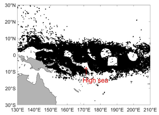
Figure 1.
The spatial distribution of fishing locations during 2015–2020 (The red arrow points to an empty area).
Commercial tuna purse seine fishery data in the WCPO were compiled from the Western and Central Pacific Fisheries Commission (WCPFC) (Figure S3). The data included longitude, latitude, catches, and net times. The time resolution was one month, and the spatial resolution was 1° × 1°.
2.2. Environmental Data
In previous studies, temperature, salinity, SSH, chlorophyll-a (Chla), dissolved oxygen and primary production were identified as playing important roles in the spatial distribution of tuna [3,4,5,20,21,22,23]. The daytime swimming depth of tuna detected with FADs showed that tuna occasionally dive to approximately 100 m or deeper in the Pacific, while most of the catch by tuna purse seines is usually from shallower (<100 m) waters (Matsumoto et al., 2016). The spatial and vertical distribution of tuna relates to subsurface environmental factors and may also have an impact on the distribution of tuna and surface fishing vessel operations. In addition, there is a need to incorporate a third dimension relating to the vertical positions of tuna into the models to improve the precision and utility of the models [24,25]. Therefore, environmental variables such as water temperature, salinity, dissolved oxygen, chlorophyll, and primary productivity at the surface and at depths of approximately 100 m and 200 m were selected as input variables for the model in this study. All the surface and subsurface environmental data were downloaded from the Copernicus Marine Environment Monitoring Service (CMEMS) website https://resources.marine.copernicus.eu/?option=com_csw&task=results (accessed on 20 January 2022). The temperature, salinity, sea surface height, mixed layer depth, geostrophic zonal velocity (U) and geostrophic meridional velocity (V) came from “global-analysis-forecast-phy-001-024-monthly” product. The Dissolved Oxygen, total Chlorophyll and total Primary Production came from “global-reanalysis-bio-001-029-monthly” product. All the environmental factors used in this work were described in Table S1. It should be noted that the depth of dissolved oxygen, chlorophyll, and primary productivity collection was not at exactly 200 metres, but at an approximate depth. The time resolution was a monthly average. The time coverage was from January 2015 to December 2020. Sea surface temperature front (SSTf), thermocline, and Eddy kinetic energy (EKE) also affect tuna distribution and fishing vessel operations [22,26]. These three variables were calculated based on the downloaded remote sensing environmental data. The ocean front detection algorithm based on chlorophyll and sea surface temperature satellite images proposed by Belkin and O’Reilly [27] was applied to compute the SSTf. Thermocline depth was calculated based on the variable representative isotherm method, as recommended by Fiedler [28]:
where T(mld) is the temperature at the depth of the mixed layer, tem is the temperature at the sea surface, and tem400 is the temperature at a depth of 400 metres.
2.3. Geographic and Topographic Variables
Studies have shown that fishing operations are related to the distance to shore (DSH) and distance to port (DPT), as well as bathymetry (depth) [7]. In this paper, these three statistical variables were selected as model input variables. The above statistical variables were downloaded from https://globalfishingwatch.org/data-download/ (accessed on 6 January 2022).
2.4. Data Processing
FE is detected and calculated, as hours of fishing, for individual fishing gear. We filtered the GFW FE estimates spatially to select only tuna purse seine events in the WPCO. The FE data were those constrained only to locations that had > 0 fishing hours. We focused on the monthly environmental variability of the distribution of the fishing effort. The raw daily FE information available at a resolution of 0.1° degrees was converted into a monthly average, and 12 monthly environmental niche models were constructed based on each month’s environmental data. Presence was defined as positions where the FE > 0. Pseudoabsence points were randomly sampled from the background by the models. Three different spatial scales (0.25° × 0.25°, 0.5° × 0.5° and 1° × 1°) were used to compare spatial scale effects. The data from 2015 to 2019 were used as the training dataset, and the data from 2020 were used to test the prediction ability of the model’s data. The spatial and temporal resolutions of the input variable data were processed to match the FE data.
If a high correlation exists among environmental variables, their percent contributions should be interpreted with caution. If environmental variables are correlated, their marginal response curves can be misleading [29]. The variance inflation factor (VIF) and kappa coefficient were calculated to evaluate the multicollinearity of the environmental variables. The larger the VIF and kappa coefficient are, the greater the possibility of collinearity between the independent variables. If the VIF exceeds 10 or the kappa coefficient is greater than 100, the regression model has multicollinearity. In this study, a regression model was established between the 22 environmental factors and the FE, and the VIF score and kappa coefficient were calculated. We eliminated multicollinearity by deleting related variables to reduce the VIF and kappa coefficient values.
2.5. MaxEnt Model Construction
MaxEnt software version 3.4.4 was used to perform the analyses in this paper. The environment layer comprised the monthly average of each month from 2015 to 2019 converted into an ESRI ASCII grid format. Twelve models were established, one for each month, to examine seasonal changes. The monthly average environmental layer of each month in 2020 was used as the projection layer to calculate the habitat suitability index (HSI) value in 2020. All the models were constructed based on the default setting for the regularization parameter. The number of background points (BPs) was 10,000 for the 0.5° × 0.5° and 1° × 1° spatial resolutions, and 100,000 for the 0.25° × 0.25° spatial resolution. The maximum number of iterations was 500, and automatic features were selected. A regularization multiplier was also introduced, to reduce overfitting. The background points were selected from the geographical space by default and treated as pseudoabsences. A response curve was established, and a jack-knife test was used to obtain alternate assessments of which variables were the most important in the model, and a response curve was used to plot the distribution map of the probability of occurrence of purse seine fishing operations in the function of the environmental variables. The presence data were randomly split into 75% training and 25% validation points for each month of the models. The training dataset was used to fit the models, and the validation dataset was used to validate the performance of the models.
2.6. Model Selection and Validation
The area under the curve (AUC) of the receiver operating characteristic (ROC) curve of the validation dataset was used to evaluate the goodness of fit of the MaxEnt models [30]. The AUC value ranged from 0 to 1. The performance of the model was demonstrated by the high value of the AUC, in which a value greater than 0.7 was considered to be indicative of a useful model [30]. The validation of the best-fitting monthly models was applied to calculate the HSIs during 2015–2019 and 2020. The spatial maps were plotted by overlaying the actual fishing operation locations to deduce their prediction ability.
3. Results
3.1. Multicollinearity
A regression model was established between the 22 environmental factors and the FE to calculate the VIF values of each variable and the kappa coefficient value. The original kappa coefficient was 459, and the maximum VIF was 39.91, derived from the thermocline (Table S2), which suggested a high multicollinearity among the 22 independent variables. The correlations between the thermocline and SST, Chl and PP, and T200 and S200 were high, as their correlation coefficient values were greater than 0.9. The thermocline, Chl and T200 were deleted due to their VIF values. Then, all the remaining VIF values were smaller than 5.4, and the kappa coefficient was smaller than 50.
3.2. Modelling Performance
The AUC values for all months based on the WCPFC and FE data at the spatial scales of 0.25° and 0.5°were greater than 0.8 (Table 1), which suggested that the performance of all the models was very good. The AUC value of the model constructed based on fishing effort data at a 1° spatial resolution was still above 0.7. These models are still considered to have high predictive power, although there were models with higher resolution. The AUC values based on the EF data were greater as the spatial resolution increased. The results derived from fishery data were similar to the FE data at 1°and 0.5° scales, and inferior at 0.25° spatial scales.

Table 1.
Summary statistics derived from different models.
3.3. Relative Importance of Environmental Factors
The average importance of each variable calculated based on the training data set for each model is shown in Table 2 and Figure S4. The contribution of each factor in each month of the four models is listed in Tables S3–S6. The jack-knife test results of the variable importance derived for each model are shown in Figures S5–S8. The contribution of each factor in each month differed for each model (Tables S3–S6). The SST, T100, PP and O100 always had high average scores in the four models, except those based on 1° EF data, which contributed significantly to the training of the model (Table 2 and Figure S4). The average contribution rates of the O200, DSH, EKE, Mld, Dox, SSS, S100 and S200 exceeded 1%, indicating that these variables had a moderate impact on the distribution of purse seine tuna fleet, while other variables had little effect. The green bars of the important variables above in the jack-knife graph did not exceed the red bar each month, indicating that all the useful information was not already contained in the other variables (Figures S5–S8).
Table 2.
The average contributions of the environmental variables to the Maxent model.
3.4. Purse Seine Tuna Distribution in Relation to Important Environmental Variables
The response curves for the important variables each month, resulting from the four models, are shown in Figures S9–S12. Overall, the probability of the occurrence of tuna purse seine vessels increased as SST exceeded 28 degrees C; however, when SST was lower than 26 °C, the probability of occurrence tended towards zero probability (Figure S9). The response of tuna purse seine fleets to T100 was similar to that of the SST. The purse seine tuna fleet did not appear in areas where the T100 was below 24 °C in most months, and were more likely to appear in areas where the T100 was greater than 26 °C (Figure S9).
There was a difference in the influence curve of the O100 on the probability of the occurrence of the purse seine tuna fleet each month when the spatial scale was lower than 0.5°. Meanwhile, the distribution showed consistency when the spatial scale was 0.25°. The probability was higher in areas where the O100 was less than 250 m mol/m3 in each month when the spatial scale was 0.25°. In some months, purse seine tuna fleets were more likely to occur in the 200–250 mmol/m3 area when the spatial scale was lower than 0.5°.
The influence curve of the PP based on the FE data was different than that based on the commercial fishery data. The probability of occurrence of the purse seine tuna fleet presented a logarithmic function distribution. From 0 to 5 mg·m−3·day−1, the probability of occurrence of the purse seine tuna fleet increased sharply based on both the FE and commercial fishery data. However, the probability decreased after 5 mg·m−3·day−1.
The occurrence locations of the purse seine tuna fleet were mostly located in areas where the SST and T100 were greater than 28 °C and 25 °C, respectively. The subsurface dissolved oxygen was relatively low near the equator in the WCPO. Conversely, the PP was higher near the equator. Purse seine tuna fleets were mainly located in this area (Figure 2). The frequency distributions based on the FE data and commercial fishery data were similar (Figures S13–S16). The frequency results showed that the preferred purse seine tuna fleet ranges for SST, T100, O100 and PP were 28–31 °C (98.34%), 26–30 °C (94.5%), 190–250 mmol/m−3 (78.06%) and 0–10 mg·m−3·day−1 (92.45%), respectively, based on FE data at a 0.25 spatial scale (Figure S13).
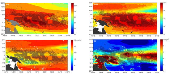
Figure 2.
The spatial distribution of high FE (greater than the mean value) locations overlayed with important factors at the 0.25 spatial scale during 2015 to 2019.
3.5. Prediction of Habitat Suitability
The monthly HSI map of 2015–2019 and the predicted map of 2020 are shown in Figures S17–S24. The monthly HSI spatial distributions of 2015–2019 based on FE data and commercial fishery data were similar. The monthly HSI map of 2015–2019 was mainly distributed near the equator and had little seasonal change. The high-value habitat area in the Southern Hemisphere shrank towards the equator in terms of latitude and extended westward from January to July. The high value area in the Southern Hemisphere habitat reached the equator, and its zonal coverage area was the narrowest in July. Subsequently, the high-value areas of the Southern Hemisphere habitats extended south and west until December, when the zonal coverage of the high-value areas reached the widest value of the year. The purse seine tuna fleet mainly appeared in areas with a habitat index greater than 0.6 from 2015 to 2019.
The spatial distribution of the suitability index predicted by the model based on FE data was different from that of the model based on commercial fishery data, and both showed an obvious variation in 2020. The spatial distributions of the predicted HSIs were similar at the 0.25 and 0.5° spatial scales based on FE data; the high value area gradually extended westward from January to June, and the absolute value of the habitat suitability index gradually increased. The lowest habitat suitability index value was found in July. The absolute value and coverage area of the habitat suitability index from August to December gradually increased again. There was no obvious pattern of predicted HSI at the 1° spatial scale, based on either FE data or commercial fishery data. However, the high value coverage area based on FE was greater than that based on commercial fishery data each month. The purse seine tuna fleets were mainly located in the high value area of the habitat suitability index each month at the 0.25° spatial scales, but that was not always the case in the model based on commercial fishery data.
4. Discussion
4.1. MaxEnt Model Construction
The traditional purse seine fishing area was considered the study area in this paper. The location of tuna purse seine fishing was concentrated at 15° S-–15° N. In addition to this zonal area, there were scattered fishing points. There were 1516 pixels (excluding land, EEZs and MPAs) in the region (130°–210° E; 15° S–15° N). There were an average of 846 FE positions in this area. Considering the selection of background points (pseudoabsence points) at a 1° spatial scale, the latitude range of this paper was 20° S–20° N. There were EEZs and MPAs in this area, and most of the fishing points were in the EEZs. To negate the bias effect of the MPAs and EEZs as background points (BPs), the EEZs and MPAs in which fishing was prohibited were masked in this paper. However, the results from the models with these zones masked showed that there was little difference between models with masked data and those without masked data (Tables S7 and S8). The MaxEnt model did not select sample data from the EEZs and MPAs location when they was included in study area when there was no fishing activity. The similar sample data location suggests that the EEZs and MPAs did not bring model bias.
Some researchers [31] suggest that the default number of BPs is insufficient for a representative analysis of the variability of natural factors over a wide area. If the BP sample includes all the landscape possibilities, it would be sufficient for analysing the distribution properties of natural factors. Therefore, different BPs were set at different scales in this paper. There were 44,094, 11,235 and 2946 pixels (excluding land, EEZs and MPAs) at 0.25°, 0.5° and 1° spatial scales, respectively. At minimum, more than 40% of cells used in the analysis can represent all of the variety of combinations of natural factors in the study area. The number of BPs set in this paper were sufficient. Twelve models were established which could limit the amount of data that go into each model, especially if the fishing effort had high temporal intra-annual variability. However, the FE data in each month at each spatial scale were sufficient to cover the fishing grounds and had low temporal intra-annual variability (Figures S17–S24).
A correction layer was not applied in constructed models, but the output of models show that the locations of the training and testing data sets selected by the software were all near to the presences data (Figures S25–S28). The figures suggest that the background points were not randomly selected from the geographical space by the software, since the sample data and presence data had similar bias, so then sampling bias is negligible for this choice of background.
This study described the distribution of the purse seine tuna fleet as characterised by a set of environmental and statistical variables. Some of these variables (e.g., sea surface temperature, sea surface height, geostrophic currents, salinity, and chlorophyll-a) have been used in previous tuna habitat and distribution studies, but descriptions of habitat preferences based on other variables (e.g., MLD, PP, Dox, DSH, and DPT) are rarely found in the literature. The results showed that Dox and PP were two important variables, and a third dimension relating to the vertical positions of tuna also needs to be incorporated in the models.
Fisheries data have been criticized for being biased because the CPUE may not accurately reflect the population abundance due to changes in fishing practices, the efficiency of the fleet or environmental effects on catchability, among other factors [32,33]. For example, a fishery population may actually exist even where there is no catch, due to failures of the tuna purse seine vessel operations. The fishing intensity information is also related to the fishing efficiency and power of the fishing fleet. The FE information indicates the presence locations of the tuna population, regardless of the success or failure of the fishing vessels. The tuna occurrence records derived from the FE and commercial fishery data were used to fit the MaxEnt models in this paper.
MaxEnt models are promising tools that have been verified prior to other species distribution models [34]. Melo-Merino et al. [25] counted published papers on marine ENMs and SDEs from 1990 to 2016 and stated that the MaxEnt was the most frequently used method, far exceeding other machine learning and statistical models, and has been proven to be superior to other niche models. We used MaxEnt models to relate the fishing locations in the WCPO to environmental conditions and evaluated the model performance.
The AUCs were higher than 0.8 for the models in all months (except at the 1° spatial scale) based on the FE data, which suggested that the models were in good agreement with the testing data. Predicted potential habitat suitability maps at high spatial resolutions also showed better spatial matches with actual fishing positions. However, three environmental variables (sea surface chlorophyll, temperature at 200 metres and thermocline) were excluded from the MaxEnt model due to collinearity issues. It should be noted that these three environmental variables had important effects on the purse seine tuna fishery distribution in previous studies [34]. The effects of these three environmental variables were represented by other factors included in the MaxEnt model.
4.2. Spatial Scale Effects
Spatial scale has always been an important factor in ecological research. The AUC values were greater as the spatial resolution increased based on the EF data. The AUC values based on the FE data showed that the results at the 0.5° spatial scale were comparable to those of the model constructed based on commercial fishery data.
Except for the model constructed based on the FE data at a 1° spatial precision, the AUC values of all the other models in all months were higher than 0.8, indicating that the models were in good agreement with the testing data. The AUC values showed that the model results based on fishing effort data under spatial accuracies of 0.25° were better than other models. Fishing effort data with a spatial accuracy higher than 0.5° can be used to analyse the relationship between the tuna fishery and the environment in the WCPO.
The response curves for the important environmental variables between different spatial scales presented little change. This suggest that the fisheries have similar responses to the environment at different spatial scales. This may be due to the study area covering the entire WCPO. Previous studies have showed that the environmental preference changes at different spatial investigated scales [7,11,12]. The spatial overlay map showed a blank area near the coastline of Papua Guinea Island due to the coarse spatial resolution, but there were fish catch data located in this area. The HSI map resulting from the high spatial resolution data showed that the HSI values were high in this area. This suggests that commercial fishery data at the 1° spatial scale are not suitable for small-scale spatial analysis. High-resolution fishing effort data were a suitable substitute in fine scale fishery resource management. The prediction overlay map based on the commercial fishery data showed that there were many fishing positions located in low HSI areas from January to May. In contrast, the fishing positions were more consistent with the high HSI based on high-resolution FE data. This may be due to the potential relationship information being captured by the model with high spatial FE data, while it was smoothed with low spatial commercial data. This suggest that the results based on high-resolution FE data are more reliable in fisheries planning.
4.3. The Contribution of Environmental Factors
The predicted HSI maps show seasonal variation based on FE, and commercial fishery data showed seasonal variation, which mainly is caused by ocean environmental changes each month, especially in the most important environmental variables. The results showed that the SST, T100, O100 and PP were the most important environmental variables impacting the purse seine tuna fleet. The purse seine tuna vessels primarily target small skipjack (Katsuwonus pelamis), yellowfin tuna (Thunnus albacares) and bigeye tuna (T. obesus). The four important variables above reflect the physiological and ecological habits of these targeted tuna [35] and influence the distribution of the purse seine tuna fleet. The species above can swim fast and deep, and usually display distinctive daily depth distributions and vertical movement patterns [36,37,38,39]. The daytime swimming depth of tuna has been detected with FADs and shows that tuna occasionally dive to approximately 100 m or deeper, while catches by a tuna purse seine fleet are usually in shallower (<100 m) waters [40]. Although tuna have a unique physiological feature that allows them to tolerate low ambient temperature and oxygen levels for a short period of time [41], both sea temperature and dissolved oxygen have a strong impact on the biological processes of tunas and determine their spatial distribution [42,43]. This is especially true for small tuna that have a lower sea temperature and dissolved oxygen tolerance. Therefore, the subsurface water temperature and dissolved oxygen have important effects on purse seine tuna fleet.
The swimming depth and spatial distribution of tuna are regulated by temperature and dissolved oxygen [42,43]. If their potential vertical habitat is compressed in the upper layer, pelagic fish populations will have an increased vulnerability to purse seine tuna vessels [44]. The spatial distribution of the tuna eventually influences the surface gear distribution [45]. Dear et al. [43] characterized the potential vertical habitat of four important tuna species using comfort values for temperature and dissolved oxygen, and found that tuna were restricted to depths below 100 m between 5° S and 10° N, and noted that a low dissolved oxygen level was a more important factor than water temperature in restricting the vertical movement of tuna. Changes in the water structure associated with climate change may also influence their vertical distribution [42,45], and eventually impact their catchability by surface gear.
However, dissolved oxygen is rarely used to describe tuna habitat and distribution habitat preferences compared with water temperature. Another variable, PP, was also rarely examined in previous studies but showed an important effect in the MaxEnt model. Prey is also an important factor that affects the spatial and vertical distribution of tuna [41]. The distinct swimming depth distribution of the tuna was driven by the vertical migrations of their prey. The tuna characteristically descended to deep depths to prey on small nektonic organisms (squid, euphausiids, and mesopelagic fish) of the DSL (deep scattering layer) or SSL (sound scattering layer) after dawn [41]. Bigeye tuna forage in the DSL, while skipjack and yellowfin tuna forage in the SSL [42]. Yen and Lu [21] have shown that higher primary productivity also attracts tuna. Kroodsma et al. [11] also concluded that primary productivity has an impact on the distribution of global fishing vessels. Primary productivity supports the ecosystem and has an important influence on the food sources, spawning habitats, survival rates, recruitment, and biomass of tuna [21]. Primary productivity provides nutrients for zooplankton that attract tuna prey such as herrings, anchovies, and sardines.
4.4. Distribution of Vessel Operations in Relation to Environmental Variables
The spatial distributions of traditional fishing grounds are essentially concentrated in the WCPO, in the westward domain of the dateline and close to the warm-pool area (Figure S3). Skipjack tuna was the dominant target species of the purse seine fishery, followed by yellowfin tuna [46]. Skipjack tuna follow a brief route to the south for spawning and retreat to the north during the summer. FE extended south to the Solomon Islands in quarters one and four, and they withdrew from the south in quarters two and three in both datasets [21].
The average annual contribution rate of four important variables accounts for more than 70% of the findings, which suggests that the distribution of purse seine tuna fleet in the WCPO is mainly related to the four important variables. The operation locations of purse seine tuna vessels were near the equator in the western and central Pacific Ocean, which corresponds with the log data [47]. Tuna are likely to appear in areas where the SST and water temperature at 100 m exceed 28 °C and 26 °C, respectively, which is consistent with the results of [48]. We did not consider the impact of climate change in this paper, but the results also suggested a clear geographic and water temperature overlap between the preferred habitat of the main tuna species [40] and a suitable fishing habitat for pelagic purse seine fleets in the WCPO. This supports the reasonable use of the fishing vessel trajectory.
The purse seine tuna fleet did not appear in areas with maximum dissolved oxygen, which may be related to the water temperature and PP. In areas with maximum dissolved oxygen, the water temperature and PP were relatively low. Meanwhile, the purse seine tuna fleet did not occur in the area where the dissolved oxygen was too low (Figure 2). A lower dissolved oxygen may drive the target species to swim to a moderate dissolved oxygen area where the temperature and PP are suitable. Primary productivity provides nutrients for phytoplankton, has indirect relationships with the foraging distribution, and affects the predators. The productive area may correspond to oceanic fronts in the region, represented by ambient phytoplankton. Areas with large PP values are more attractive to prey, which means that tuna prefer to aggregate there and draw vessel fishing to these areas.
5. Conclusions
In this study, MaxEnt models were constructed to evaluate the influence of environmental factors on tuna purse seine fishing activity. The results showed that the FE data with a spatial resolution higher than 0.25° are suitable to analyse the relationship between the purse seine tuna fishery and the environment in the WCPO, and can provide forecasts for fishing ground distributions based on future remote sensing environmental data. The SST, T100, O100 and PP were the most important environmental variables impacting the purse seine tuna fleet. The average annual contribution rate of four important variables was more than 70%. The probability of occurrence of tuna purse seine vessels increased as SST and T100 became higher. The probability was higher in areas where the O100 was less than 250 m mol/m3, and then sharply decreased. Conversely, a logarithmic function distribution was presented which relates to PP. The frequency results showed that the preferred purse seine tuna fleet ranges for SST, T100, O100 and PP were 28–31 °C (98.34%), 26–30 °C (94.5%), 190–250 mmol/m–3 (78.06%) and 0–10 mg·m–3·day–1 (92.45%), respectively, based on FE data at a 0.25 spatial scale.
Supplementary Materials
The following supporting information can be downloaded at: https://www.mdpi.com/article/10.3390/fishes8020078/s1, Figure S1: The fishing effort and number of fishing vessels during 2012-2020;Figure S2: The spatial distribution of MPA and EEZ locations; Figure S3: The spatial distribution of commercial fishery data during 2015-2020;Figure S4: The average importance scores for different MaxEnt models; Figure S5: Jackknife test results of the variable importance derived for each month in the GFW_0.25° model. The blue and green bars correspond to the effect on model gained by using and sequentially removing each variable from the model, respectively; Figure S6: Jackknife test results of the variable importance derived for each month in the GFW_0.5° model. The blue and green bars correspond to the effect on model gained by using and sequentially removing each variable from the model, respectively; Figure S7: Jackknife test results of the variable importance derived for each month in the GFW_1° model. The blue and green bars correspond to the effect on model gained by using and sequentially removing each variable from the model, respectively; Figure S8: Jacknife test results of variable importance derived for each month in the WPFCF model. The blue and green bars correspond to the effect on model gained by using and sequentially removing each variable from the model, respectively; Figure S9: Response curves for important variables in all months in the GFW_0.25° model; Figure S10: Response curves for important variables in all months in the GFW_0.5° model; Figure S11: Response curves for important variables in all months in the GFW_1° model; Figure S12: Response curves for important variables in all month in the WPCFC model; Figure S13: Frequency distribution of important variables based on EF data at the 0.25° spatial scale; Figure S14: Frequency distribution of important variables based on EF data at the 0.5° spatial scale; Figure S15: Frequency distribution of important variables based on EF data at the 1° spatial scale; Figure S16: Frequency distribution of important variables based on commercial fishery data at the 1° spatial scale; Figure S17:The spatial distribution of fishing locations (black dots) overlain on habitat suitability maps for each month during 2015-2019 in the GFW_0.25° model; Figure S18: The spatial distribution of fishing locations (black dots) overlain on habitat suitability maps for each month in 2020 in the GFW_0.25° model; Figure S19:The spatial distribution of fishing locations (black dots) overlain on habitat suitability maps for each month during 2015-2019 in the GFW_0.5° model; Figure S20:The spatial distribution of fishing locations (black dots) overlain on habitat suitability maps for each month in 2020 in the GFW_0.5° model; Figure S21:The spatial distribution of fishing locations (black dots) overlain on habitat suitability maps for each month during 2015-2019 in the GFW_1° model; Figure S22: The spatial distribution of fishing data locations (black dots) overlain on habitat suitability maps for each month in 2020 in the GFW_1° model; Figure S23: The spatial distribution of fishery data locations (black dots) overlain on habitat suitability maps for each month during 2015–2019 based on fishery data; Figure S24: The spatial distribution of fishery locations (black dots) overlain on habitat suitability maps for each month in 2020 based on fishery data; Figure S25: The spatial distribution of sample data in the GFW_0.25° model based on FE data. Red dots show the presence locations used for training, while violet dots show test locations; Figure S26:The spatial distribution of sample data in the GFW_0.5° model based on FE data. Red dots show the presence locations used for training, while violet dots show test locations; Figure S27: The spatial distribution of sample data in the GFW_1° model based on FE data. Red dots show the presence locations used for training, while violet dots show test locations; Figure S28: The spatial distribution of sample data in the GFW_1° model based on fishery data. Red dots show the presence locations used for training, while violet dots show test locations; Table S1: Summary of environmental data and description; Table S2: Summary of VIF statistics; Table S3: Contribution of each factor in each month for the GFW_0.25° model; Table S4: Contribution of each factor in each month for the GFW_0.5° model; Table S5: Contribution of each factor in each month for the GFW_1° model; Table S6: Contribution of each factor in each month for the WPCFC model; Table S7: Summary statistics derived from different models without mask; Table S8: The relative average contributions of the variables to the Maxent model without masks.
Author Contributions
All authors contributed to this study. Conceptualization, S.Y., S.Z. and W.F.; methodology, S.Y., S.Z., T.C. and L.Y.; software, S.Y. and L.Y.; validation, S.Y., F.W., T.C. and Y.F.; investigation, S.Y. and L.Y.; resources, W.F.; data curation, S.Y., L.Y. and Y.F.; writing—review and editing, S.Y. and W.F.; supervision, S.Y., S.Z. and W.F. All authors have read and agreed to the published version of the manuscript.
Funding
This research was funded by the National Key R&D Program of China (2019YFD0901405, 2019YFD0901404), the Special Funds of Basic Research of the Central Public Welfare Institute (2019T09), and the Shanghai Science and Technology Innovation Action Plan (19DZ1207504).
Institutional Review Board Statement
Not applicable.
Data Availability Statement
Publicly available datasets of vessels number were analysed in this study. These data can be found here: https://globalfishingwatch.org/, accessed on 6 January 2022.
Acknowledgments
The authors are grateful to the Global Fishing Watch for the GFW website. We acknowledge the use of oceanic parameter data from the Copernicus Marine Environment Monitoring Service. The MAP data were from https://mpatlas.org/zones/ (accessed on 22 January 2022), and the EEZ data were from https://www.marineregions.org/downloads.php (accessed on 22 January 2022).
Conflicts of Interest
The authors declare no conflict of interest.
References
- Zainuddin, M.; Saitoh, K.; Saitoh, S.-I. Albacore (Thunnus alalunga) fishing ground in relation to oceanographic conditions in the western North Pacific Ocean using remotely sensed satellite data. Fish. Oceanogr. 2008, 17, 61–73. [Google Scholar] [CrossRef]
- Nieto, K.; Xu, Y.; Teo, S.L.H.; McClatchie, S.; Holmes, J. How important are coastal fronts to albacore tuna (Thunnus alalunga) habitat in the Northeast Pacific Ocean? Prog. Oceanogr. 2017, 150, 62–71. [Google Scholar] [CrossRef]
- Arrizabalaga, H.; Dufour, F.; Kell, L.; Merino, G.; Ibaibarriaga, L.; Chust, G.; Irigoien, X.; Santiago, J.; Murua, H.; Fraile, I.; et al. Global habitat preferences of commercially valuable tuna. Deep Sea Res. Part II Top. Stud. Oceanogr. 2015, 113, 102–112. [Google Scholar] [CrossRef]
- Lopez, J.; Gala, M.; Lennert-Cody, C.; Maunder, M.; Sancristobal, I.; Caballero, A.; Dagorn, L. Environmental preferences of tuna and non-tuna species associated with drifting fish aggregating devices (DFADs) in the Atlantic Ocean, ascertained through fishers’ echo-sounder buoys. Deep. Sea Res. Part II Top. Stud. Oceanogr. 2017, 140, 127–138. [Google Scholar] [CrossRef]
- Zhang, T.; Song, L.; Yuan, H.; Song, B.; Ebango Ngando, N. A comparative study on habitat models for adult bigeye tuna in the Indian Ocean based on gridded tuna longline fishery data. Fish. Oceanogr. 2021, 30, 584–607. [Google Scholar] [CrossRef]
- Taconet, M.; Kroodsma, D.; Fernandes, J.A. Global Atlas of AIS-Based Fishing Activity—Challenges and Opportunities; FAO: Rome, Italy, 2019. [Google Scholar]
- Crespo, G.O.; Dunn, D.C.; Reygondeau, G.; Boerder, K.; Worm, B.; Cheung, W.; Tittensor, D.P.; Halpin, P.N. The environmental niche of the global high seas pelagic longline fleet. Sci. Adv. 2018, 4, eaat3681. [Google Scholar] [CrossRef]
- Natale, F.; Gibin, M.; Alessandrini, A.; Vespe, M.; Paulrud, A. Mapping Fishing Effort through AIS Data. PLoS ONE 2015, 10, e0130746. [Google Scholar] [CrossRef]
- Ferrà, C.; Tassetti, A.N.; Grati, F.; Pellini, G.; Polidori, P.; Scarcella, G.; Fabi, G. Mapping change in bottom trawling activity in the Mediterranean Sea through AIS data. Mar. Policy 2018, 94, 275–281. [Google Scholar] [CrossRef]
- James, M.; Mendo, T.; Jones, E.L.; Orr, K.; McKnight, A.; Thompson, J. AIS data to inform small scale fisheries management and marine spatial planning. Mar. Policy 2018, 91, 113–121. [Google Scholar] [CrossRef]
- Kroodsma, D.A.; Mayorga, J.; Hochberg, T.; Miller, N.A.; Boerder, K.; Ferretti, F.; Wilson, A.; Bergman, B.; White, T.D.; Block, B.A.; et al. Tracking the global footprint of fisheries. Science 2018, 359, 904–908. [Google Scholar] [CrossRef]
- Cimino, M.A.; Anderson, M.; Schramek, T.; Merrifield, S.; Terrill, E.J. Towards a Fishing Pressure Prediction System for a Western Pacific EEZ. Sci. Rep. 2019, 9, 461. [Google Scholar] [CrossRef] [PubMed]
- Le Tixerant, M.; Le Guyader, D.; Gourmelon, F.; Queffelec, B. How can Automatic Identification System (AIS) data be used for maritime spatial planning? Ocean Coast. Manag. 2018, 66, 18–30. [Google Scholar] [CrossRef]
- Debrah, E.A.; Wiafe, G.; Agyekum, K.A.; Aheto, D.W. An Assessment of the Potential for Mapping Fishing Zones off the Coast of Ghana. West Afr. J. Appl. Ecol. 2018, 26, 26–43. [Google Scholar]
- Russo, E.; Monti, M.A.; Mangano, M.C.; Raffaetà, A.; Sarà, G.; Silvestri, C.; Pranovi, F. Temporal and spatial patterns of trawl fishing activities in the Adriatic Sea (Central Mediterranean Sea, GSA17). Ocean. Coast. Manag. 2015, 192, 105231. [Google Scholar] [CrossRef]
- FAO. The State of World Fisheries and Aquaculture; FAO: Rome, Italy, 2020. [Google Scholar]
- Willams, P.G.; Terawasi, P. Overview of Tuna Fisheries in the Western and Central Pacific Ocean, Including Economic Conditions–2020[R].WCPFC-SC18-2022/GN IP-1. 2022. Available online: https://meetings.wcpfc.int/node/12527 (accessed on 17 January 2023).
- Amoroso, R.O.; Parma, A.M.; Pitcher, C.R.; Mcconnaughey, R.A.; Jennings, S. Comment on “tracking the global footprint of fisheries”. Science 2018, 361, eaat6713. [Google Scholar] [CrossRef] [PubMed]
- Martínez-Rincón, R.O.; Ortega-García, S.; Vaca-Rodríguez, J.G. Comparative performance of generalized additive models and boosted regression trees for statistical modeling of incidental catch of wahoo (Acanthocybium solandri) in the Mexican tuna purse-seine fishery. Ecol. Model. 2012, 233, 20–25. [Google Scholar] [CrossRef]
- Briand, K.; Molony, B.; Lehodey, P. A study on the variability of albacore (Thunnus alalunga) longline catch rates in the southwest Pacific Ocean. Fish. Oceanogr. 2011, 20, 517–529. [Google Scholar] [CrossRef]
- Yen, K.W.; Lu, H.J. Spatial-temporal variations in primary productivity and population dynamics of skipjack tuna Katsuwonus pelamis in the western and central Pacific Ocean. Fish. Sci. 2016, 82, 563–571. [Google Scholar] [CrossRef]
- Lan, K.-W.; Shimada, T.; Lee, M.-A.; Su, N.-J.; Chang, Y. Using Remote-Sensing Environmental and Fishery Data to Map Potential Yellowfin Tuna Habitats in the Tropical Pacific Ocean. Remote Sens. 2017, 9, 444. [Google Scholar] [CrossRef]
- Yang, S.L.; Song, L.M.; Zhang, Y.; Fan, W.; Zhang, B.B.; Dai, Y.; Zhang, H.; Zhang, S.; Wu, Y. The Potential Vertical Distribution of Bigeye Tuna (Thunnus obesus) and Its Influence on the Spatial Distribution of CPUEs in the Tropical Atlantic Ocean. J. Ocean Univ. China 2020, 19, 669–680. [Google Scholar] [CrossRef]
- Stephanie, B.; Jacox, M.G.; Bograd, S.J.; Heather, W.; Heidi, D.; Scales, K.L.; Maxwell, S.M.; Briscoe, D.M.; Edwards, C.A.; Crowder, L.B. Integrating dynamic subsurface habitat metrics into species distribution models. Front. Mar. Sci. 2018, 5, 219. [Google Scholar]
- Melo-Merino, S.M.; Reyes-Bonilla, H.; Lira-Noriega, A. Ecological niche models species distribution models in marine environments: A literature review and spatial analysis of evidence. Ecol. Model. 2020, 415, 108837. [Google Scholar] [CrossRef]
- Hsu, T.-Y.; Chang, Y.; Lee, M.-A.; Wu, R.-F.; Hsiao, S.-C. Predicting Skipjack Tuna Fishing Grounds in the Western and Central Pacific Ocean Based on High-Spatial-Temporal-Resolution Satellite Data. Remote Sens. 2021, 13, 861. [Google Scholar] [CrossRef]
- Belkin, I.M.; O’Reilly, J.E. An algorithm for oceanic front detection in chlorophyll and SST satellite imagery. J. Mar. Syst. 2009, 78, 319–326. [Google Scholar] [CrossRef]
- Fiedler, P.C. Comparison of objective descriptions of the thermocline. Limnol. Oceanogr.-Methods 2010, 8, 313–325. [Google Scholar] [CrossRef]
- Phillips, S.J.; Anderson, R.P.; Schapire, R.E. Maximum entropy modeling of species geographic distributions. Ecol. Model. 2006, 190, 231–259. [Google Scholar] [CrossRef]
- Manel, S.; Williams, H.C.; Ormerod, S.J. Evaluating presence-absence models in ecology: The need to account for prevalence. J. Appl. Ecol. 2001, 38, 921–931. [Google Scholar] [CrossRef]
- Renner, I.W.; Warton, D.I. Equivalence of MAXENT and Poisson Point Process Models for Species Distribution Modeling in Ecology. Biometrics 2013, 69, 274–281. [Google Scholar] [CrossRef]
- Bertrand, A.; Josse, E.; Bach, P.; Gros, P.; Dagorn, L. Hydrological and trophic characteristics of tuna habitat: Consequences on tuna distribution and longline catchability. Can. J. Fish. Aquat. Sci. 2002, 59, 1002–1013. [Google Scholar] [CrossRef]
- Maunder, M.N.; Sibert, J.R.; Fonteneau, A.; Hampton, J.; Kleiber, P.; Harley, S.J. Interpreting catch per unit effort data to assess the status of individual stocks and communities. ICES J. Mar. Sci. 2006, 63, 1373–1385. [Google Scholar] [CrossRef]
- Moore, C.; Drazen, J.C.; Radford, B.T.; Kelley, C.; Newman, S.J. Improving essential fish habitat designation to support sustainable ecosystem-based fisheries management. Mar. Policy 2016, 69, 32–41. [Google Scholar] [CrossRef]
- Brill, R.W.; Bigelow, K.A.; Musyl, M.K.; Fritsches, K.A.; Warrant, E. Bigeye Tuna behavior and physiology. Their relevance to stock assessments and fishery biology. Collect. Vol. Sci. Pap. 2005, 57, 142–161. [Google Scholar]
- Evans, K.; Langley, A.; Clear, N.P.; Williams, P.; Patterson, T.; Sibert, J.; Hampton, J.; Gunn, J.S.G.S. Behaviour and habitat preferences of bigeye tuna (Thunnus obesus) and their influence on longline fishery catches in the western Coral Sea. Can. J. Fish. Aquat. Sci. 2008, 65, 2427–2443. [Google Scholar] [CrossRef]
- Howell, E.A.; Hawn, D.R.; Polovina, J.J. Spatiotemporal variability in bigeye tuna (Thunnus obesus) dive behavior in the central North Pacific Ocean. Prog. Oceanogr. 2010, 86, 81–93. [Google Scholar] [CrossRef]
- Schaefer, K.M.; Fuller, D.W.; Aldana, G. Movements, behavior, and habitat utilization of yellowfin tuna (Thunnus albacares) in waters surrounding the Revillagigedo Islands Archipelago Biosphere Reserve, Mexico. Fish. Oceanogr. 2014, 23, 65–82. [Google Scholar] [CrossRef]
- Fuller, D.W.; Schaefer, K.M.; Hampton, J.; Caillot, S.; Leroy, B.M.; Itano, D.G. Vertical movements, behavior, and habitat of bigeye tuna (Thunnus obesus) in the equatorial central Pacific Ocean. Fish. Res. 2015, 172, 57–70. [Google Scholar] [CrossRef]
- Matsumoto, T.; Satoh, K.; Semba, Y.; Toyonaga, M. Comparison of the behavior of skipjack (Katsuwonus pelamis), yellowfin (Thunnus albacares) and bigeye (T. obesus) tuna associated with drifting FADs in the equatorial central Pacific Ocean. Fish. Oceanogr. 2016, 25, 565–581. [Google Scholar] [CrossRef]
- Deary, A.L.; Moret-Ferguson, S.; Engels, M.; Zettler, E.; Jaroslow, G.; Sancho, G. Influence of Central Pacific Oceanographic Conditions on the Potential Vertical Habitat of Four Tropical Tuna Species. Pac. Sci. 2015, 69, 461–475. [Google Scholar] [CrossRef]
- Abascal, F.J.; Peatman, T.; Leroy, B.; Nicol, S.; Schaefer, K.; Fuller, D.W.; Hampton, J. Spatiotemporal variability in bigeye vertical distribution in the Pacific Ocean. Fish. Res. 2018, 204, 371–379. [Google Scholar] [CrossRef]
- Prince, E.D.; Goodyear, C.P. Hypoxia-based habitat compression of tropical pelagic fishes. Fish. Oceanogr. 2006, 15, 451–464. [Google Scholar] [CrossRef]
- Prince, E.D.; Luo, J.; Phillip Goodyear, C.; Hoolihan, J.P.; Snodgrass, D.; Orbesen, E.S.; Serafy, J.E.; Ortiz, M.; Schirripa, M.J. Ocean scale hypoxia-based habitat compression of Atlantic istiophorid billfishes. Fish. Oceanogr. 2010, 19, 448–462. [Google Scholar] [CrossRef]
- Lehodey, P.; Senina, I.; Calmettes, B.; Hampton, J.; Nicol, S. Modelling the impact of climate change on Pacific skipjack tuna population and fisheries. Clim. Chang. 2013, 119, 95–109. [Google Scholar] [CrossRef]
- Tseng, C.T.; Sun, C.L.; Yeh, S.Z.; Chen, S.C.; Su, W.C. Spatio-temporal distributions of tuna species and potential habitats in the Western and Central Pacific Ocean derived from multi-satellite data. Int. J. Remote Sens. 2010, 31, 4543–4558. [Google Scholar] [CrossRef]
- Schaefer, K.; Fuller, D.; Hampton, J.; Caillot, S.; Leroy, B.; Itano, D. Movements, dispersion, and mixing of bigeye tuna (Thunnus obesus) tagged and released in the equatorial Central Pacific Ocean, with conventional and archival tags. Fish. Res. 2015, 161, 336–355. [Google Scholar] [CrossRef]
- Tang, F.H.; Cui, X.S.; Yang, S.L.; Zhou, W.F.; Cheng, T.F.; Wu, Z.; Zhang, H. GIS analysis on effect of temporal and spatial patterns of marine environment on purse seine fishery in the western and central Pacific. South China Fish. Sci. 2014, 10, 18–26. [Google Scholar] [CrossRef]
Disclaimer/Publisher’s Note: The statements, opinions and data contained in all publications are solely those of the individual author(s) and contributor(s) and not of MDPI and/or the editor(s). MDPI and/or the editor(s) disclaim responsibility for any injury to people or property resulting from any ideas, methods, instructions or products referred to in the content. |
© 2023 by the authors. Licensee MDPI, Basel, Switzerland. This article is an open access article distributed under the terms and conditions of the Creative Commons Attribution (CC BY) license (https://creativecommons.org/licenses/by/4.0/).