Evaluation Performance of Three Standardization Models to Estimate Catch-per-Unit-Effort: A Case Study on Pacific Sardine (Sardinops sagax) in the Northwest Pacific Ocean

Abstract

Catch-per-unit-effort (CPUE) standardization in fisheries is a critical foundation for conducting stock assessment and fishery conservation. The Pacific sardine (Sardinops sagax) is one of the economically important fish species in the Northwest Pacific Ocean (NPO). Hence, the importance of choosing an appropriate CPUE standardization model cannot be overstated when it comes to achieving a precise relative abundance index for the efficient management of Pacific sardine fishery. This study’s main aim was to assess and compare the efficacy of three models, specifically the General Linear Model (GLM), the Generalized Linear Mixed Model (GLMM), and the spatio-temporal GLMM (VAST), in the CPUE standardization for Pacific sardine fishery in the NPO, with the ultimate goal of identifying the most appropriate model. An influence analysis was applied to analyze the impact of individual variables on the disparity among standardized and nominal CPUE, and the main explanatory variables influencing standardized CPUE were identified. A coefficient–distribution–influence (CDI) plot was generated to analyze the impact of the different models on the annual standardized CPUE. Additionally, a simulation testing framework was developed to evaluate the estimated accuracy of the three models. The results indicated that the standardized CPUE and the nominal CPUE exhibited similar trends between 2014 and 2021 for the three models. Compared to the GLM and the GLMM, the VAST demonstrates larger conditional R² and smaller conditional AIC, indicating a better performance in standardizing the CPUE for Pacific sardines due to its consideration of spatial and temporal variations. The interaction terms within the three models exert significant influences on the annual standardized CPUE, necessitating their inclusion in the model construction. CDI plots indicate that the spatio-temporal influence of the VAST model exhibits a smaller variation trend, suggesting that the VAST is more robust when standardizing the CPUE for Pacific sardines. Simulation testing additionally demonstrated that the VAST model displays smaller model root mean squared error (RMSE) and bias, establishing it as the superior performer for standardizing CPUE. Our results provide a theoretical basis for the scientific management of Pacific sardines in the NPO and can be extended to CPUE standardization for other small pelagic fish species worldwide.

1. Introduction

Abundance indices are the bedrock of global fishery stock assessments and fishery conservation [1]. The catch-per-unit-effort (CPUE) serves as a commonly utilized metric for revealing relative fluctuations in stock abundance [2]. Currently, the stock assessment of most fisheries in the world relies heavily on fisheries-dependent data [3]. However, the nominal CPUE from fisheries-dependent data is likely to be biased and limited, which may be influenced by factors such as catchability, fishing effort, spatial heterogeneity, and environmental changes [4]. For instance, fishers may increase their efforts in response to declining fish populations, leading to higher CPUE values which may not accurately reflect the true fish abundance. Therefore, the assumption of a proportional relationship between the CPUE and stock abundance is often criticized in fishery stock assessment [5]. CPUE standardization is a critical step in fisheries’ stock assessment that involves removing or adjusting for factors that may influence catchability [6]. By standardizing the CPUE, fisheries’ managers can obtain more accurate information on fish stock status, which has significant implications for scientific stock assessment and management.

In recent years, many authors have employed various statistical models other than the traditional General Linear Model (GLM) and Generalized Additive Model (GAM) for CPUE standardization research [7]. For example, two recruitment indices were constructed by Hashimoto et al. [8] utilizing pelagic trawl survey data for the Chub mackerel (Scomber japonicus) employing a delta-GLM model. Hazin et al. [9] standardized the CPUE of swordfish in the equatorial and southwestern Atlantic Ocean using a Generalized Linear Mixed Model (GLMM). Thorson et al. [10] introduced a spatio-temporal GLMM (referred to as VAST) for the purpose of estimating abundance indices for West Coast groundfish species and found that the model could improve the accuracy of CPUE standardization. The GLM, GLMM, and VAST models were commonly used methods for CPUE standardization in the past and have been successfully applied to various fish species [11]. However, these models have their own advantages and limitations, and there is relatively little research on the comparative estimation performance between the models [12]. Therefore, selecting CPUE standardization models with a higher estimation accuracy by comparing their evaluation performance is crucial for fishery stock assessment and management.

The Pacific sardine (Sardinops sagax) is one of the essential target species for commercial fishing in the Northwest Pacific Ocean (NPO) [13,14]. Pacific sardines are a short-lived species, typically living for 6–7 years, and they reach sexual maturity at around one year of age and spawn in large schools near the surface of the water [15,16]. The Pacific sardine is a small pelagic fish, feeding primarily on zooplankton such as copepods, krill, and small fish larvae [17], and it is also a critical prey for larger fish, seabirds, and marine mammals and plays a vital ecological role in the marine ecosystem. Therefore, sustainable management and conservation of this species can positively impact the entire marine food web. Currently, the primary harvesters of the Pacific sardine population in the NPO are China (including Chinese Taipei), Japan, and Russia. In 2021, China reported an annual catch of approximately 237,301 tons of Pacific sardines, representing 22.20% of the global production [18,19]. In addition, the catch percentage of Pacific sardines for China in the NPO has been increasing year by year [20]. With increasing attention from global researchers, the North Pacific Fisheries Commission (NPFC) has officially recognized the Pacific sardine as a priority species, and preliminary fishery stock assessment and management have been conducted [21].

Recently, the potential impact of climate and ocean environmental changes on Pacific sardine populations has been gathered increasing attention. Several researchers have suggested that the distribution and population size of Pacific sardines is highly impacted by environmental conditions. Shi et al. [22] utilized the ensemble distribution model to examine the population variation for Pacific sardine in the NPO, and they pointed out that sea surface height (SSH) and sea surface temperature (SST) were critical environmental variables. Takasuka et al. [23] studied the suitable temperature for the Pacific sardine and found that 16.2 °C is the optimal growth temperature for Pacific sardines. Ito [24] stated that the spawning grounds’ temperature of Pacific sardines in the northern and southern Pacific coast of Japan were 14–17 °C and 17–19 °C, respectively. Wada et al. [25] found that the population size of Pacific sardine has experienced drastic fluctuations, closely related to the climate and the oceanic environment Therefore, it is necessary to consider environmental factors when standardizing the CPUE for Pacific sardines. However, currently, research on Pacific sardines mainly focuses on biology [26,27] and potential habitat distribution [28,29], and there are few reports on the CPUE standardization for Pacific sardine fishery. Furthermore, it is crucial to accurately grasp the impact of explanatory variables in a model on the standardized CPUE in CPUE standardization studies [30]. However, previous research has rarely taken this into account.

Due to the urgent need for stock assessment and management of Pacific sardine fishery, we used the GLM, GLMM, and VAST models to analyze the CPUE for the Pacific sardine, gauging the effectiveness of each model to select the most suitable model for standardizing the CPUE for Pacific sardine fishery. This can obtain an accurate abundance index of Pacific sardine resources. Additionally, we conducted an influence analysis to appraise the effect of each variable on standardized indices. Finally, simulation tests were used to assess the effectiveness of the various models in CPUE standardization. To our knowledge, this study marks the inaugural endeavor in this field to standardize Pacific sardine CPUE within the NPO of China, employing an array of standardization models. Our study aims to achieve the following three primary goals: (1) to assess and compare the performance of three models in CPUE standardization; (2) to derive accurate CPUE data and provide support for stock assessment of the Pacific sardine fishery; and (3) to examine how the inclusion of each explanatory variable affects the standardized CPUE and determine its main drivers. The results of this investigation can provide technical support for the stock assessment and management of Pacific sardines in the NPO region.

2. Materials and Methods

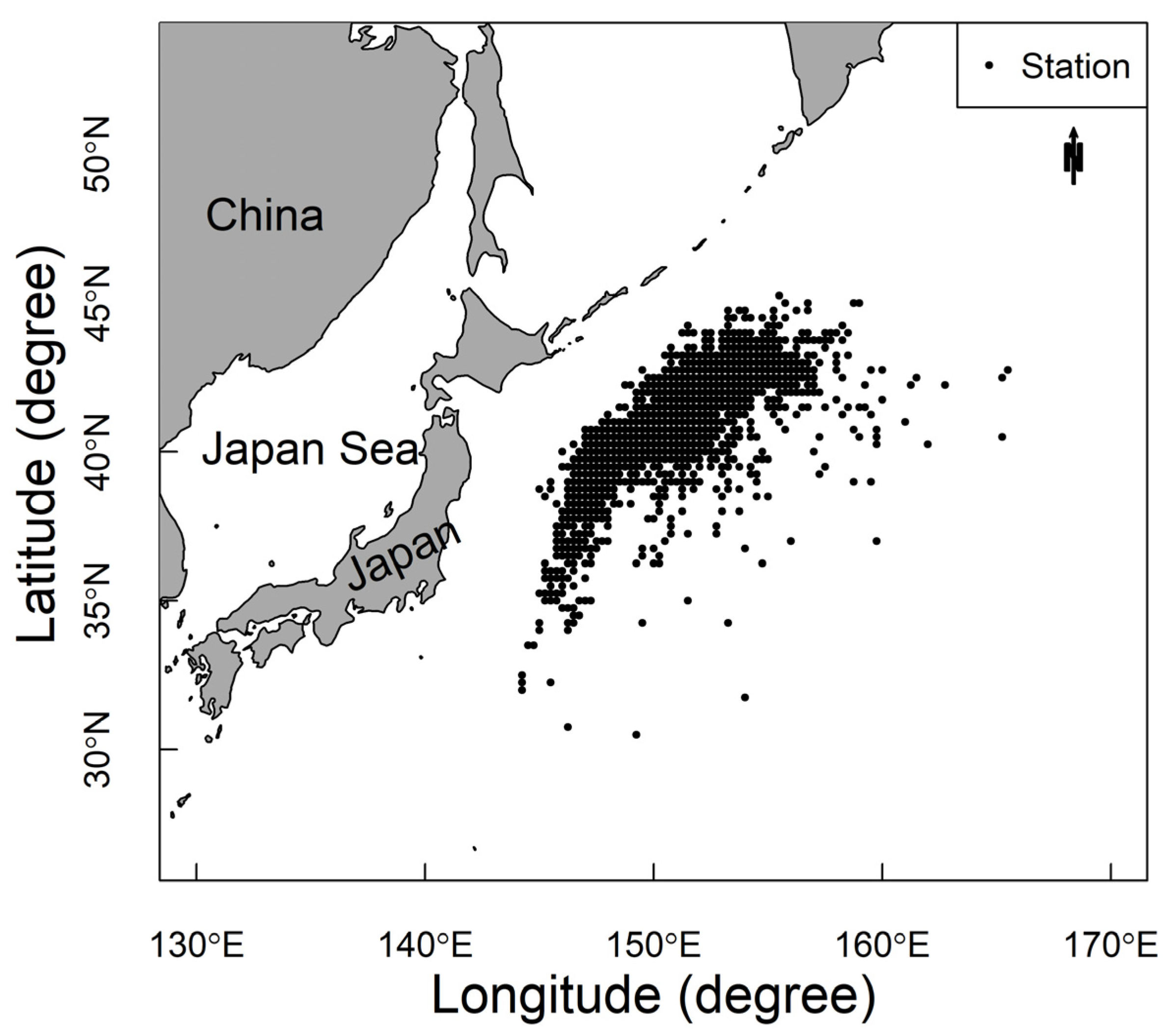
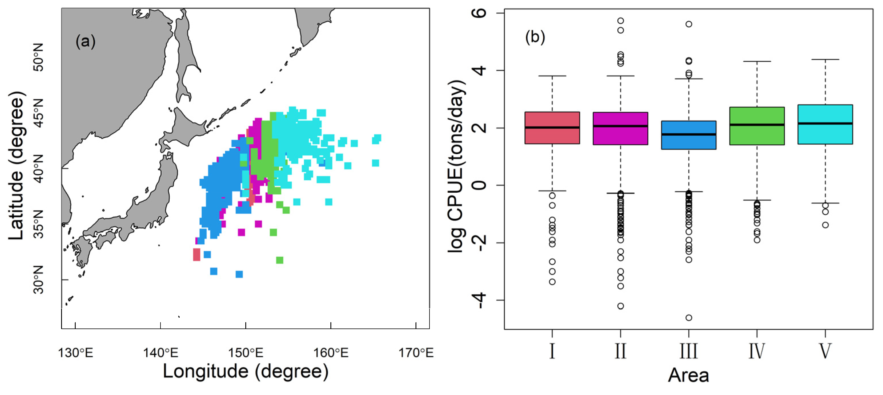
2.1. Data Sources

Figure 1 shows the research region, encompassing the geographical range between 30° N and 45° N latitude and between 143° E and 165° E longitude, and the study focuses on the primary fishing season, which occurs from May to November, from 2014 to 2021. The fishery logbook data, acquired from the Technical Group for Trawl-purse seine Fishery within the Distant-water Fishery Society of China, included information on date, longitude, latitude, catch, hauls, and vessel length, with the location data having a spatial resolution of 0.25°. No zero catches were included in the dataset (removed approximately 1% of zero catch data), and the daily vessel catch defined the nominal CPUE.

Based on the references, we selected SST(°C), SSH (m), and SSTG (°C/km) as the environmental factors when constructing the model for Pacific sardines. The SST and SSH, featuring a monthly temporal resolution and a spatial resolution of 0.25°, were acquired from the Copernicus Marine Service. This access took place on the 23rd of November 2022. The SST and SSH are the monthly average values for this grid. Regarding the SSTG, which signifies the temperature change across the ocean surface, it can influence the distribution and behavior of fish species. Additionally, it may affect the distribution of planktonic organisms, thereby impacting the food sources of fish and other marine organisms. Therefore, this environmental factor needs to be taken into account in CPUE standardization. In this study, it represents temperature variations within a 0.25° × 0.25° grid [31]. The variance inflation factor (VIF) measures the degree of multicollinearity among explanatory variables in a regression analysis, which assesses how much the variance of an estimated regression coefficient is inflated due to multicollinearity in the model. The VIF numbers represent the extent to which multicollinearity inflates the variance of the estimated regression coefficients: the larger the value, the higher the degree. According to the VIF test (

Table 1. Explanatory variables test.

Explanatory Variables	Year	Area	Vessel	SST	SSTG	SSH
VIF	1.02	1.01	1.02	1.18	1.06	1.16

), we found that there is no multicollinearity among the explanatory variables [32,33].

In this study, all data processing and model construction were conducted using R (V4.0.3). “Spatial 1”, introduced by Hsu et al. [34], was selected as the area stratification approach for the GLM and the GLMM. Using spatial proximity and average CPUE as the criteria, Spatial 1 employed the k-medoids algorithm to divide the Pacific sardine CPUE grids into five area strata. (Figure 2) [35]. Briefly, the k-medoids algorithm clusters dataset observations into k groups, each led by a representative observation (called a “medoid”). It selects these medoids by minimizing distances within clusters, ensuring every data point connects to its closest medoid. This method, using actual observations as the cluster centers, enhances its resilience to outliers. For more details on the method of partitioning area strata, please refer to Hsu et al. [34] and Ono et al. [35].

2.2. Methods

2.2.1. General Linear Models

The GLM is the most common modeling approach for CPUE standardization, assuming a linear relationship between the response variable and the explanatory factors [36]. In this study, in addition to the explanatory variables shown in Table 1, interaction terms for year and spatial location were also considered for inclusion in the GLM. Ln(CPUE) is the response variable; so, assuming that the response variable follows a normal distribution, the GLM model is as follows:

$$\mathit{Ln}\left({CPUE}_i\right)={\alpha }_{Year\left(i\right)}+{\alpha }_{Area\left(i\right)}+{\alpha }_{Vessel\left(i\right)}+{\alpha }_{SST\left(i\right)}{SST}_i+{\alpha }_{SSTG\left(i\right)}{SSTG}_i+{{\alpha }_{SSH\left(i\right)}SSH}_i+{\alpha }_{Year\left(i\right)\times Area\left(i\right)}$$

(1)

where ${CPUE}_i$ is the predicted CPUE for the ith data, and α denotes the estimated coefficient associated with its respective subscript. In the GLM, the year, area, vessel, and year × area were treated as discrete variables, and the SST, SSTG, and SSH were continuous.

2.2.2. Generalized Linear Mixed Models

The GLMM is a commonly employed model that integrates the advantages of both the GLM and the LMM, finding extensive application in CPUE standardization studies [37]. The GLMM is an extension of the GLM model that allows for the inclusion of random variables in the linear predictor for CPUE standardization [38,39]. We fit the GLMM for Pacific sardine CPUE standardization as defined by the equation presented below:

$$\mathit{Ln}\left({CPUE}_i\right)={\beta }_{Year\left(i\right)}+{\beta }_{Area\left(i\right)}+{\beta }_{Vessel\left(i\right)}+{{\beta }_{SST\left(i\right)}SST}_i+{\beta }_{SSTG\left(i\right)}{SSTG}_i+{{\beta }_{SSH\left(i\right)}SSH}_i+{\beta }_{Year\left(i\right)\times Area\left(i\right)}{Year}_i\times {Area}_i$$

(2)

where ${CPUE}_i$ represents the predicted CPUE for the ith data, and β denotes the estimated coefficient associated with its respective subscript. We consider year, area, SST, SSTG, and SSH as fixed effects, and treat the other variables as random effects in the GLMM.

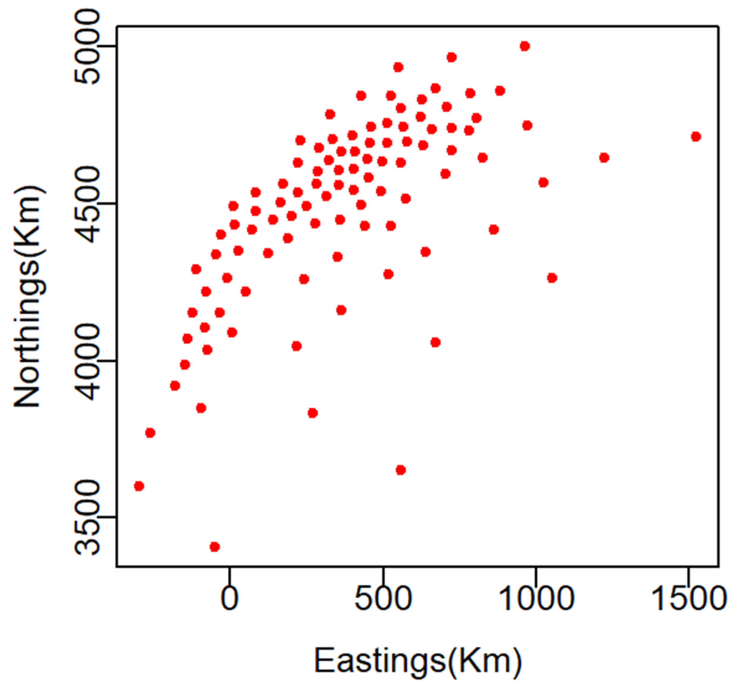
2.2.3. Spatio-Temporal GLMM (VAST)

For our spatio-temporal modeling, the VAST R package (version 3.4.0) was applied. VAST’s default model framework is founded on a delta-generalized linear mixed model, which separates the catch probability distribution into the following two discrete elements: the probability of encounter and the positive catch rate. Since there were no instances of zero CPUE data in the Pacific sardine dataset, we exclusively considered the positive catch rate component and assigned an encounter probability of one for all the years. We employed a lognormal GLMM to estimate the positive catch rate, utilizing linear predictors and a log-link function. The model also incorporated Gaussian Markov random fields (GMRFs) to effectively capture and consider both spatial and spatio-temporal effects [40].

It is necessary to define spatial knots in advance for computational convenience in the VAST. To evaluate correlations for both the spatial and spatio-temporal effects, we utilized the K-means algorithm to partition all the grid cells into 100 spatial knots, which served as reference points (Figure 3). Furthermore, the spatial and spatio-temporal random effects of each grid cell were assumed to originate from the cell’s nearest spatial knot [41], and the formula of the CPUE for Pacific sardine using logarithms is detailed as follows:

$$\mathrm{l}\mathrm{o}\mathrm{g}\left(p_i\right)=\beta \left(t_i\right)+\omega \left(s_i\right)+\epsilon \left(s_i,t_i\right)+\delta \left(v_i\right)+\sum _{j=1}^n\gamma \left(j\right)X\left(s_i,t_i,j\right)$$

(3)

where $p_i$ is the predicted CPUE of the ith data; the intercept for year $t_i$, denoted as $\beta \left(t_i\right)$, is considered a fixed effect and is assumed to be independent across various years; $\omega \left(s_i\right)$ and $\epsilon \left(s_i,t_i\right)$ are time-invariant spatial variances in location $s_i$ and time-varying spatio-temporal variances for location $s_i$ in year $t_i$, respectively. $\delta \left(v_i\right)$represents the influence of vessel $v_i,$ and $\delta \left(v_i\right)~\mathrm{N}\mathrm{o}\mathrm{r}\mathrm{m}\mathrm{a}\mathrm{l}\left(0,1\right)$, $\gamma \left(j\right)$ is the jth catchability covariate $X\left(s_i,t_i,j\right)$ on location $s_i$ during year $t_i$, and the variable n represents the total number of catchability covariates.

We applied the Laplace approximation as implemented in the Template Model Builder for parameter estimation [42]. This technique facilitated the integration of random-effect parameters and the derivation of the marginal likelihood of fixed-effect parameters. These fixed-effect parameters were subsequently estimated using a maximum likelihood estimation within the R computing environment.

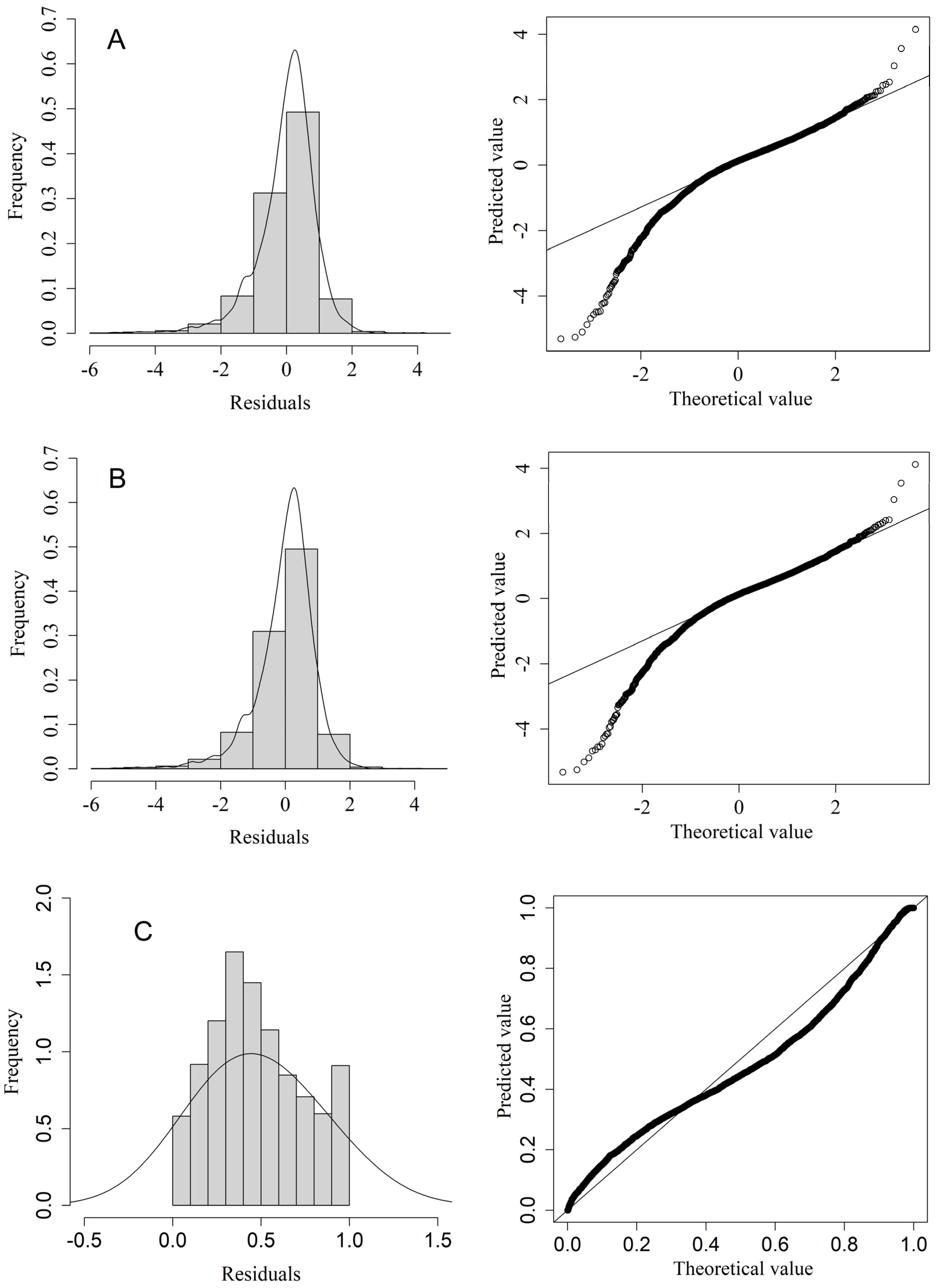
2.2.4. Model Evaluation

In the process of identifying the most suitable models among the GLM, GLMM, and VAST, we employed a forward approach by incrementally incorporating explanatory variables into each of the three models. This led to the creation of models with varying sets of explanatory variables. Subsequently, we utilized the Akaike Information Criterion (AIC) to make the final selections for the optimal GLM, GLMM, and VAST. AIC values are indicative of a model’s fit, with smaller values suggesting superior-fitting models.

To compare the performance of different models, the conditional R² and conditional AIC (CAIC) were employed, since those metrics provide a more accurate measure of model complexity [43,44]. An enhanced model performance in a standardized context is indicated with a higher conditional R² and a lower CAIC value. The CAIC formula is given below:

$$CAIC=-2ln\left(L\right)+kln\left(n\right)$$

(4)

where L denotes the value of likelihood function. In addition, we assessed the normality of the GLM, GLMM, and VAST using histograms of the residuals and quantile–quantile normal probability plots (Q-Q plots).

2.2.5. Standardized CPUE Value

Using the optimal models chosen for the three models, we computed the standardized abundance indices, and we employed the “predict” function to estimate the CPUE for the GLM and GLMM models. Following that, we utilized the aggregate function to calculate the CPUE for each year and area (${CPUE}_{Year,Area}$). Lastly, we determined the area-weighted annual CPUE using the formula below:

$${\widehat{CPUE}}_{Year}=\sum _{Area=1}^n{SA}_{Area}\times {CPUE}_{Year,Area}$$

(5)

where n represents the total number of areas, which amounts to five. The term ${SA}_{Area}$ denotes the proportion of the study domain’s surface area allocated to a particular area.

Utilizing the VAST model, which includes an explicit spatial correlation component, we estimated the Pacific sardine density in every spatial cell across the study region. The description of the standardized abundance indices for the study area in year t is as follows:

$${\widehat{CPUE}}_t=\sum _{s=1}^n{SA}_s\times exp\left(\beta \left(t\right)+\omega \left(s\right)+\epsilon \left(s,t\right)+\delta \left(v\right)+\sum _{j=1}^n\gamma \left(j\right)X\left(s_i,t_i,j\right)\right)$$

(6)

where n refers to the number of knots denoted as s; $\beta \left(t\right)$ is the year-specific effect at time t; $\omega \left(s\right)$ signifies the spatial effect at knot s, and $\epsilon \left(s,t\right)$ stands for the spatio-temporal effect at knot s during time t. Additionally, SA_s represents the surface area associated with the mesh corresponding to knot s.

2.2.6. The Impact of Predictor Variables on Standardized CPUE

In this study, we calculated the influence value for each variable. Subsequently, we generated coefficient–distribution–influence (CDI) plots, which encompass coefficient values, changes in distributions, and annual impacts [30]. These CDI plots served as a valuable resource for gaining a deeper understanding of the annual influence patterns.

To measure the extent of influence, we determined the normalized coefficient (ρ) associated with each explanatory variable using the formula below:

$$\rho ={\sum }_{i=1}^n{a}_i/n$$

(7)

where $a_i$ signifies the anticipated coefficient associated with the ith observation, and n is the overall number of CPUE observations.

Calculating the influence value (${AI}_y$) for a variable in a specific year involves finding the average difference between the coefficients linked to all the observations within that year and the normalized coefficient in a multiplicative GLMM.

$${\delta }_y=\frac{\sum _{i=1}^m{a}_i-\rho }{m}$$

(8)

where m represents the number of observations during year y. Given that the log-link function was utilized, the ${AI}_y$ was calculated using the subsequent formula:

$${AI}_y=\mathrm{e}\mathrm{x}\mathrm{p}\left({\delta }_y\right)$$

(9)

As referenced in Bentley et al. [30], when the value of ${AI}_y$ for a variable is larger than one, it signifies the variable’s contribution to an increase in the nominal CPUE for that year. Conversely, if the value is below one, it implies the opposite, and an ${AI}_y$ of one reveals that the variable had no discernible impact on the difference between the nominal and standardized CPUE.

The formula for computing the average influence metric $\overline{AI}$ for a variable across all years is as follows:

$$\overline{AI}=\mathrm{e}\mathrm{x}\mathrm{p}\left(\frac{\sum _{y=1}^m{\delta }_y}{m}\right)-1$$

(10)

where m signifies the number of years under consideration in the analysis.

We employed the year × spatial interaction random-effect CDI plot format, following the guidance of Bentley et al. [30], for creating CDI plots in both the GLM and GLMM. For the VAST, the initial set of 100 spatial knots was initially classified into 20 groups, referred to as “grouped” knots, based on the coefficients of the spatio-temporal random effect, and for more details, please refer to Hsu et al. [34].

2.2.7. Simulation Testing for Three Models

Simulation testing is a valuable tool for assessing the effectiveness of CPUE standardization models in predicting “true” abundance trends [45,46]. We established a simulation testing framework under a preferential sampling scenario [47]. Utilizing simulated data for Pacific sardines, we applied the three models to standardized CPUE data. Following that, we conducted a comparison between the models’ estimated CPUE values and the “true” values as part of the assessment of the models’ performance. For a more comprehensive understanding of the way to calculate the “true” values of CPUE and the preferential sampling pattern, we recommend consulting the research conducted by Hsu et al. [34] and Thorson et al. [10].

To assess the models’ performance, we employed a comparison of the computed indices with area weightings against the “true” indices. The evaluation criteria included the use of the relative error metric in year y (${RE}_y$), the root mean squared error (RMSE), and the bias metric ($\beta$).

The formula for calculating ${RE}_y$ is as follows:

$${RE}_y=\frac{\left(\widehat{I_y}-T_y\right)}{T_y}$$

(11)

where $\widehat{I_y}$represents the estimated CPUE during year y, and $T_y$represents the true CPUE during year y.

The calculation of the RMSE was performed according to the formula provided by Ducharme-Barth et al. [47], as follows:

$$RMSE=\sqrt{\frac{\sum _{y=1}^n{\left(\widehat{I_y}-T_y\right)}^2}{n}}$$

(12)

where n is the total count of years.

Based on the research by Thorson et al. [10] and Ducharme-Barth et al. [47], the bias metric, denoted as coefficient β, was applied in the linear model as follows:

$$\widehat{I_y}=\alpha +\beta \times T_y+{\epsilon }_y$$

(13)

$${\epsilon }_y\sim Normal\left(0,{\sigma }_{\epsilon }^2\right)$$

(14)

where $\alpha$ is the intercept of linear model, and β is the slope to the slope parameter that relates the “true” CPUE to the estimated CPUE [48].

3. Results

3.1. Diagnostic and Selection of Three Model

Table 2. Selection process of the optimal GLM.

No.	GLM Model	AIC
1	Ln(CPUE)~Year + Area + Year: Area	9755.40
2	Ln(CPUE)~Year + Area + Year:Area + Vessel	9720.78
3	Ln(CPUE)~Year + Area + Year:Area + Vessel + SST	9722.72
4	Ln(CPUE)~Year + Area + Year:Area + Vessel + SST + SSTG	9708.86
5	Ln(CPUE)~Year + Area + Year:Area + Vessel + SST + SSTG + SSH	9710.58

,

Table 3. Selection process of the optimal GLMM.

No.	GLMM Model	AIC
1	Ln(CPUE)~Year + Area + Year: Area	9795.28
2	Ln(CPUE)~Year + Area + Year:Area + Vessel	9765.51
3	Ln(CPUE)~Year + Area + Year:Area + Vessel + SST	9776.61
4	Ln(CPUE)~Year + Area + Year:Area + Vessel + SST + SSTG	9761.08
5	Ln(CPUE)~Year + Area + Year:Area + Vessel + SST + SSTG + SSH	9765.23

and

Table 4. Selection process of the optimal VAST.

No.	Covariates	AIC
1	None	8789.27
2	SST	8782.16
3	SST + SSTG	8785.38
4	SST + SSTG + SSH	8787.45

illustrate the model decision process for the three models based on the AIC criterion. The values of the AIC suggest that the most effective models for the GLM and the GLMM incorporate the following explanatory factors: year, area, vessel, SST, SSTG, and Year × Area (Table 2 and Table 3). As for the VAST, the favored model includes only the covariate SST (Table 4). Compared to the GLM and the GLMM, the VAST exhibits a higher conditional R² and smaller CAIC values (

Table 5. Summary of the three models fitted to Pacific sardine CPUE from 2014 to 2021.

Model	Conditional R2	CAIC
GLM	0.27	9709.18
GLMM	0.32	9690.90
VAST	0.36	8776.27

). Additionally, the histogram of the residuals and Q-Q plots of the three models, which are based on lognormal distributions, demonstrate normality, affirming the appropriateness of the assumption regarding the error distribution for the CPUE standardization in the three models (Figure 4).

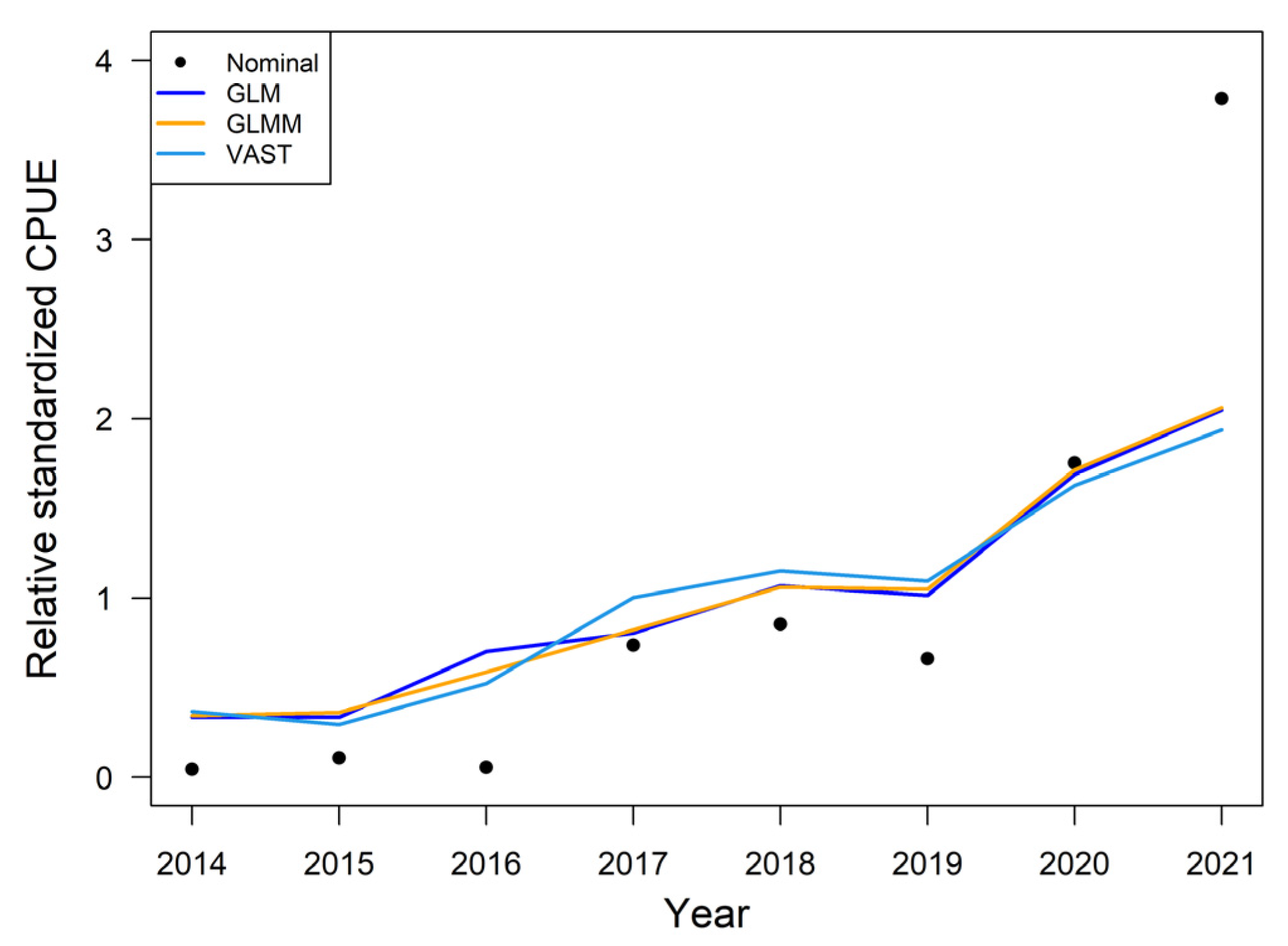
3.2. The Nominal and Standardized CPUE

An overall upward pattern was noted in both the nominal and the standardized CPUE for Pacific sardine from 2014 to 2021 (Figure 5). Except for 2015 and 2016, the relative standardized CPUE with area weightings of the three models exhibited a similar trend compared to the nominal CPUE. Specifically, the standardized CPUE showed a slight decrease from 2014 to 2015. Subsequently, from 2015 to 2018, it increased annually, followed by a decrease in 2019, and, from 2019 to 2021, there was a substantial growth in the standardized CPUE (Figure 5). Furthermore, regarding the CPUE values, except for 2020 and 2021, the standardized CPUE values of all three models were higher than the nominal CPUE. Notably, in 2021, the nominal CPUE (3.79) was significantly higher than the standardized CPUE values of the three models (GLM: 2.05, GLMM: 2.06, and VAST: 1.94).

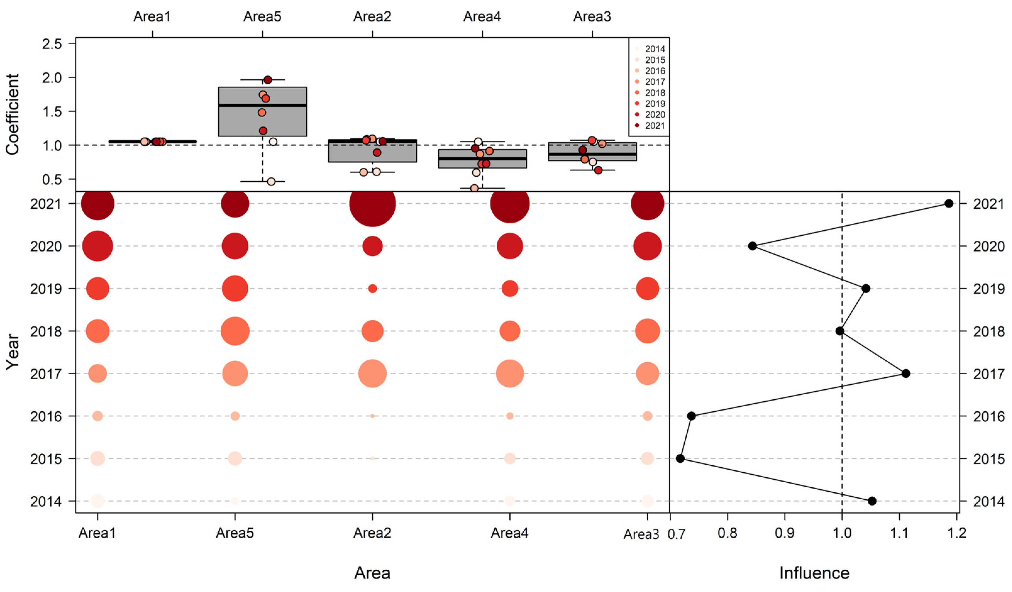
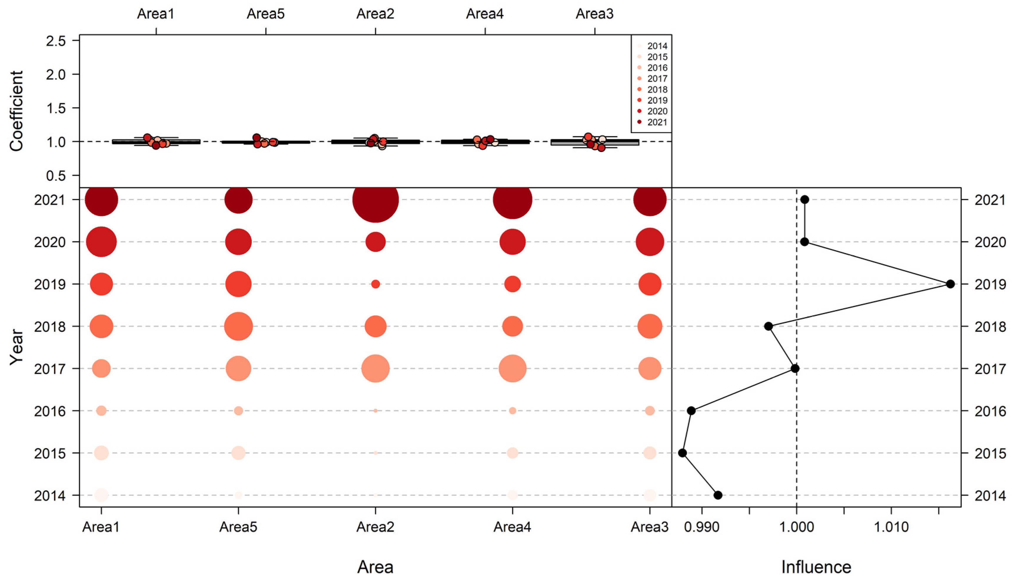
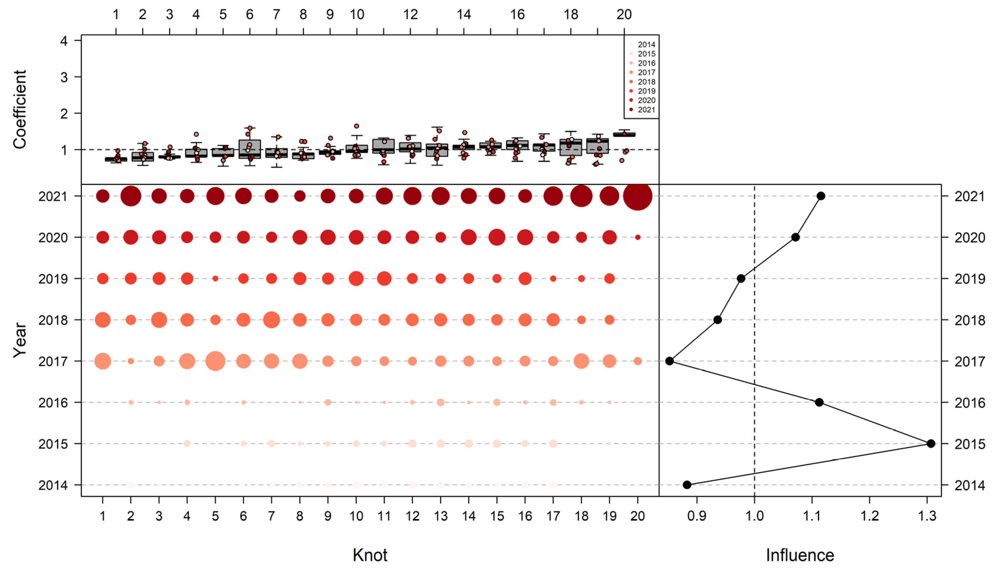
3.3. Influence of Explanatory Variables

Figure 6 depicts the annual influence plots of the explanatory variables. The spatial, year × spatial, and vessel annual influence values exhibit diverse patterns across the various models (Figure 6A–C), whereas the SST’s values consistently follow a similar trend across all the models (Figure 6D). This highlights the crucial role of model selection in CPUE standardization. In contrast to the GLMM and the VAST, the GLM demonstrates a wider spectrum of variation in annual influence, indicating that the GLMM and the VAST are more stable than the GLM in CPUE standardization. The annual relative standardized CPUE of Pacific sardine was higher than the nominal CPUE from 2014 to 2019 (Figure 5), which can be attributed to the fact that the annual influence values of the year × spatial and vessel were mainly below one in the corresponding years. However, the annual influence of the explanatory variables consistently exceeded a value of one from 2019 to 2021, resulting in standardized CPUE values lower than the nominal CPUE. The annual influence of the SST in all three models was concentrated around one, indicating that the effect of the SST on the difference between the standardized and nominal CPUE is relatively minor. Notably, the year × spatial overall influence in the GLM and the GLMM, as well as the spatio-temporal variable in the VAST, surpassed that of other variables (

Table 6. Overall influence of the three models.

Model	Variable	Overall Influence
GLM	Year	0.258
	Area	0.173
	Year × Area	0.287
	SST	0.015
GLMM	Year	0.196
	Area	0.204
	Year × Area	0.303
	SST	0.015
VAST	Year	0.217
	Area	0.209
	spatio-temporal	0.312
	SST	0.015

).

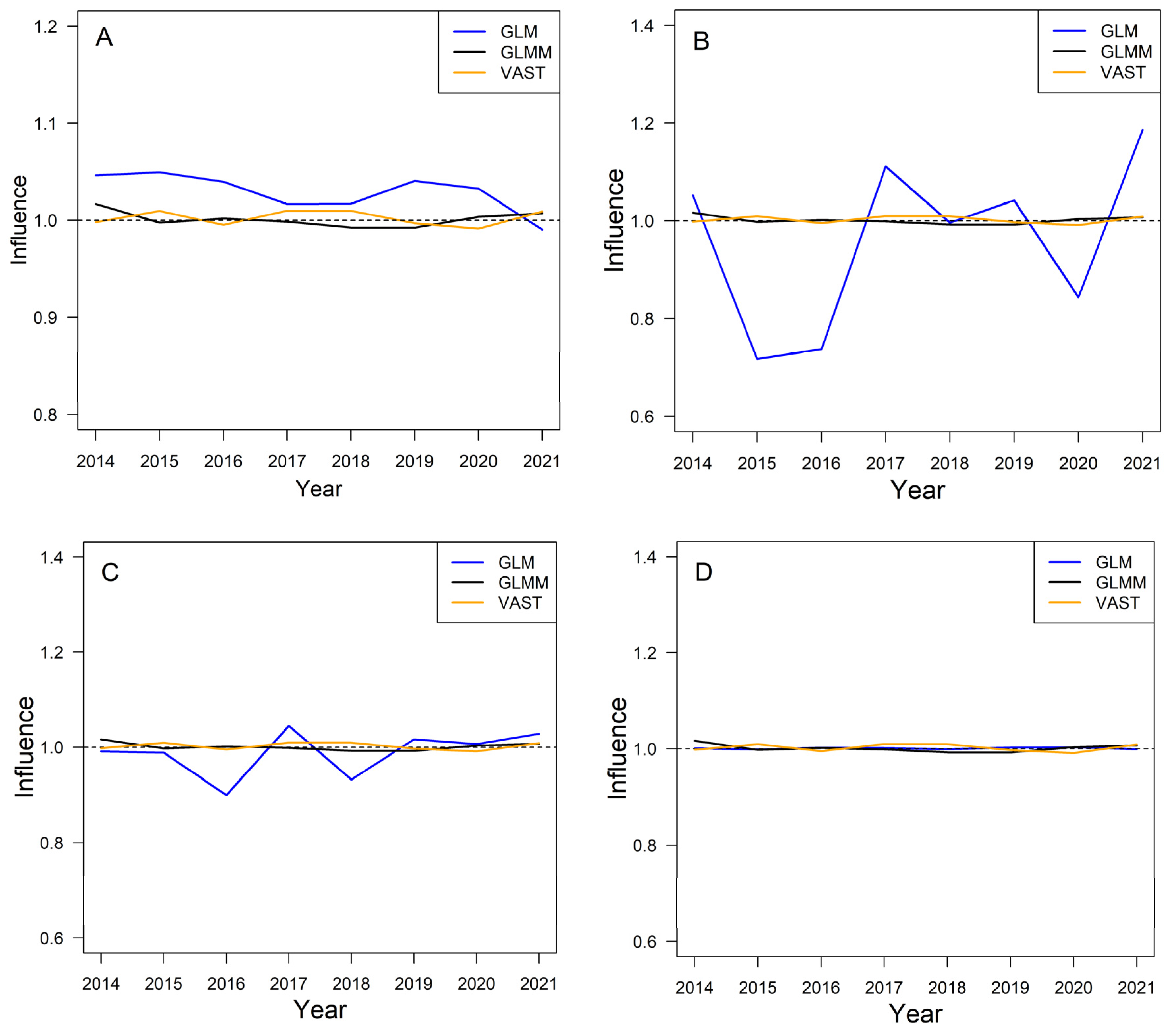
3.4. The Influence of Various Models on Yearly Standardized CPUE

Using the same data stratification method (Spatial 1), this study employed three models for CPUE standardization, allowing us to assess their impact on the standardized CPUE by examining the CDI plot of the explanatory variables. In Figure 7, the CDI plot for the year × spatial effect in the GLM is presented, and it demonstrates notable variations in the annual influence of the year × spatial (right bottom panel). More precisely, during 2015 and 2016, the values of the yearly influence were notably subdued, registering at only 0.72 and 0.74, respectively. This can be ascribed to the concentration of data primarily within areas 1, 3, and 5, where the associated coefficients are relatively modest (Figure 7). Conversely, the yearly influence value for 2021 surged to 1.19, marking a significant increase. This notable upswing is linked to the greater quantity of accessible data, primarily distributed in regions with elevated coefficients. The CDI plot illustrating the year × spatial interaction random effect in the GLMM is shown in Figure 8. Although the data distribution across the areas aligns with the GLM, the impact of the year × spatial in the GLMM model exhibits minimal variation. The lowest influence value was observed in 2015 (0.98), while the highest was observed in 2019 (1.02). This variation could be ascribed to differences in model structure between the GLM and the GLMM. Figure 9 displays the CDI plot for the spatio-temporal random effect in the VAST. In 2014 and 2017, the annual influence values remained relatively modest, primarily due to the concentration of data within knots with lower coefficients. In contrast, a higher annual influence value in 2015 was associated with the year’s elevated coefficients.

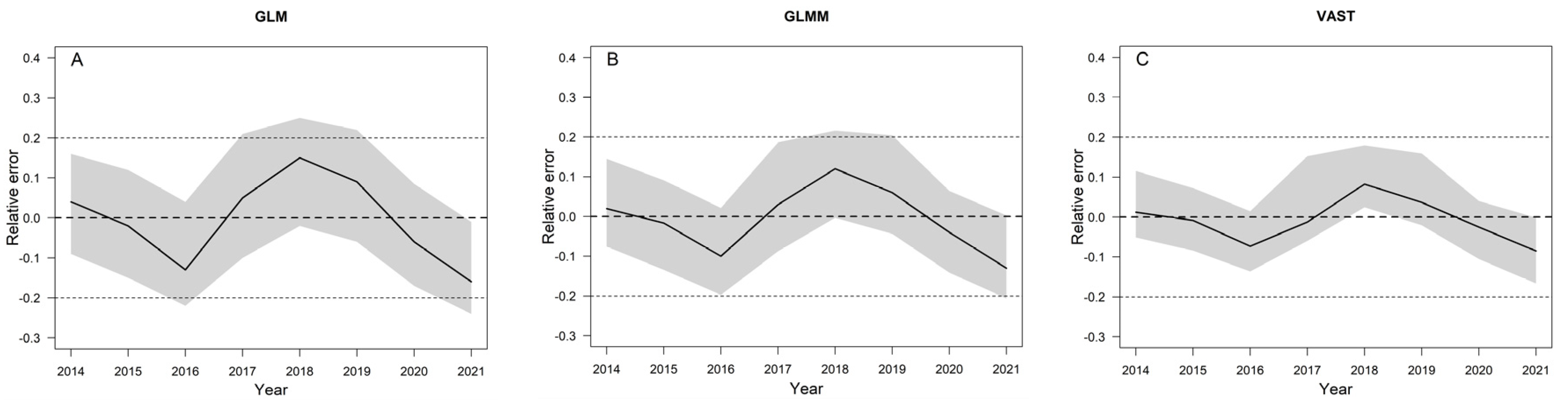
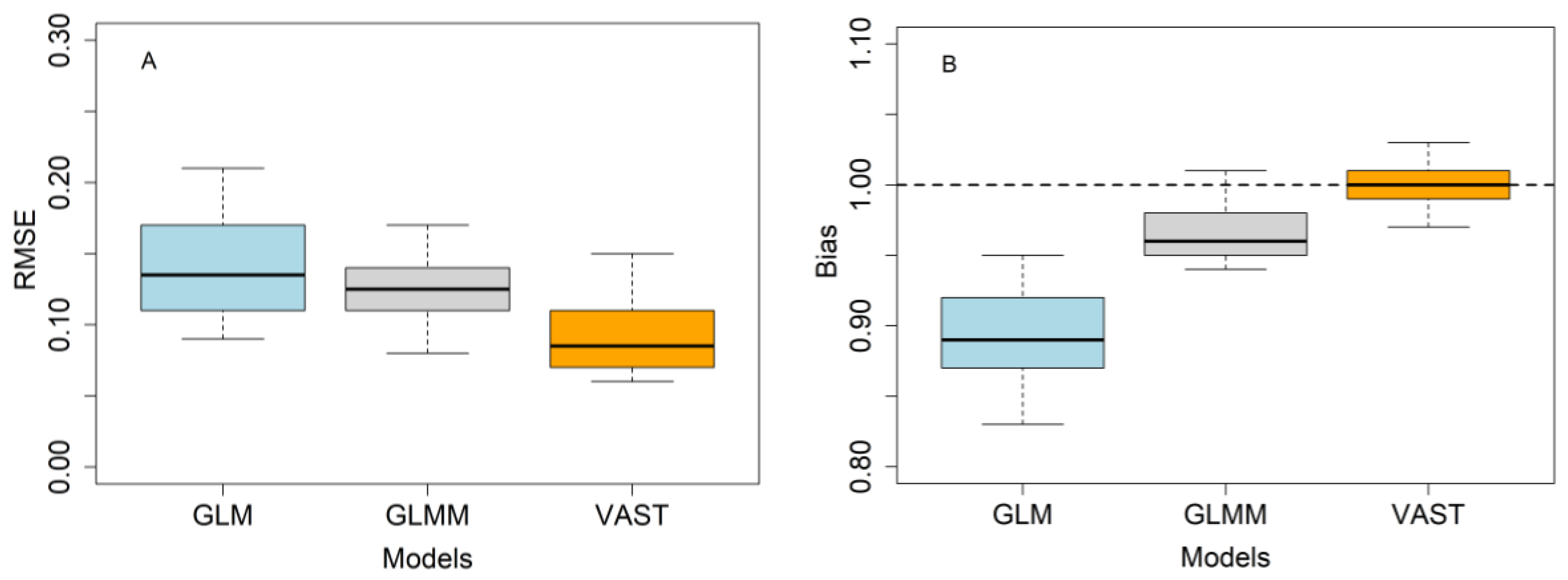
3.5. Model Evaluation Using a Simulation Test

From Figure 10, it can be observed that the VAST exhibits smaller relative errors compared to the GLM and the GLMM, and it fluctuates around the zero value, which indicates that the VAST estimates CPUE values closer to the “true” value. Among the three models, the GLM model has the most significant relative errors, followed by the GLMM model (Figure 10). Regarding the RMSE, the VAST model has the smallest RMSE value (0.093), while the GLM model has the largest value (0.143). The RMSE value for the GLMM model is 0.126 (Figure 11A). Similarly, the bias metrics values for the three models, from largest to smallest, were the GLM, the GLMM, and the VAST (Figure 11B), which suggested that the VAST model demonstrates a superior evaluation performance.

4. Discussion

Pacific sardine fishery is a traditional fishery in the NPO [49]. Since the 1990s, the catch of Pacific sardines has experienced significant fluctuations. However, after 2010, the population of Pacific sardines gradually recovered, leading to an increase in the catch. In 2021, the catch of Pacific sardines exceeded one million tons [50]. With the increase in fishing scale and economic worth, there has been a growing focus on the stock assessment and governance of Pacific sardine resources, and the NPFC has prioritized its stock assessment and management [21]. Therefore, obtaining reliable relative abundance indices is of great significance for the management of Pacific sardines. The Pacific sardine, known for its short life cycle and highly migratory behavior, demonstrates continuous fluctuations in abundance and availability that are influenced by biotic and abiotic environmental factors, exhibiting a spatial structure [51]. Hence, including spatial autocorrelation as a continuous covariate in the CPUE standardization model for Pacific sardines appears fitting. This will improve the model’s capacity to precisely grasp the spatial distinctions in the fish occurrence patterns, thus reflecting the variations more reasonably [52].

This study assessed the effectiveness of three models—the GLM, the GLMM, and the VAST—using Chinese Pacific sardine fishery data and marine environmental data including the SST, the SSTG, and the SSH. The reason for selecting the SST, the SSTG, and the SSH is that previous research has indicated that the habitat distribution and abundance of small pelagic fish species, such as the Pacific sardine, are highly sensitive to marine environmental factors, particularly the SST, the SSTG, and the SSH [53,54]. The SST has long been considered the most important influencing factor for Pacific sardine resources, and the CAIC results revealed that the best-performing GLM, GLMM, and VAST models all included the SST, confirming its significance. Nevertheless, the findings from the influence analysis revealed that the annual influence values of the SST were distributed around one (Figure 6D), suggesting that the factors affecting resource distribution might not always make a substantial contribution to the disparities between the nominal and standardized CPUE, aligning with the conclusions of Hsu et al. [34].

Based on the CAIC and the Conditional R², the VAST demonstrates a better fitting performance compared to the GLM and the GLMM (Table 5), which was consistent with the results of Kai [55]. Meanwhile, according to the simulation tests, the VAST model showed smaller RMSE and model bias, indicating that the bias values were closer to one. This suggests that the VAST model can better accommodate the spatial variations in the CPUE data and has a higher assessment accuracy. Ducharme-Barth et al. [47] conducted simulation tests on the VAST model for CPUE standardization and reached conclusions consistent with our study. This can be ascribed to three primary factors. To begin with, the VAST model encompasses both spatial and temporal data variations, accounting for spatial correlations between sampling locations and temporal correlations across different time intervals, and allows for a more accurate representation of the complex spatio-temporal patterns in the data [56]. Additionally, by introducing spatial and temporal random effects, the VAST can effectively handle the inherent correlations and disparities within the CPUE data [57]. Lastly, the VAST provides the flexibility to incorporate supplementary covariates that elucidate the fluctuations in CPUE. This helps in capturing the impacts of pertinent environmental factors and other significant variables on the standardized CPUE, facilitating a thorough and precise analysis [58].

From Figure 5, it can be observed that the values of the standardized CPUE surpassed the nominal CPUE between 2014 and 2019. However, in 2020 and 2021, the opposite trend was observed. This may be due to the fact that the values of the influence of the year × spatial or spatio-temporal variables were mostly below one from 2014 to 2019, whereas, in the following two years, their influence values exceeded one. This also demonstrates the importance of this explanatory variable in influencing the disparities between the nominal and standardized CPUE [30]. The yearly relative standardized CPUE shows a progressive upward trend between 2014 and 2021 (Figure 5), indicating the gradual recovery of Pacific sardine resources. This pattern corresponds to the noted surge in Pacific sardine catches in China during recent years. Additionally, these research findings align with those of Yang et al. [14] and can offer valuable scientific support for the establishment or adjustment of management regulations in Pacific sardine fisheries. The objective is to strike a balance between ecological preservation and the concerns of fishers.

CPUE standardization models are applied to mitigate the confounding influences of external factors and derive an indicator that accurately reflects fish biomass [59]. Therefore, it is imperative to thoroughly scrutinize the results, instead of merely adopting the CPUE data generated using the standardization model, in order to grasp the impact of including each explanatory factor in the standardized CPUE. We conducted an influence analysis for each explanatory variable of the three models, and the results indicated that, in contrast to other explanatory variables, the influence of the SST on the disparities among the standardized and nominal CPUE is relatively minor (Figure 6). The overall influence of the year × spatial or spatio-temporal variable is the highest (Table 6), which is consistent with the results of Hsu et al. [34]. From Figure 6, it can be observed that the influence values of the explanatory variables in the VAST model fluctuate less over time, while, in the GLM and GLMM models, the influence values of explanatory variables exhibit larger fluctuations over time. This also demonstrates the robustness of CPUE standardization in the VAST model.

In this study, the spatial stratification method “Spatial 1” was employed to stratify the fishery data of Pacific sardines in the NPO [34]. The influence values of the year × spatial random effect or spatio-temporal random effect in the GLMM and VAST models were consistent with the influence criteria of the relationship between the nominal and standardized CPUE (Figure 8 and Figure 9), whereas the year × spatial effect of the GLM did not exhibit this trend (Figure 7). This discrepancy highlights the differences in the data handling capabilities among the models [60]. We also discovered that the distribution of data had a significant impact on the standardized CPUE. In instances where the data clustered in regions with high coefficients, the influence value for the respective year was relatively elevated, while it was diminished when the data dispersed across areas with low coefficients (Figure 7, Figure 8 and Figure 9). Based on the existing literature, several approaches, such as the ad hoc approach [61] and the binary recursive partitioning approach [62], can be used to determine area stratification in CPUE standardization. Therefore, it is advisable to undertake future studies to examine the influence of various fishery data stratification approaches on CPUE standardization. This will impart valuable insights, delivering scientific management recommendations to a wide audience which includes fishers, managers, and stakeholders.

Our study has provided crucial insights for the stock assessment of Pacific sardine. It has also established a spatio-temporal model framework for the CPUE standardization for other small pelagic fish species worldwide, thereby supporting the conservation and sustainable use of other fish stocks. Importantly, our study once again demonstrated the impact of the SST on the distribution and abundance of Pacific sardines. However, we also discovered that explanatory variables with a high explanatory power in CPUE standardization models may not necessarily have a significant influence on the disparities between the nominal CPUE and the standardized CPUE. Therefore, this aspect should be clarified in future research. Our study revealed that the variables of year × spatial or spatio-temporal exerted the most significant overall impact concerning the standardized CPUE, indicating their significant role in explaining the disparities between the nominal and standardized CPUE. Furthermore, it highlighted the advantages of the VAST in standardizing the CPUE for highly migratory small pelagic fish species, suggesting its incorporation as a routine CPUE standardization tool. This research will facilitate the application of accurate biomass indices in stock assessment and ultimately promote the scientific management and conservation of Pacific sardines.

5. Conclusions

We effectively developed multiple models for Pacific sardine CPUE standardization and assessed the effectiveness of three models (GLM, GLMM, and VAST). While all three models displayed parallel patterns in the standardized CPUE when compared to the nominal CPUE, the VAST method exhibited a lower CAIC and a higher conditional R², indicating a better performance in fitting and prediction. This is because the VAST has the capability to consider and address temporal and spatial correlations and disparities within the CPUE data, leading to a more precise estimation of spatial and temporal effects. The VAST with only the SST as a covariate had a smaller CAIC. Influence analysis is an effective method for comprehending how each explanatory factor affects the disparities between the nominal and standardized CPUE. We performed a quantitative assessment on how each explanatory factor influenced the optimal models for the three models. The results demonstrated that the interaction terms of the three models exert a more significant influence on the standardized CPUE. This underscores the importance of thoroughly incorporating these elements in future research on Pacific sardines in the NPO. Subsequently, we produced CDI plots representing the year × spatial interaction effect or the spatio-temporal random effect. These plots illustrated that the VAST model displays an enhanced reliability when standardizing the CPUE for Pacific sardines. Simulation testing also confirmed that the VAST model exhibits the highest accuracy (with the smallest RMSE and model bias) in CPUE standardization. This suggests that the VAST model can be considered a practical approach for CPUE standardization for this fish species. The findings presented in this study represent a significant initial stride towards the balanced conservation and eco-friendly utilization of Pacific sardine resources.

References

1. Campbell, R.A. CPUE standardisation and the construction of indices of stock abundance in a spatially varying fishery using general linear models. Fish. Res. 2004, 70, 209–227. [Google Scholar] [CrossRef]
2. Hilborn, R.; Walters, C.J. Quantitative Fisheries Stock Assessment and Management: Choice, Dynamics and Uncertainty; Chapman & Hall: New York, NY, USA, 1992; p. 570. [Google Scholar]
3. Callwood, K.A. Examining the development of a parrotfish fishery in The Bahamas: Social considerations & management implications. Glob. Ecol. Conserv. 2021, 28, e01677. [Google Scholar]
4. Harley, S.J.; Myers, R.A.; Dunn, A. Is catch-per-unit-effort proportional to abundance? Can. J. Fish. Aquat. Sci. 2001, 58, 1760–1772. [Google Scholar] [CrossRef]
5. Cao, J.; Thorson, J.T.; Richards, R.A.; Chen, Y. Spatiotemporal index standardization improves the stock assessment of northern shrimp in the Gulf of Maine. Can. J. Fsih. Aquat. Sci. 2017, 74, 1781–1793. [Google Scholar] [CrossRef]
6. Walters, C. Folly and fantasy in the analysis of spatial catch rate data. Can. J. Fish. Aquat. Sci. 2003, 60, 1433–1436. [Google Scholar] [CrossRef]
7. Li, G.; Lu, Z.W.; Cao, Y.M.; Zou, L.J.; Chen, X.J. CPUE Estimation and Standardization Based on VMS: A Case Study for Squid-Jigging Fishery in the Equatorial of Eastern Pacific Ocean. Fish 2023, 8, 2. [Google Scholar] [CrossRef]
8. Hashimoto, M.; Nishijima, S.; Yukami, R.; Watanabe, C.; Kamimura, Y.; Furuichi, S.; Ichinokawa, M.; Okamura, H. Spatiotemporal dynamics of the Pacific chub mackerel revealed by standardized abundance indices. Fish. Res. 2019, 219, 105315. [Google Scholar] [CrossRef]
9. Hazin, H.G.; Hazin, F.; Mourato, B.; Carvalho, F.; Frédou, T. Standardized catch rates of swordfish (Xiphias gladius) caught by the Brazilian fleet (1978–2012) using generalized linear mixed models (GLMM) using delta log approach. Collect. Vol. Sci. Pap. ICCAT. 2014, 70, 1875–1884. [Google Scholar]
10. Thorson, J.T.; Shelton, A.O.; Ward, E.J.; Skaug, H.J. Geostatistical delta-generalized linear mixed models improve precision for estimated abundance indices for West Coast groundfishes. ICES J. Mar. Sci. 2015, 72, 1297–1310. [Google Scholar] [CrossRef]
11. Maunder, M.N.; Punt, A.E. Standardizing catch and effort data: A review of recent approaches. Fish. Res. 2004, 70, 141–159. [Google Scholar] [CrossRef]
12. Rodriguez, M.E.; Arrizabalaga, H.; Ortiz, M.; Rodriguez, C.C.; Moreno, G.; Kell, L.T. Standardization of bluefin tuna (Thurmus thynnus) catch per unit effort in the bait boat fishery of the Bay of Biscay (Eastern Atlantic). ICES J. Mar. Sci. 2003, 60, 1216–1231. [Google Scholar] [CrossRef]
13. Cortes, G.G.; Montanez, J.A.D.A.; Sánchez, F.A.; Salas, S.; Balart, E.F. How do environmental factors affect the stock–recruitment relationship? The case of the Pacific sardine (Sardinops sagax) of the northeastern Pacific Ocean. Fish. Res. 2010, 102, 173–183. [Google Scholar] [CrossRef]
14. Yang, C.; Han, H.B.; Zhang, H.; Shi, Y.C.; Su, B.; Jiang, P.W.; Xiang, D.L.; Sun, Y.Y.; Li, Y. Assessment and management recommendations for the status of Japanese sardine Sardinops melanostictus population in the Northwest Pacific. Ecol. Indic. 2023, 148, 110111. [Google Scholar] [CrossRef]
15. Tameishi, H.; Shinomiya, H.; Aoki, I.; Sugimoto, T. Understanding Japanese sardine migrations using acoustic and other aids. ICES J. Mar. Sci. 1996, 53, 167–171. [Google Scholar] [CrossRef]
16. Sarr, O.; Kindong, R.; Tian, S.Q. Knowledge on the Biological and Fisheries Aspects of the Japanese Sardine, Sardinops melanostictus (Schlegel, 1846). J. Mar. Sci. Eng. 2021, 9, 1403. [Google Scholar] [CrossRef]
17. Furuichi, S.; Niino, Y.; Kamimura, Y.; Yukami, R. Time-varying relationships between early growth rate and recruitment in Japanese sardine. Fish. Res. 2020, 232, 105723. [Google Scholar] [CrossRef]
18. FAO. FAO Yearbook; Fishery and Aquaculture Statistics: Rome, Italy, 2021; p. 13. [Google Scholar]
19. Shi, Y.C.; Zhang, X.M.; He, Y.R.; Fan, W.; Tang, F.H. Stock Assessment Using Length-Based Bayesian Evaluation Method for Three Small Pelagic Species in the Northwest Pacific Ocean. Front. Mar. Sci. 2022, 9, 775180. [Google Scholar] [CrossRef]
20. Zhao, G.Q.; Shi, Y.C.; Fan, W.; Cui, X.S.; Tang, F.H. Study on main catch composition and fishing ground change of light purse seine in Northwest Pacific. S. China Fish. Sci. 2022, 18, 33–42, (In Chinese with English Abstract). [Google Scholar]
21. North Pacific Fisheries Commission. NPFC Yearbook 2017; North Pacific Fisheries Commission: Tokyo, Japan, 2017; p. 385. Available online: www.npfc.int (accessed on 21 November 2017).
22. Shi, Y.C.; Kang, B.; Fan, W.; Xu, L.L.; Zhang, S.M.; Cui, X.S.; Dai, Y. Spatio-Temporal Variations in the Potential Habitat Distribution of Pacific Sardine (Sardinops sagax) in the Northwest Pacific Ocean. Fish 2023, 8, 86. [Google Scholar] [CrossRef]
23. Takasuka, A.; Oozeki, Y.; Aoki, I. Optimal growth temperature hypothesis: Why do anchovy flourish and sardine collapse or vice versa under the same ocean regime? Can. J. Fish. Aquat. Sci. 2007, 64, 768–776. [Google Scholar] [CrossRef]
24. Ito, S. Fishery biology of the sardine, Sardinops melanosticta (T. & S.), in the waters around Japan. Bull. Jpn. Sea Reg. Fish. Res. Lab. 1961, 9, 1–227, (In Japanese with English abstract). [Google Scholar]
25. Wada, T.; Jacobson, L.D. Regimes and stock-recruitment relationships in Japanese sardine (Sardinops melanostictus), 1951–1995. Can. J. Fish. Aquat. Sci. 1998, 55, 2455–2463. [Google Scholar] [CrossRef]
26. Matsuyama, M.; Adachi, S.; Nagahama, Y.; Kitajima, C.; Matsuura, M.S. Annual reproductive cycle of the captive female Japanese sardine (Sardinops melanostictus): Relationship to ovarian development and serum levels of gonadal steroid hormones. J. Mar. Biol. 1991, 108, 21–29. [Google Scholar] [CrossRef]
27. Nyuji, M.; Hongo, Y.; Yoneda, M.; Nakamura, M. Transcriptome characterization of BPG axis and expression profiles of ovarian steroidogenesis-related genes in the Japanese sardine. BMC Genom. 2020, 21, 668. [Google Scholar] [CrossRef] [PubMed]
28. Muko, S.; Ohshimo, S.; Kurota, H.; Yasuda, T.; Fukuwaka, M.A. Long-term distribution changes in distribution of Japanese sardine in the Sea of Japan during the stock fluctuations. Mar. Ecol. Prog. Ser. 2018, 593, 141–154. [Google Scholar] [CrossRef]
29. Sakamoto, T.; Komatsu, K.; Shirai, K.; Higuchi, T.; Ishimura, T.; Setou, T.; Kamimura, Y.; Watanabe, C.; Kawabata, A. Combining microvolume isotope analysis and numerical simulation to reproduce fish migration history. Methods Ecol. Evol. 2019, 10, 59–69. [Google Scholar] [CrossRef]
30. Bentley, N.; Kendrick, T.H.; Starr, P.J.; Breen, P.A. Influence plots and metrics: Tools for better understanding fisheries catch-per-unit-effort standardizations. ICES J. Mar. Sci. 2012, 69, 84–88. [Google Scholar] [CrossRef]
31. Howell, E.A.; Kobayashi, D.R. El Niño effects in the Palmyra Atoll region: Oceanographic changes and bigeye tuna (Thunnusobesus) catch rate variability. Fish. Oceanogr. 2006, 15, 477–489. [Google Scholar] [CrossRef]
32. Graham, M.H. Confronting multicollinearity in ecological multiple regression. Ecology 2003, 84, 2809–2815. [Google Scholar] [CrossRef]
33. Tien, B.D.; Lofman, O.; Revhaug, I.; Dick, O. Landslide susceptibility analysis in the Hoa Binh province of Vietnam using statistical index and logistic regression. Nat. Hazards 2011, 59, 1413–1444. [Google Scholar]
34. Hsu, J.; Chang, Y.J.; Ducharme-Barth, N.D. Evaluation of the influence of spatial treatments on catch-per-unit-effort standardization: A fishery application and simulation study of Pacific saury in the Northwestern Pacific Ocean. Fish. Res. 2022, 255, 106440. [Google Scholar] [CrossRef]
35. Ono, K.; Punt, A.E.; Hilborn, R. Think outside the grids: An objective approach to define spatial strata for catch and effort analysis. Fish. Res. 2015, 170, 89–101. [Google Scholar] [CrossRef]
36. Tian, S.Q.; Chen, X.J. Impacts of different calculating methods for nominal CPUE on CPUE standardization. J. Shanghai Ocean Univ. 2010, 19, 240–245. [Google Scholar]
37. Pinheiro, J.C.; Bates, D.M. Linear mixed-effects models: Basic concepts and examples. In Mixed-Effects Models in S and S-Plus; Springer: Berlin/Heidelberg, Germany, 2000; pp. 3–56. [Google Scholar]
38. Mikkonen, S.; Rahikainen, M.; Virtanen, J.; Lehtonen, R.; Kuikka, S.; Ahvonen, A. A linear mixed model with temporal covariance structures in modelling catch per unit effort of Baltic herring. ICES J. Mar. Sci. 2008, 65, 1645–1654. [Google Scholar] [CrossRef]
39. Forrestal, F.C.; Schirripa, M.; Goodyear, C.P.; Arrizabalaga, H.; Babcock, E.A.; Coelho, R.; Ingram, W.; Lauretta, M.; Ortiz, M.; Sharma, R. Testing robustness of CPUE standardization and inclusion of environmental variables with simulated longline catch datasets. Fish. Res. 2019, 210, 1–13. [Google Scholar] [CrossRef]
40. Sculley, M.L.; Brodziak, J. Quantifying the distribution of swordfish (Xiphias gladius) density in the Hawaii-based longline fishery. Fish. Res. 2020, 230, 105638. [Google Scholar] [CrossRef]
41. Grüss, A.; Walter III, J.F.; Babcock, E.A.; Forrestal, F.C.; Thorson, J.T.; Lauretta, M.V.; Schirripa, M.J. Evaluation of the impacts of different treatments of spatio-temporal variation in catch-per-unit-effort standardization models. Fish. Res. 2019, 213, 75–93. [Google Scholar] [CrossRef]
42. Kristensen, K.; Nielsen, A.; Berg, C.W.; Skaug, H.; Bell, B. TMB: Automatic Differentiation and Laplace Approximation. J. Stat. Softw. 2016, 70, 1–21. [Google Scholar] [CrossRef]
43. Greven, S.; Kneib, T. On the behaviour of marginal and conditional AIC in linear mixed models. Biometrika 2010, 97, 773–789. [Google Scholar] [CrossRef]
44. Nakagawa, S.; Schielzeth, H. A general and simple method for obtaining R2 from generalized linear mixed-effects models. Methods Ecol. Evol. 2013, 4, 133–142. [Google Scholar] [CrossRef]
45. Carruthers, T.R.; Li, C.J.; McAllister, M.K. Assessing methods for detecting marine ecosystem regime shifts: A simulation test. Fish. Res. 2004, 67, 173–187. [Google Scholar]
46. Methratta, E.T.; Link, J.S.; Dow, D.M. Simulation testing of stock assessment models. Fish. Res. 2003, 65, 253–264. [Google Scholar]
47. Ducharme-Barth, N.D.; Grüss, A.; Vincent, M.T.; Kiyofuji, H.; Aoki, Y.; Pilling, G.; Hampton, J.; Thorson, J.T. Impacts of fisheries-dependent spatial sampling patterns on catch-per-unit-effort standardization: A simulation study and fishery application. Fish. Res. 2022, 246, 106169. [Google Scholar] [CrossRef]
48. Wilberg, M.J.; Thorson, J.T.; Linton, B.C.; Berkson, J. Incorporating time-varying catchability into population dynamic stock assessment models. Rev. Fish. Sci. 2010, 18, 7–24. [Google Scholar] [CrossRef]
49. Nakai, Z. Studies relevant to mechanisms underlying the fluctuation in the catch of the Japanese sardine, Sardinops melanosticta. Jpn. J. Ichthyol. 1962, 9, 1–115. [Google Scholar]
50. Saito, R.; Oozeki, Y.; Takasaki, K.; Saito, T.; Uehara, S.; Miyahara, M. Transshipment activities in the North Pacific Fisheries Commission Convention Area. Mar. Policy 2022, 146, 105299. [Google Scholar] [CrossRef]
51. Watanabe, Y.; Zenitani, H.; Kimura, R. Population decline of the Japanese sardine Sardinops melanostictus owing to recruitment failures. Can. J. Fish. Aquat. Sci. 1995, 52, 1609–1616. [Google Scholar] [CrossRef]
52. Thorson, J.T.; Barnett, L.A. Comparing estimates of abundance trends and distribution shifts using single-and multispecies models of fishes and biogenic habitat. ICES J. Mar. Sci. 2017, 74, 1311–1321. [Google Scholar] [CrossRef]
53. Song, H.; Miller, A.J.; McClatchie, S.; Weber, E.D.; Nieto, K.M.; Checkley, D.M.J. Application of a data-assimilation model to variability of Pacific sardine spawning and survivor habitats with ENSO in the California Current System. J. Geophys. Res. 2012, 117, C03009. [Google Scholar] [CrossRef]
54. Vander, L.C.D.; Castro, L.; Drapeau, L.; Checkley, D., Jr. (Eds.) Report of a GLOBEC-SPACC Workshop on Characterizing and Comparing the Spawning Habitats of Small Pelagic Fish; GLOBEC Report 21; GLOBEC: Swindon, UK, 2005; Volume 7, p. 33. [Google Scholar]
55. Kai, M. Spatio-temporal changes in catch rates of pelagic sharks caught by Japanese research and training vessels in the western and central North Pacific. Fish. Res. 2019, 216, 177–195. [Google Scholar] [CrossRef]
56. Thorson, J.T. Guidance for decisions using the Vector Autoregressive Spatio-Temporal (VAST) package in stock, ecosystem, habitat and climate assessments. Fish. Res. 2019, 210, 143–161. [Google Scholar] [CrossRef]
57. Han, Q.P.; Shan, X.J.; Jin, X.S.; Gorfine, H. Overcoming gaps in a seasonal time series of Japanese anchovy abundance to analyse interannual trends. Ecol. Indic. 2023, 149, 110189. [Google Scholar] [CrossRef]
58. Thorson, J.T.; Adams, C.F.; Brooks, E.N.; Eisner, L.B.; Kimmel, D.G.; Legault, C.M.; Rogers, L.A.; Yasumiishi, E.M. Seasonal and interannual variation in spatio-temporal models for index standardization and phenology studies. ICES J. Mar. Sci. 2020, 77, 1879–1892. [Google Scholar] [CrossRef]
59. Quirijns, F.; Poos, J.; Rijnsdorp, A. Standardizing commercial CPUE data in monitoring stock dynamics: Accounting for targeting behaviour in mixed fisheries. Fish. Res. 2008, 89, 1–8. [Google Scholar] [CrossRef]
60. Campbell, R.A. A new spatial framework incorporating uncertain stock and fleet dynamics for estimating fish abundance. Fish Fish. Oxf. 2016, 17, 56–77. [Google Scholar] [CrossRef]
61. Nakano, H. Stock status of Pacific swordfish, Xiphias gladius, inferred from CPUE of the Japanese longline fleet standardized using general linear models. US Nat. Mar. Fish. Serv. NOAA Tech. Rep. NMFS 1998, 142, 195–209. [Google Scholar]
62. Ichinokawa, M.; Brodziak, J. Using adaptive area stratification to standardize catch rates with application to North Pacific swordfish (Xiphias gladius). Fish. Res. 2010, 106, 249–260. [Google Scholar] [CrossRef]
Figure 1. Sampling locations (black dots) of Pacific sardines in the Northwest Pacific Ocean.
Fishes 08 00606 g001
Figure 2. The distribution (a) and the boxplots of the CPUE data (b) for each area strata. The colors of each area in Figure (a) are consistent with Figure (b), i.e., the blue represents the area three. The boxes in Figure (b) represents the middle 50% of the data; the median line indicates the median of the data, the small circles is very big or small data in CPUE, and the lines extending from the box represent the data outside the box.
Fishes 08 00606 g002
Figure 3. Distribution of the 100 core knots in the VAST. The northing is the “distance traveled or measured northward, especially at sea”, and the easting is the distance traveled or measured to the east.
Fishes 08 00606 g003
Figure 4. Diagnostic plots for the optimal GLM, GLMM, and VSAT. The histogram of the residuals (left) and Q-Q plot (right) from (A) the GLM, (B) the GLMM, and (C) the VAST. The thick black lines in Q-Q plot represent the consistency between theoretical CPUE and predicted CPUE, and the circles represent abnormal data.
Fishes 08 00606 g004
Figure 5. Yearly relative nominal and standardized CPUE for the three models, all of which are calculated with area weightings.
Fishes 08 00606 g005
Figure 6. Yearly impact of explanatory factors on the standardized CPUE of Pacific sardine for the three models. (A) corresponds to the spatial effect; (B) denotes the interaction between the year and the spatial/spatio-temporal random effect; (C) represents the vessel effect, and (D) signifies the SST’s effect. The dotted lines is the reference line for each explanatory factors to judge the influence on the standardized CPUE.
Fishes 08 00606 g006
Figure 7. The CDI plot of the year × spatial interaction in the GLM analysis. The top section of the picture displays the normalized coefficients corresponding to each geographical area. Each year is represented by a solid color point indicating its coefficient. To enhance graphical visualization, a small amount of random noise was added to the area coefficient for each year. The lower left portion of picture displays bubbles that represent the yearly distribution of observed CPUE values across each area stratum. The size of each bubble corresponds to the number of data records it represents. The lower right portion of picture displays the yearly influence value of the year × spatial effect.
Fishes 08 00606 g007
Figure 8. The CDI plot of the year × spatial interaction random effect in the GLMM. The top section of the picture displays the normalized coefficients corresponding to each geographical area. Each year is represented by a solid color point indicating its coefficient. To enhance graphical visualization, a small amount of random noise was added to the area coefficient for each year. The lower left portion of picture displays bubbles that represent the yearly distribution of observed CPUE values across each area stratum. The size of each bubble corresponds to the number of data records it represents. The lower right portion of picture displays the yearly influence value of the year × spatial effect.
Fishes 08 00606 g008
Figure 9. The CDI plot of the spatio-temporal random effect in the VAST. The top section of the picture displays the normalized coefficients corresponding to each geographical area. Each year is represented by a solid color point indicating its coefficient. To enhance graphical visualization, a small amount of random noise was added to the area coefficient for each year. The lower left portion of picture displays bubbles that represent the yearly distribution of observed CPUE values across each area stratum. The size of each bubble corresponds to the number of data records it represents. The lower right portion of picture displays the yearly influence value of the spatio-temporal effect.
Fishes 08 00606 g009
Figure 10. The relative error trends for the three models, with the 95% confidence interval depicted as a light grey polygon.
Fishes 08 00606 g010
Figure 11. RMSE and bias measures for the GLM, GLMM, and VAST models. In Figure (A) the boxes represent the RMSE of each model. In Figure (B), a horizontal dashed line serves as the reference for the bias metrics, showing that there is no bias present.
Fishes 08 00606 g011