
Does Soundpeaking Affect the Behavior of Chub (Squalius cephalus) and Brown Trout (Salmo trutta)? An Experimental Approach

 , , , , and
Abstract
1. Introduction
1.1. Hearing Capabilities in Teleost Fish
1.2. Relevance of the Underwater Soundscape for Fish
2. Material and Methods
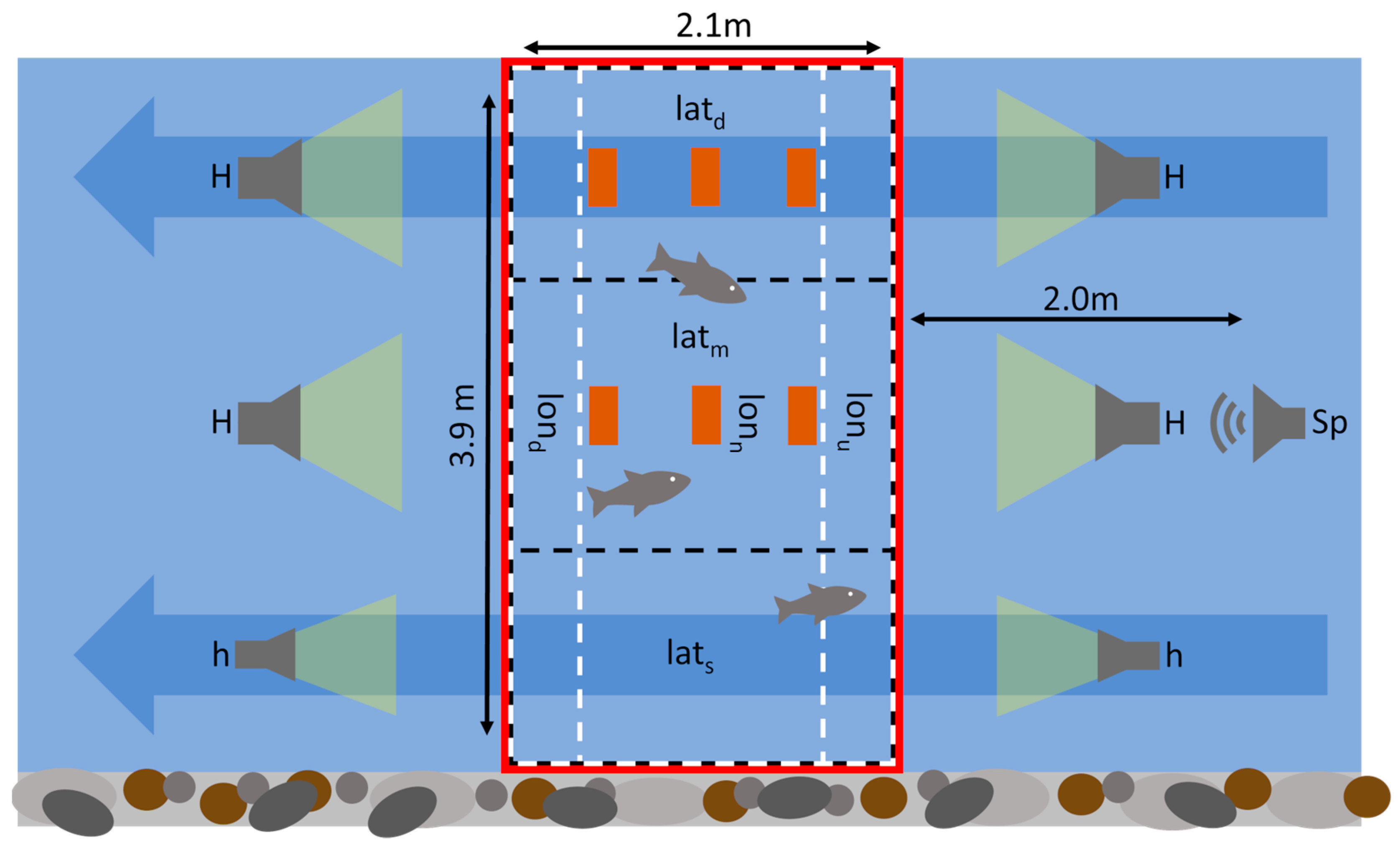
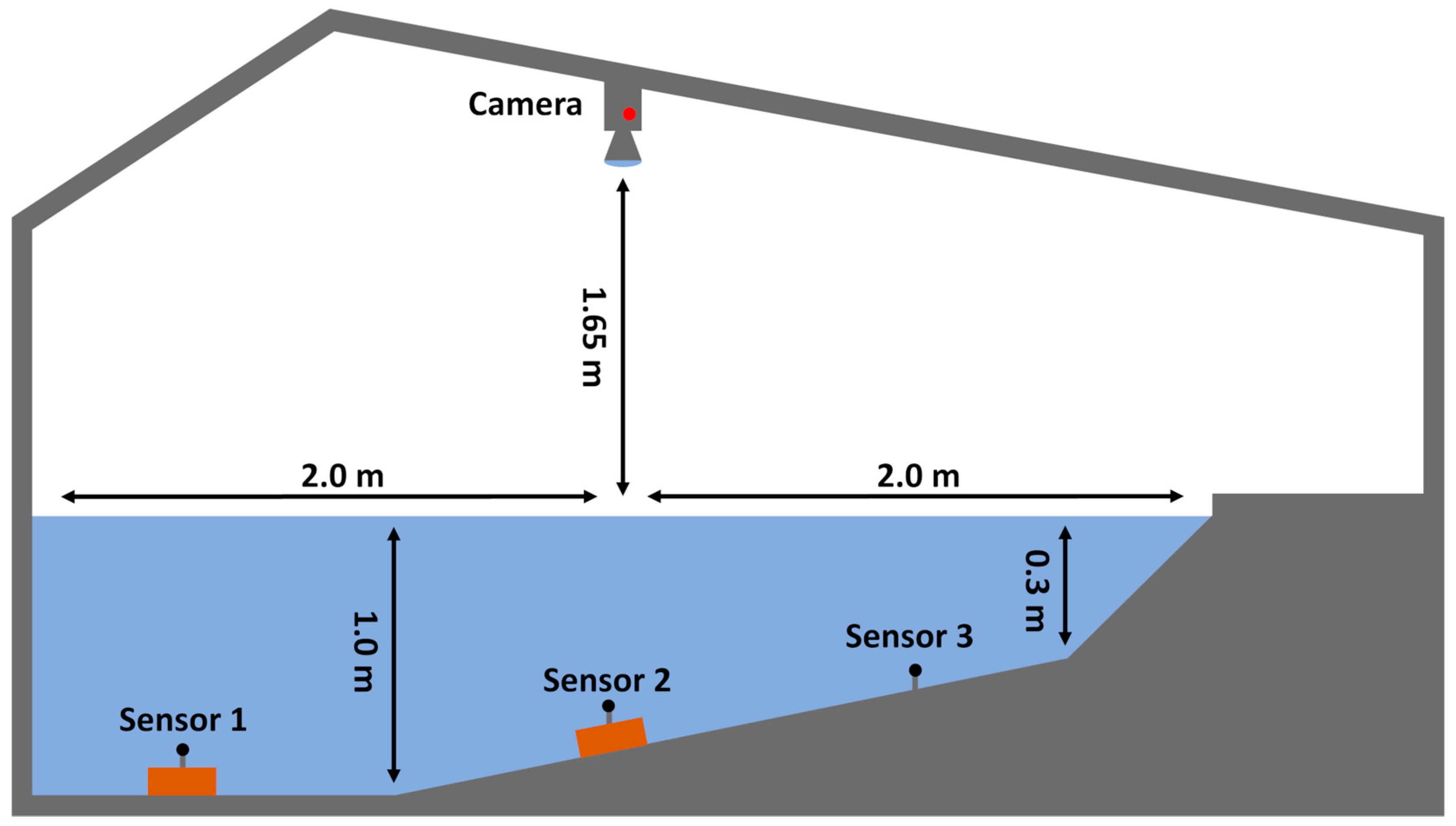
2.1. Experimental Setup and Design
2.2. Video Post-Processing and Tracking
2.3. Data Analysis
2.3.1. Variable Calculations
2.3.2. Statistical Analysis
3. Results
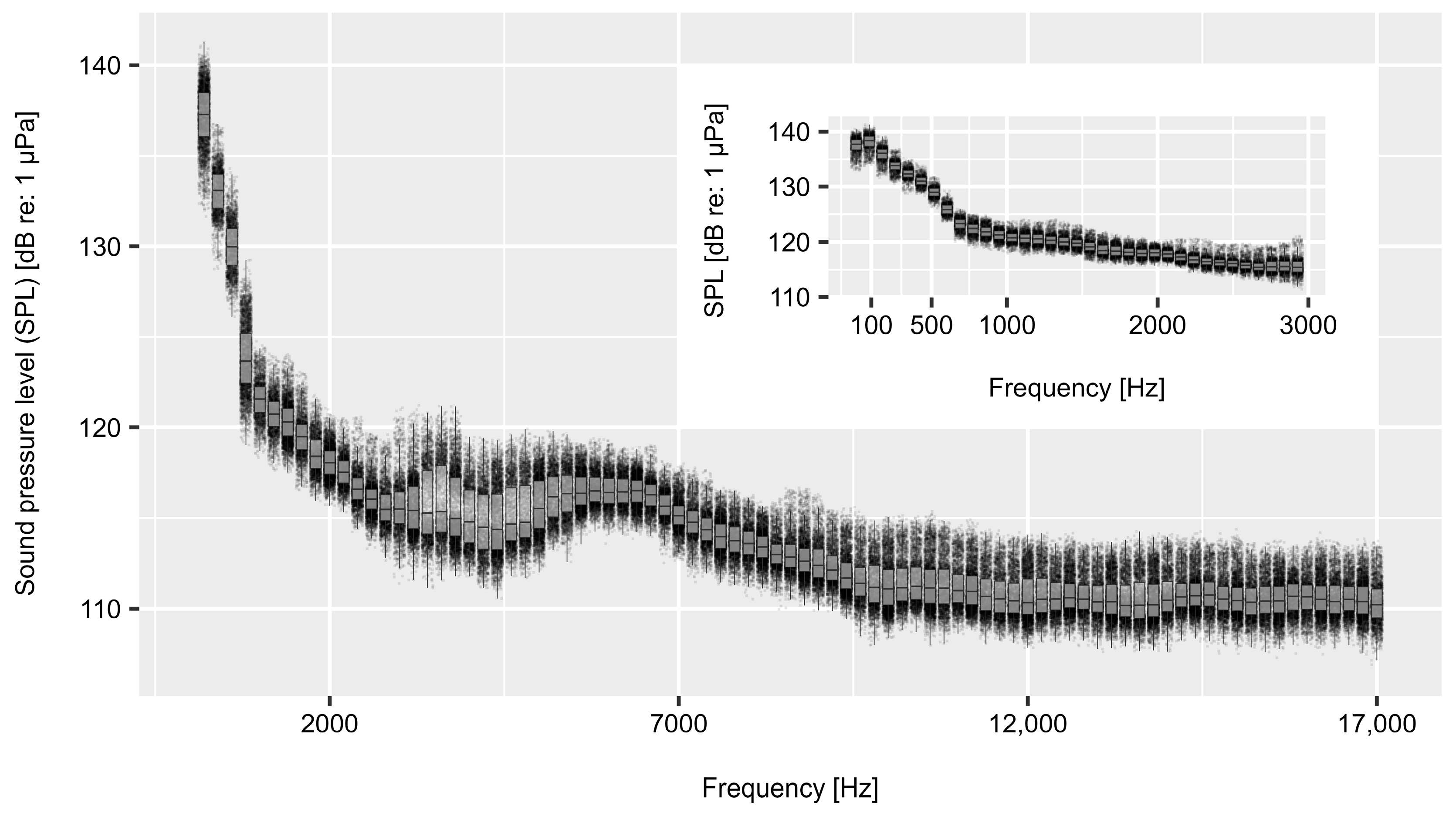
3.1. Abiotic Variables
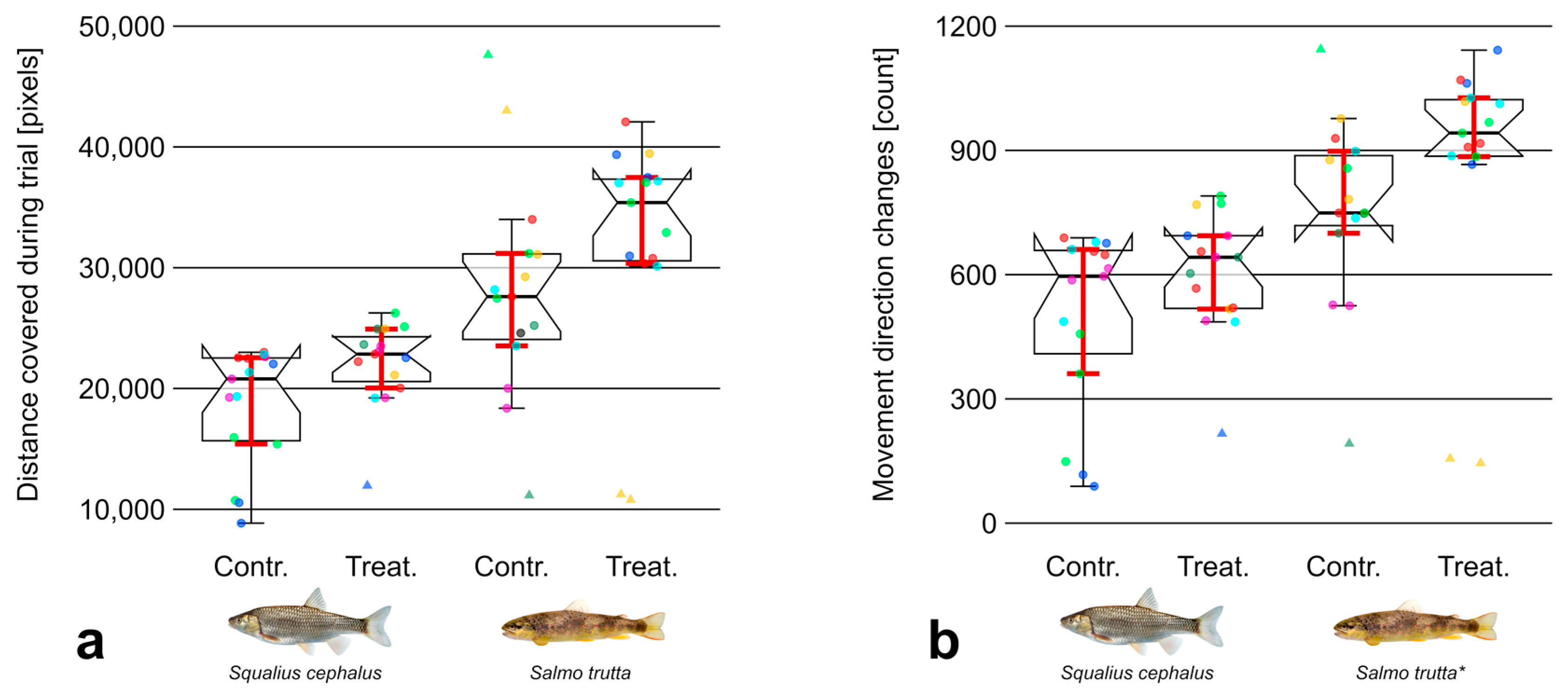
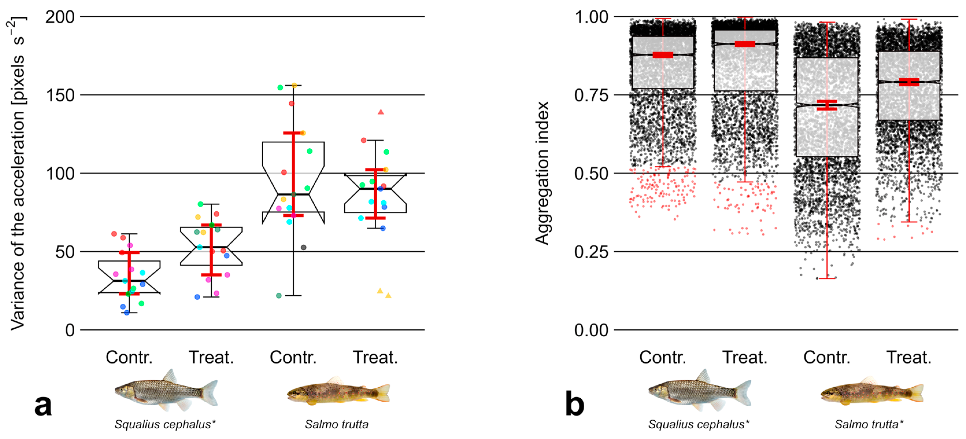
3.2. Movement
3.3. Aggregation
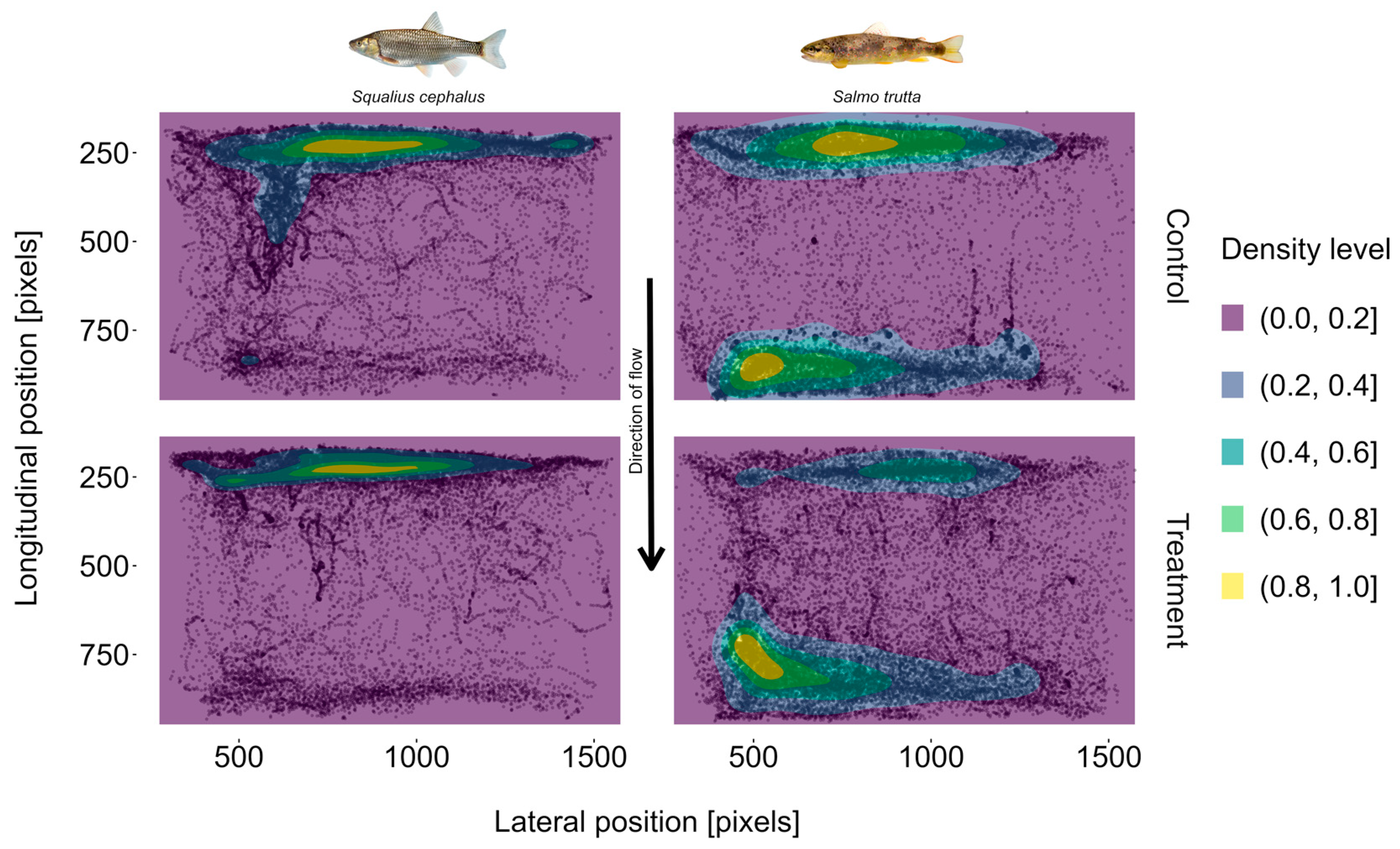
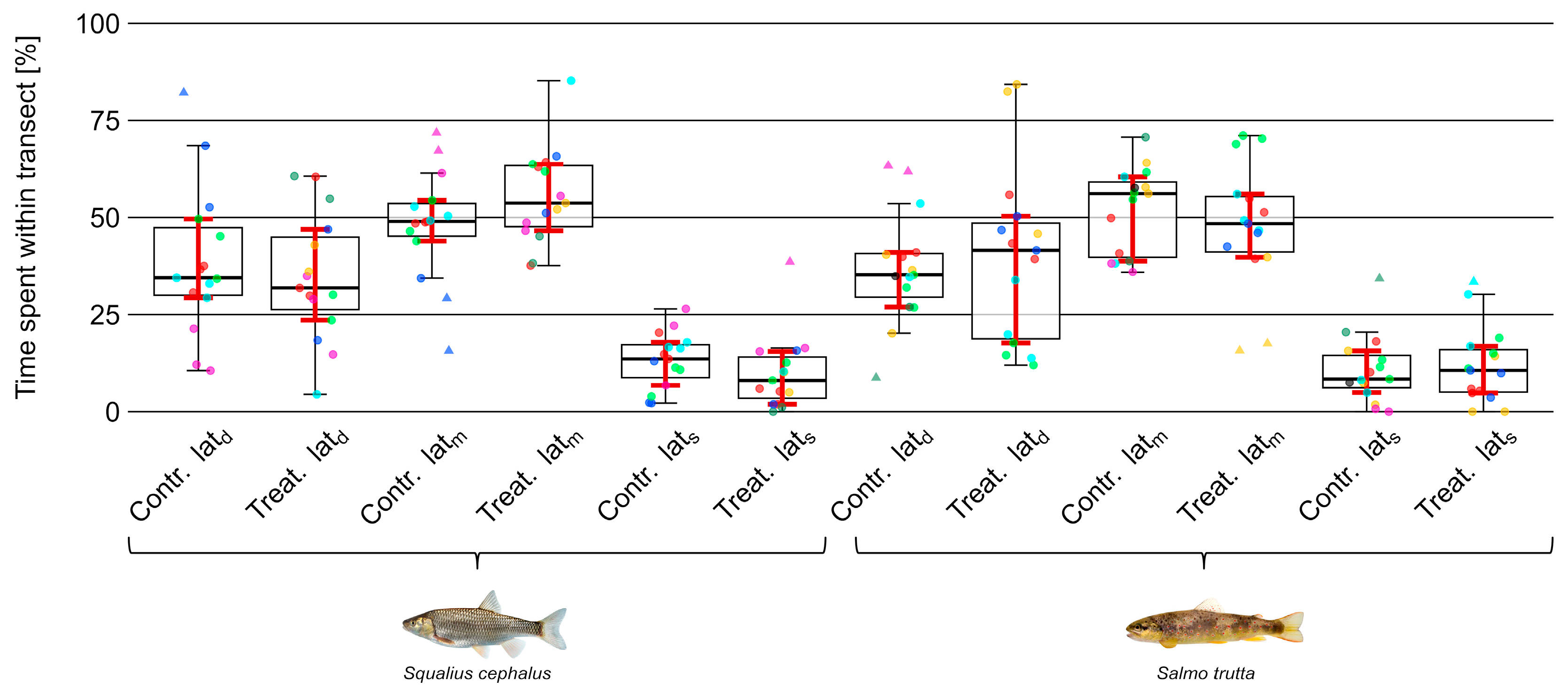
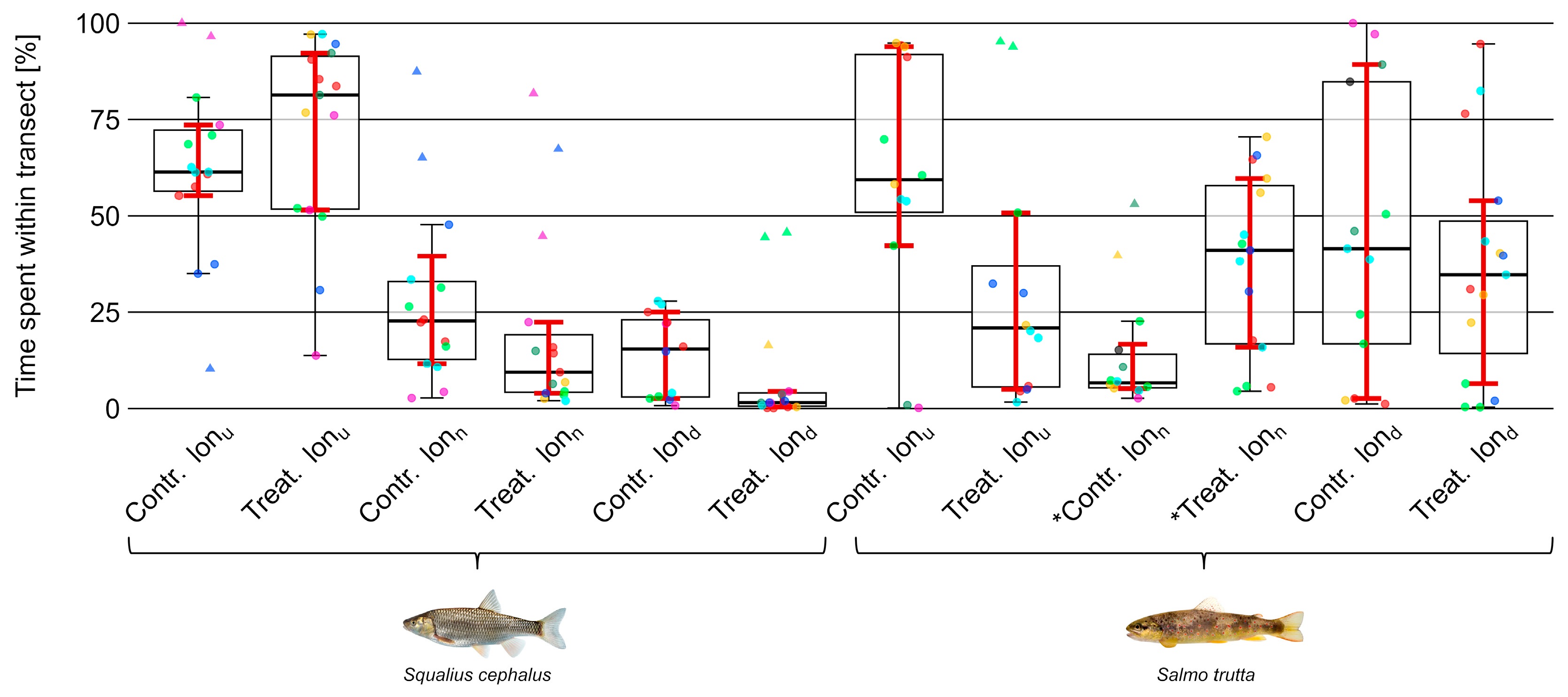
3.4. Position
4. Discussion
5. Conclusions
Author Contributions
Funding
Institutional Review Board Statement
Data Availability Statement
Acknowledgments
Conflicts of Interest
References
- Tavolga, W.N. 6 Sound Production and Detection. In Sensory Systems and Electric Organs; Elsevier: Amsterdam, The Netherlands, 1971; pp. 135–205. ISBN 9780123504050. [Google Scholar]
- Vigoureux, P. Underwater sound. Proc. R. Soc. Lond. B Biol. Sci. 1960, 152, 49–51. [Google Scholar] [CrossRef] [PubMed]
- Klaus, M.; Geibrink, E.; Hotchkiss, E.R.; Karlsson, J. Listening to air–water gas exchange in running waters. Limnol. Oceanogr. Methods 2019, 17, 395–414. [Google Scholar] [CrossRef]
- Tonolla, D.; Lorang, M.S.; Heutschi, K.; Tockner, K. A flume experiment to examine underwater sound generation by flowing water. Aquat. Sci. 2009, 71, 449–462. [Google Scholar] [CrossRef]
- Thorne, P.D. An overview of underwater sound generated by interparticle collisions and its application to the measurements of coarse sediment bedload transport. Earth Surf. Dynam. 2014, 2, 531–543. [Google Scholar] [CrossRef][Green Version]
- Tonolla, D.; Lorang, M.S.; Heutschi, K.; Gotschalk, C.C.; Tockner, K. Characterization of spatial heterogeneity in underwater soundscapes at the river segment scale. Limnol. Oceanogr. 2011, 56, 2319–2333. [Google Scholar] [CrossRef]
- Lumsdon, A.E.; Artamonov, I.; Bruno, M.C.; Righetti, M.; Tockner, K.; Tonolla, D.; Zarfl, C. Soundpeaking—Hydropeaking induced changes in river soundscapes. River Res. Appl. 2018, 34, 3–12. [Google Scholar] [CrossRef]
- Platt, C.; Popper, A.N.; Fay, R.R. The Ear as Part of the Octavolateralis System. In The Mechanosensory Lateral Line; Coombs, S., Görner, P., Münz, H., Eds.; Springer: New York, NY, USA, 1989; pp. 633–651. ISBN 978-1-4612-8157-3. [Google Scholar]
- Hawkins, A.D.; Popper, A.N. Directional hearing and sound source localization by fishes. J. Acoust. Soc. Am. 2018, 144, 3329. [Google Scholar] [CrossRef]
- Fay, R.R. The goldfish ear codes the axis of acoustic particle motion in three dimensions. Science 1984, 225, 951–954. [Google Scholar] [CrossRef]
- Popper, A.N.; Fay, R.R.; Platt, C.; Sand, O. Sound Detection Mechanisms and Capabilities of Teleost Fishes. In Sensory Processing in Aquatic Environments; Collin, S.P., Marshall, J.N., Eds.; Springer: New York, NY, USA, 2003; pp. 3–38. ISBN 978-0-387-95527-8. [Google Scholar]
- Fay, R.R. Analytic listening by the goldfish. Hear. Res. 1992, 59, 101–107. [Google Scholar] [CrossRef]
- Fay, R.R. Auditory stream segregation in goldfish (Carassius auratus). Hear. Res. 1998, 120, 69–76. [Google Scholar] [CrossRef]
- Popper, A.N.; Hawkins, A.D.; Sand, O.; Sisneros, J.A. Examining the hearing abilities of fishes. J. Acoust. Soc. Am. 2019, 146, 948. [Google Scholar] [CrossRef]
- Bird, N.C.; Hernandez, P.L. Morphological variation in the Weberian apparatus of Cypriniformes. J. Morphol. 2007, 268, 739–757. [Google Scholar] [CrossRef] [PubMed]
- Rogers, P.H.; Cox, M. Underwater Sound as a Biological Stimulus. In Sensory Biology of Aquatic Animals; Atema, J., Fay, R.R., Popper, A.N., Tavolga, W.N., Eds.; Springer: New York, NY, USA, 1988; pp. 131–149. ISBN 978-1-4612-8317-1. [Google Scholar]
- Jacobs, D.W.; Tavolga, W.N. Acoustic intensity limens in the goldfish. Anim. Behav. 1967, 15, 324–335. [Google Scholar] [CrossRef] [PubMed]
- Rüter, A. Die Anpassung der Hörschwelle von Einheimischen Fischarten an Ihre Hydroakustische Umwelt. Ph.D. Thesis, Rheinischen Friedrich-Wilhelms-Universität, Bonn, Germany, 2014. [Google Scholar]
- Hawkins, A.D.; Johnstone, A.D.F. The hearing of the Atlantic Salmon, Salmo salar. J. Fish Biol. 1978, 13, 655–673. [Google Scholar] [CrossRef]
- Harding, H. Measurement of Hearing in the Atlantic salmon (Salmo salar) using Auditory Evoked Potentials, and effects of Pile Driving Playback on salmon Behaviour and Physiology. Scott. Mar. Freshw. Sci. 2016, 7. [Google Scholar] [CrossRef]
- Johnson, M.F.; Rice, S.P. Animal perception in gravel-bed rivers: Scales of sensing and environmental controls on sensory information. Can. J. Fish. Aquat. Sci. 2014, 71, 945–957. [Google Scholar] [CrossRef]
- Melcher, A.; Hauer, C.; Zeiringer, B. Aquatic Habitat Modeling in Running Waters. In Riverine Ecosystem Management; Schmutz, S., Sendzimir, J., Eds.; Springer International Publishing: Cham, Switzerland, 2018; pp. 129–149. ISBN 978-3-319-73249-7. [Google Scholar]
- Tonolla, D.; Acuña, V.; Lorang, M.S.; Heutschi, K.; Tockner, K. A field-based investigation to examine underwater soundscapes of five common river habitats. Hydrol. Process. 2010, 24, 3146–3156. [Google Scholar] [CrossRef]
- Wohl, E.; Merritt, D.M. Reach-scale channel geometry of mountain streams. Geomorphology 2008, 93, 168–185. [Google Scholar] [CrossRef]
- Gaál, L.; Szolgay, J.; Kohnová, S.; Parajka, J.; Merz, R.; Viglione, A.; Blöschl, G. Flood timescales: Understanding the interplay of climate and catchment processes through comparative hydrology. Water Resour. Res. 2012, 48. [Google Scholar] [CrossRef]
- Rossi, T.; Nagelkerken, I.; Pistevos, J.C.A.; Connell, S.D. Lost at sea: Ocean acidification undermines larval fish orientation via altered hearing and marine soundscape modification. Biol. Lett. 2016, 12, 20150937. [Google Scholar] [CrossRef]
- Tolimieri, N.; Haine, O.; Montgomoery, J.C.; Jeffs, A. Ambient sound as a navigational cue for larval reef fish. Bioacoustics 2002, 12, 214–217. [Google Scholar] [CrossRef]
- Linke, S.; Gifford, T.; Desjonquères, C.; Tonolla, D.; Aubin, T.; Barclay, L.; Karaconstantis, C.; Kennard, M.J.; Rybak, F.; Sueur, J. Freshwater ecoacoustics as a tool for continuous ecosystem monitoring. Front. Ecol. Environ. 2018, 16, 231–238. [Google Scholar] [CrossRef]
- Amoser, S.; Ladich, F. Year-round variability of ambient noise in temperate freshwater habitats and its implications for fishes. Aquat. Sci. 2010, 72, 371–378. [Google Scholar] [CrossRef]
- Currie, H.A.L.; White, P.R.; Leighton, T.G.; Kemp, P.S. Collective behaviour of the European minnow (Phoxinus phoxinus) is influenced by signals of differing acoustic complexity. Behav. Process. 2021, 189, 104416. [Google Scholar] [CrossRef]
- Kacem, Z.; Rodríguez, M.A.; Roca, I.T.; Proulx, R. The riverscape meets the soundscape: Acoustic cues and habitat use by brook trout in a small stream. Can. J. Fish. Aquat. Sci. 2020, 77, 991–999. [Google Scholar] [CrossRef]
- Rocaspana, R.; Aparicio, E.; Palau-Ibars, A.; Guillem, R.; Alcaraz, C. Hydropeaking effects on movement patterns of brown trout (Salmo trutta L.). River Res. Applic. 2019, 35, 646–655. [Google Scholar] [CrossRef]
- Taylor, M.K.; Cooke, S.J. Meta-analyses of the effects of river flow on fish movement and activity. Environ. Rev. 2012, 20, 211–219. [Google Scholar] [CrossRef]
- Taylor, M.K.; Hasler, C.T.; Hinch, S.G.; Lewis, B.; Schmidt, D.C.; Cooke, S.J. Reach-scale movements of bull trout (Salvelinus confluentus) relative to hydropeaking operations in the Columbia River, Canada. Ecohydrology 2013, 7, 1079–1086. [Google Scholar] [CrossRef]
- Taylor, M.K.; Hasler, C.T.; Findlay, C.S.; Lewis, B.; Schmidt, D.C.; Hinch, S.G.; Cooke, S.J. Hydrologic Correlates of Bull Trout (Salvelinus confluentus) Swimming Activity in a Hydropeaking River. River Res. Appl. 2014, 30, 756–765. [Google Scholar] [CrossRef]
- Ladich, F. Ecology of sound communication in fishes. Fish Fish. 2019, 20, 552–563. [Google Scholar] [CrossRef]
- Popper, A.N.; Hawkins, A.D. An overview of fish bioacoustics and the impacts of anthropogenic sounds on fishes. J. Fish Biol. 2019, 94, 692–713. [Google Scholar] [CrossRef]
- Shafiei Sabet, S.; Wesdorp, K.; Campbell, J.; Snelderwaard, P.; Slabbekoorn, H. Behavioural responses to sound exposure in captivity by two fish species with different hearing ability. Anim. Behav. 2016, 116, 1–11. [Google Scholar] [CrossRef]
- Voellmy, I.K.; Purser, J.; Simpson, S.D.; Radford, A.N. Increased noise levels have different impacts on the anti-predator behaviour of two sympatric fish species. PLoS ONE 2014, 9, e102946. [Google Scholar] [CrossRef] [PubMed]
- Ladich, F.; Fay, R.R. Auditory evoked potential audiometry in fish. Rev. Fish Biol. Fish. 2013, 23, 317–364. [Google Scholar] [CrossRef] [PubMed]
- Provincial Government of Lower Austria. Station Number: 214262. 2021. Available online: https://www.noel.gv.at/wasserstand/#/de/Messstellen/Details/214262/Durchfluss/3Tage (accessed on 30 May 2022).
- Jackson, B.E.; Evangelista, D.J.; Ray, D.D.; Hedrick, T.L. 3D for the people: Multi-camera motion capture in the field with consumer-grade cameras and open source software. Biol. Open 2016, 5, 1334–1342. [Google Scholar] [CrossRef] [PubMed]
- Bradski, G. The OpenCV library. Version: 4.5.2. In Dr. Dobb’s Journal of Software Tools; UBM: San Francisco, CA, USA, 2000. [Google Scholar]
- R Core Team. R: A Language and Environment for Statistical Computing; R Foundation for Statistical Computing: Vienna, Austria, 2021; Available online: https://www.R-project.org/ (accessed on 20 October 2021).
- Maisog, J.M.; Wang, Y.; Luta, G.; Liu, J. Ptinpoly: Point-in-Polyhedron Test (2D and 3D). 2020. Available online: https://CRAN.R-project.org/package=ptinpoly (accessed on 31 October 2023).
- Hothorn, T.; Hornik, K.; van de Wiel, M.A.; Zeileis, A. A Lego System for Conditional Inference. Am. Stat. 2006, 60, 257–263. [Google Scholar] [CrossRef]
- Cramér, H. Mathematical Methods of Statistics; Princeton Mathematical Series; Princeton University Press: Princeton, NJ, USA, 1974; Volume 9. [Google Scholar]
- Canty, A.; Ripley, B.D. Boot: Bootstrap R (S-Plus) Functions, R Package Version 1.3-28; 2021. Available online: https://CRAN.R-project.org/package=boot (accessed on 15 November 2021).
- Davison, A.C.; Hinkley, D.V. Bootstrap Methods and Their Application; Cambridge Series on Statistical and Probabilistic Mathematics; Cambridge University Press: Cambridge, UK, 1997; Volume 1. [Google Scholar]
- Harrel, F.E.; Hmisc: Harrell Miscellaneous. R Package Version 4.6-0. 2021. Available online: https://CRAN.R-project.org/package=Hmisc (accessed on 15 November 2021).
- Martins, C.I.M.; Galhardo, L.; Noble, C.; Damsgård, B.; Spedicato, M.T.; Zupa, W.; Beauchaud, M.; Kulczykowska, E.; Massabuau, J.-C.; Carter, T.; et al. Behavioural indicators of welfare in farmed fish. Fish Physiol. Biochem. 2012, 38, 17–41. [Google Scholar] [CrossRef] [PubMed]
- Li, D.; Wang, G.; Du, L.; Zheng, Y.; Wang, Z. Recent advances in intelligent recognition methods for fish stress behavior. Aquac. Eng. 2022, 96, 102222. [Google Scholar] [CrossRef]
- Pieniazek, R.H.; Mickle, M.F.; Higgs, D.M. Comparative analysis of noise effects on wild and captive freshwater fish behaviour. Anim. Behav. 2020, 168, 129–135. [Google Scholar] [CrossRef]
- Smith, M.E.; Kane, A.S.; Popper, A.N. Noise-induced stress response and hearing loss in goldfish (Carassius auratus). J. Exp. Biol. 2004, 207, 427–435. [Google Scholar] [CrossRef]
- Greimel, F.; Schülting, L.; Graf, W.; Bondar-Kunze, E.; Auer, S.; Zeiringer, B.; Hauer, C. Hydropeaking Impacts and Mitigation. In Riverine Ecosystem Management; Schmutz, S., Sendzimir, J., Eds.; Springer International Publishing: Cham, Switzerland, 2018; pp. 91–110. ISBN 978-3-319-73249-7. [Google Scholar]
- Simpson, S.D.; Radford, A.N.; Nedelec, S.L.; Ferrari, M.C.O.; Chivers, D.P.; McCormick, M.I.; Meekan, M.G. Anthropogenic noise increases fish mortality by predation. Nat. Commun. 2016, 7, 10544. [Google Scholar] [CrossRef]
- Hanache, P.; Spataro, T.; Firmat, C.; Boyer, N.; Fonseca, P.; Médoc, V. Noise-induced reduction in the attack rate of a planktivorous freshwater fish revealed by functional response analysis. Freshw. Biol. 2020, 65, 75–85. [Google Scholar] [CrossRef]
- Auer, S.; Zeiringer, B.; Führer, S.; Tonolla, D.; Schmutz, S. Effects of river bank heterogeneity and time of day on drift and stranding of juvenile European grayling (Thymallus thymallus L.) caused by hydropeaking. Sci. Total Environ. 2017, 575, 1515–1521. [Google Scholar] [CrossRef]
- Wysocki, L.E.; Davidson, J.W.; Smith, M.E.; Frankel, A.S.; Ellison, W.T.; Mazik, P.M.; Popper, A.N.; Bebak, J. Effects of aquaculture production noise on hearing, growth, and disease resistance of rainbow trout Oncorhynchus mykiss. Aquaculture 2007, 272, 687–697. [Google Scholar] [CrossRef]
- Davidson, J.; Bebak, J.; Mazik, P. The effects of aquaculture production noise on the growth, condition factor, feed conversion, and survival of rainbow trout, Oncorhynchus mykiss. Aquaculture 2009, 288, 337–343. [Google Scholar] [CrossRef]
- Magurran, A.E.; Pitcher, T.J. Provenance, shoal size and the sociobiology of predator-evasion behaviour in minnow shoals. Proc. R. Soc. Lond. B 1987, 229, 439–465. [Google Scholar] [CrossRef]
- Schwartz, J.S.; Herricks, E.E. Fish use of stage-specific fluvial habitats as refuge patches during a flood in a low-gradient Illinois stream. Can. J. Fish. Aquat. Sci. 2005, 62, 1540–1552. [Google Scholar] [CrossRef]
- Popper, A.N.; Hawkins, A.D.; Sisneros, J.A. Fish hearing “specialization”—A re-evaluation. Hear. Res. 2022, 425, 108393. [Google Scholar] [CrossRef]
- Sadoul, B.; Geffroy, B. Measuring cortisol, the major stress hormone in fishes. J. Fish Biol. 2019, 94, 540–555. [Google Scholar] [CrossRef]
- EU. Directive of the European Parliament and of the Council of 22 September 2010 on the protection of animals used for scientific purposes. Off. J. Eur. Union 2010, 33–79. [Google Scholar]
- Kowal, J.L. Does Soundpeaking Affect the Behavior of Chub (Squalius cephalus) and Brown Trout (Salmo trutta)? Master’s Thesis, University of Natural Resources and Life Sciences, Vienna, Austria, 2022. [Google Scholar]


| ; | 16.4 | 1.0 | 543.6 | 35.0 |
| S1 | 16.4 | 1.0 | 468.4 | 33.0 |
| S2 | 16.4 | 1.0 | 628.3 | 90.7 |
| S3 | 16.3 | 1.0 | 534.2 | 89.8 |
| S4 | 16.7 | 0.9 | 12,078.8 | 10,615.5 |
Disclaimer/Publisher’s Note: The statements, opinions and data contained in all publications are solely those of the individual author(s) and contributor(s) and not of MDPI and/or the editor(s). MDPI and/or the editor(s) disclaim responsibility for any injury to people or property resulting from any ideas, methods, instructions or products referred to in the content. |
© 2023 by the authors. Licensee MDPI, Basel, Switzerland. This article is an open access article distributed under the terms and conditions of the Creative Commons Attribution (CC BY) license (https://creativecommons.org/licenses/by/4.0/).
Share and Cite
Kowal, J.L.; Auer, S.; Schmutz, S.; Graf, W.; Wimmer, R.; Tonolla, D.; Meulenbroek, P. Does Soundpeaking Affect the Behavior of Chub (Squalius cephalus) and Brown Trout (Salmo trutta)? An Experimental Approach. Fishes 2023, 8, 581. https://doi.org/10.3390/fishes8120581
Kowal JL, Auer S, Schmutz S, Graf W, Wimmer R, Tonolla D, Meulenbroek P. Does Soundpeaking Affect the Behavior of Chub (Squalius cephalus) and Brown Trout (Salmo trutta)? An Experimental Approach. Fishes. 2023; 8(12):581. https://doi.org/10.3390/fishes8120581
Chicago/Turabian StyleKowal, Johannes L., Stefan Auer, Stefan Schmutz, Wolfram Graf, Richard Wimmer, Diego Tonolla, and Paul Meulenbroek. 2023. "Does Soundpeaking Affect the Behavior of Chub (Squalius cephalus) and Brown Trout (Salmo trutta)? An Experimental Approach" Fishes 8, no. 12: 581. https://doi.org/10.3390/fishes8120581
APA StyleKowal, J. L., Auer, S., Schmutz, S., Graf, W., Wimmer, R., Tonolla, D., & Meulenbroek, P. (2023). Does Soundpeaking Affect the Behavior of Chub (Squalius cephalus) and Brown Trout (Salmo trutta)? An Experimental Approach. Fishes, 8(12), 581. https://doi.org/10.3390/fishes8120581