
Behavior Recognition of Squid Jigger Based on Deep Learning

 ,
,
Abstract
:
1. Introduction
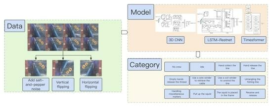
- This study first constructed a dataset on the work behaviors of squid fishing boat crew and proposed a division basis for their actions.
- This study then utilized deep learning techniques in the fisheries EMS to classify the work behaviors of crew members.
- This study, for the first time, applied the LSTM-ResNet, TimeSformer models in an offshore fishery EMS and improved the 3DCNN model used by Wang et al. in identifying whether a fishing boat is moving by imitating the ResNet model, allowing it to be applicable and maintain high accuracy on the EMS squid fishing boat crew dataset.
- Based on previous scholars’ research, this study compared the effects of commonly used 3DCNN, LSTM+ResNet, and TimeSformer models under different parameters in the field of video recognition on the EMS squid fishing boat crew dataset. The results indicate that the LSTM+ResNet model performs the best. It also provides a detailed analysis of the performance and reasons for the performance of the three models under different parameters and presents prospects for the future application of deep learning models in offshore EMS crew behavior recognition.
2. Materials and Methods
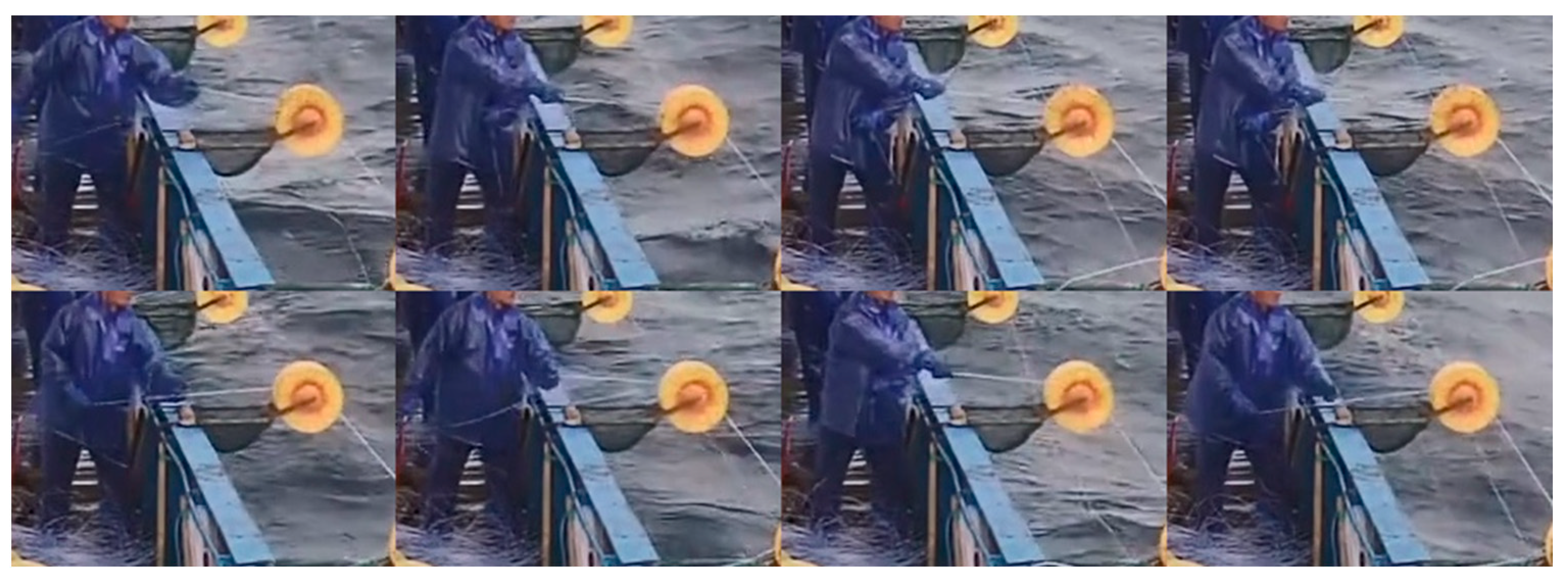
2.1. Data Collection
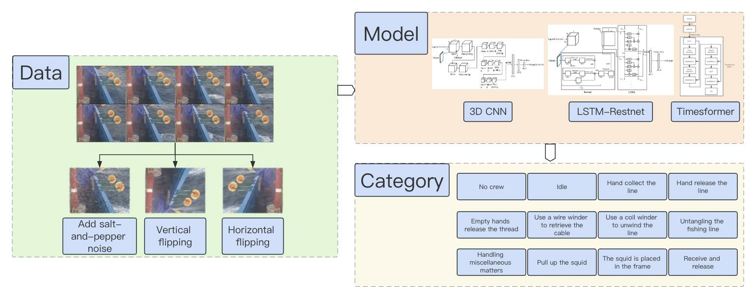
2.2. Dataset Generation
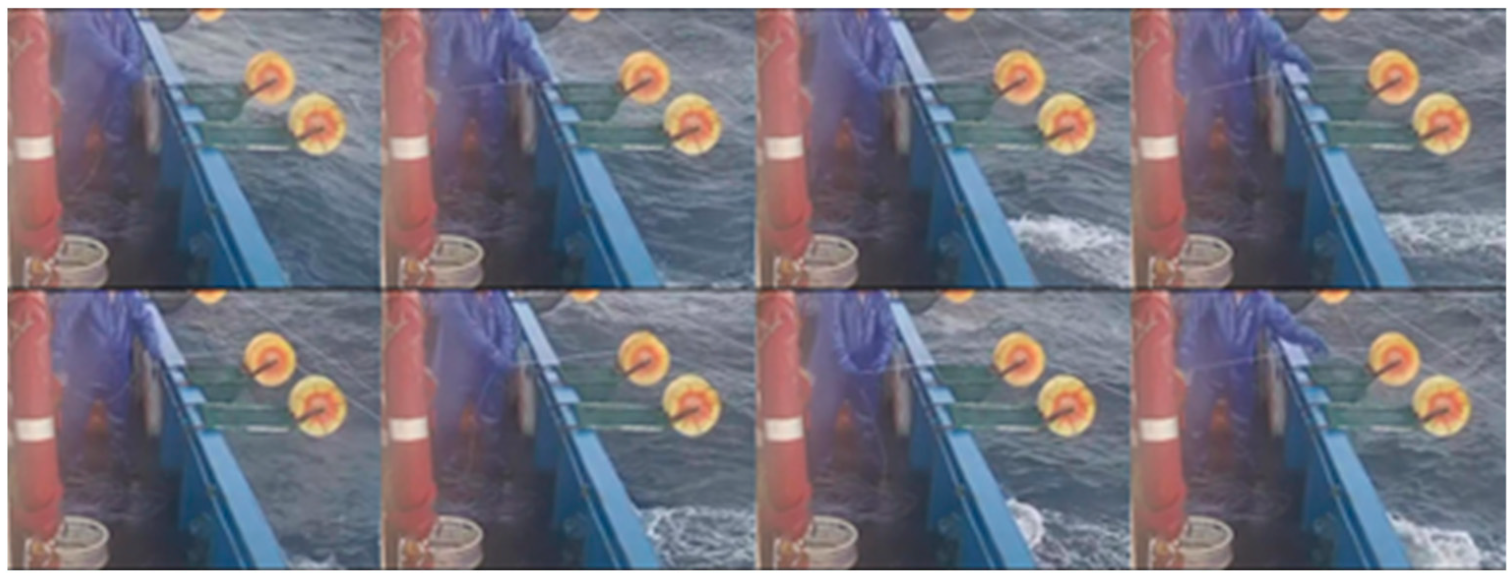
- Add salt-and-pepper noise: Simulate the possible blur of the camera by adding salt-and-pepper noise, allowing the model to learn how to handle blurry images and improve its ability to deal with such situations.
- Vertical flip: Use the ability to vertically flip images to simulate situations that may arise due to incorrect camera orientation.
- Horizontal flip: Simulate different camera and crew positions by horizontally flipping the image, which can simulate fishing behaviors of crew members in different positions on the vessel.
2.3. Network Structure
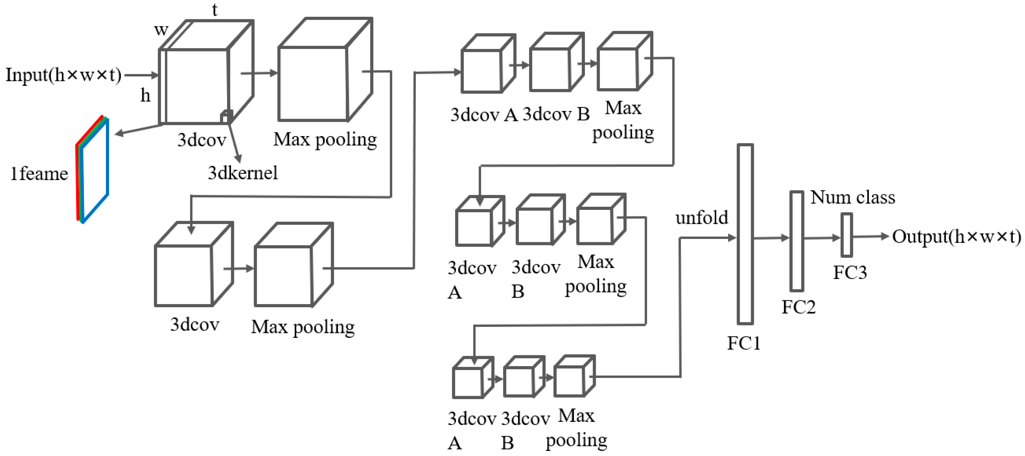
2.3.1. 3DCNN
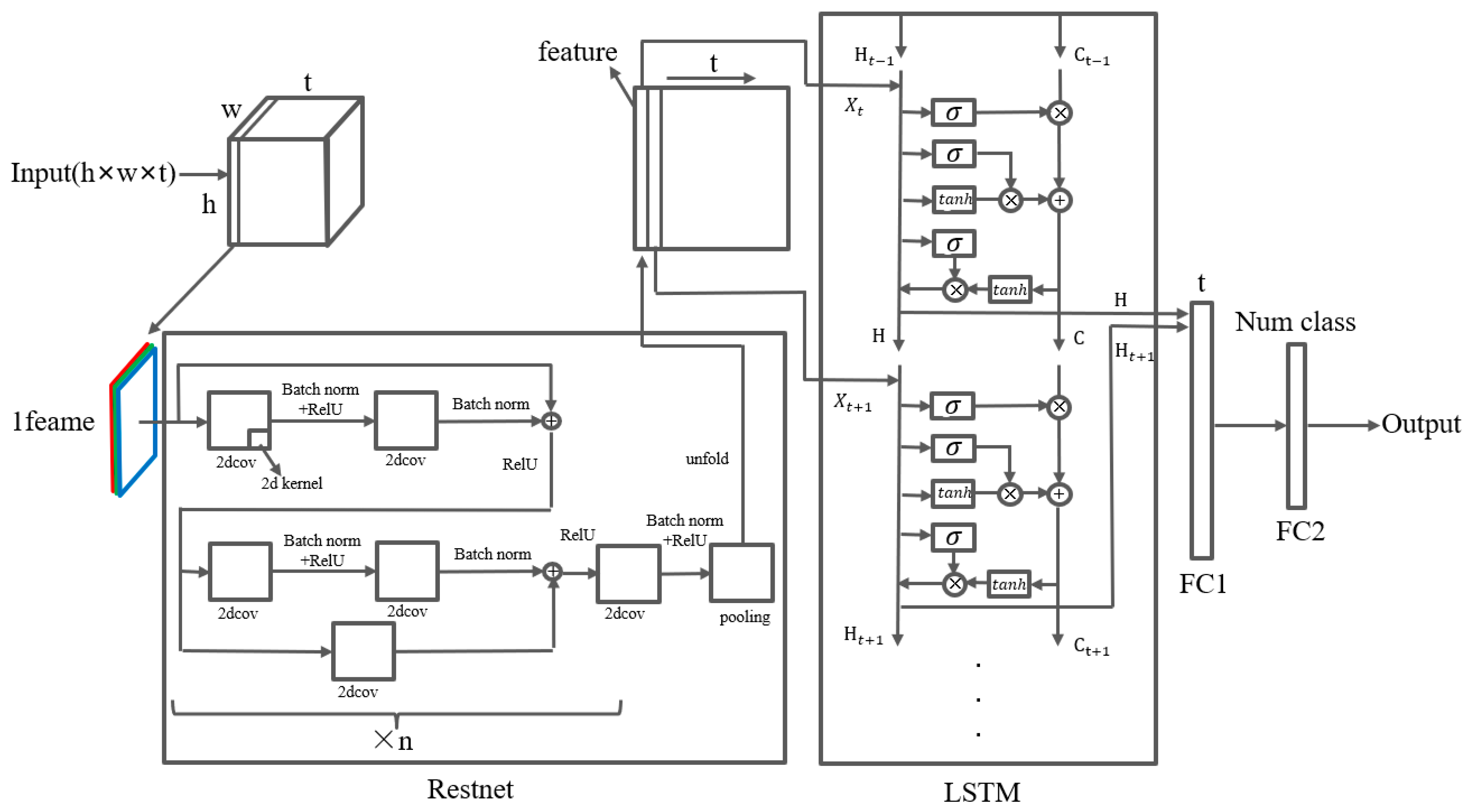
2.3.2. LSTM-ResNet
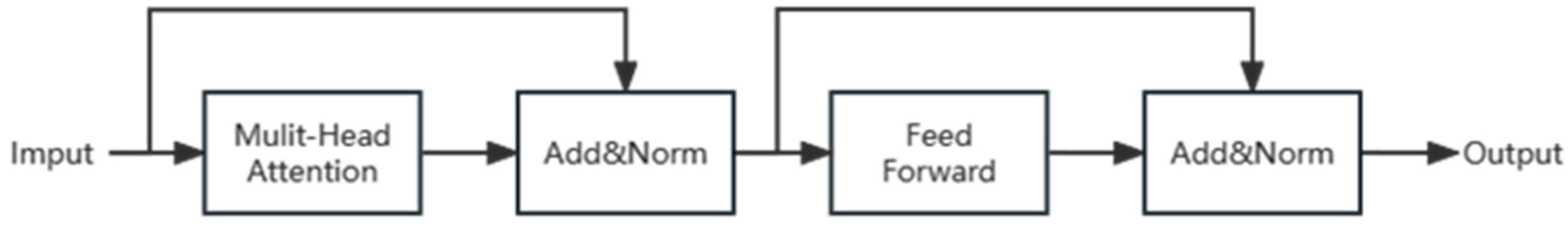
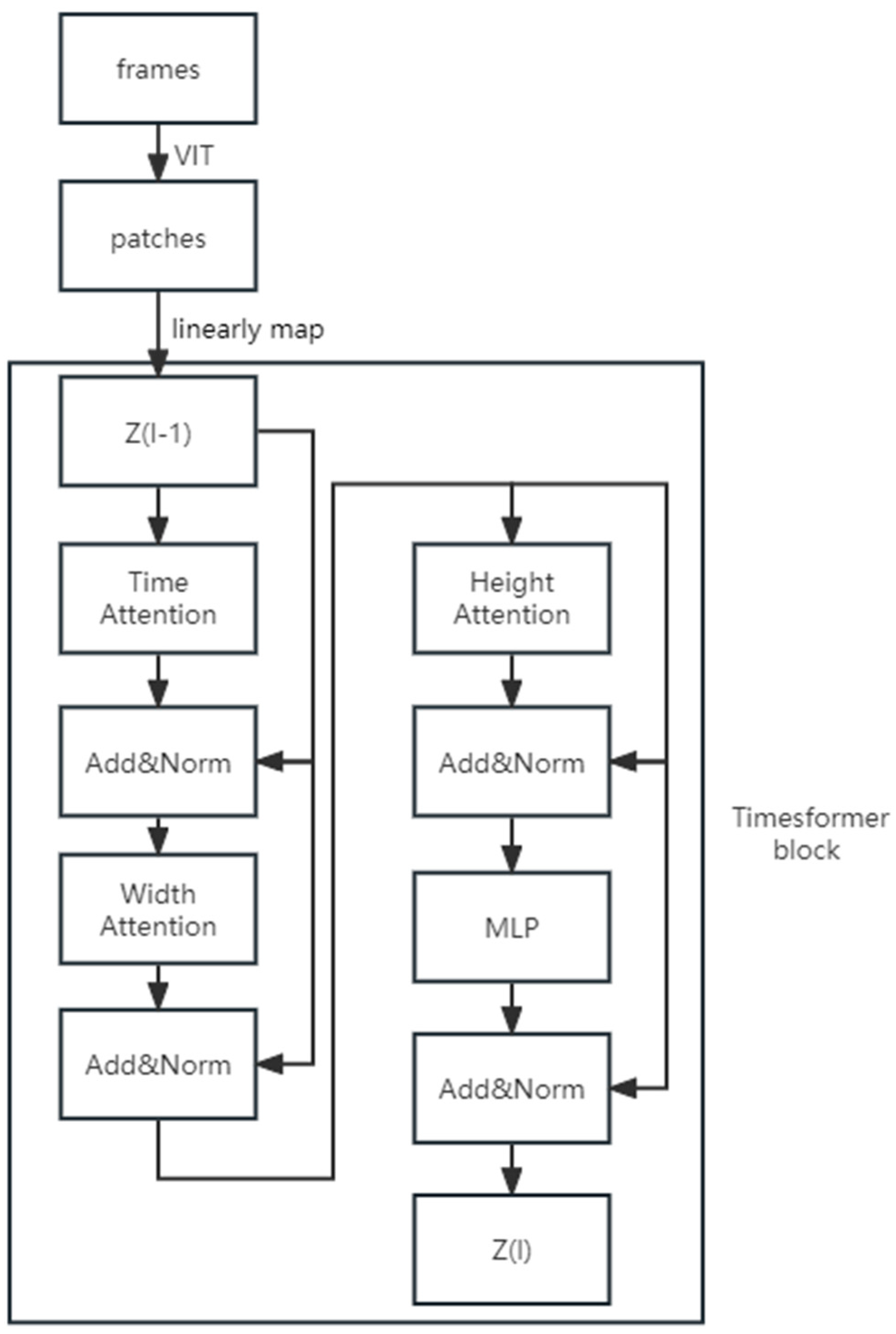
2.3.3. TimeSformer
3. Results
3.1. Evaluation Indicators
- and : represents the ratio of correctly predicted videos () to the total number of videos (). represents the ratio of correctly predicted videos () to the total number of videos (), where any of the top five predicted results are considered correct.
- 2.
- Mean Average Precision (): is a widely used evaluation metric for assessing the performance of a model in multi-class classification tasks. It represents the average precision across all classes. The average precision for each class measures the model’s precision on that class. It is calculated by computing the cross-entropy between the model’s predicted confidence scores and the true labels [25].
- 3.
- : The Score is a measure that represents the weighted average of precision and recall, and it is commonly used to assess the performance of binary classification tasks. Calculation of the Score involves counting the occurrences of true positives, false positives, and false negatives [26].
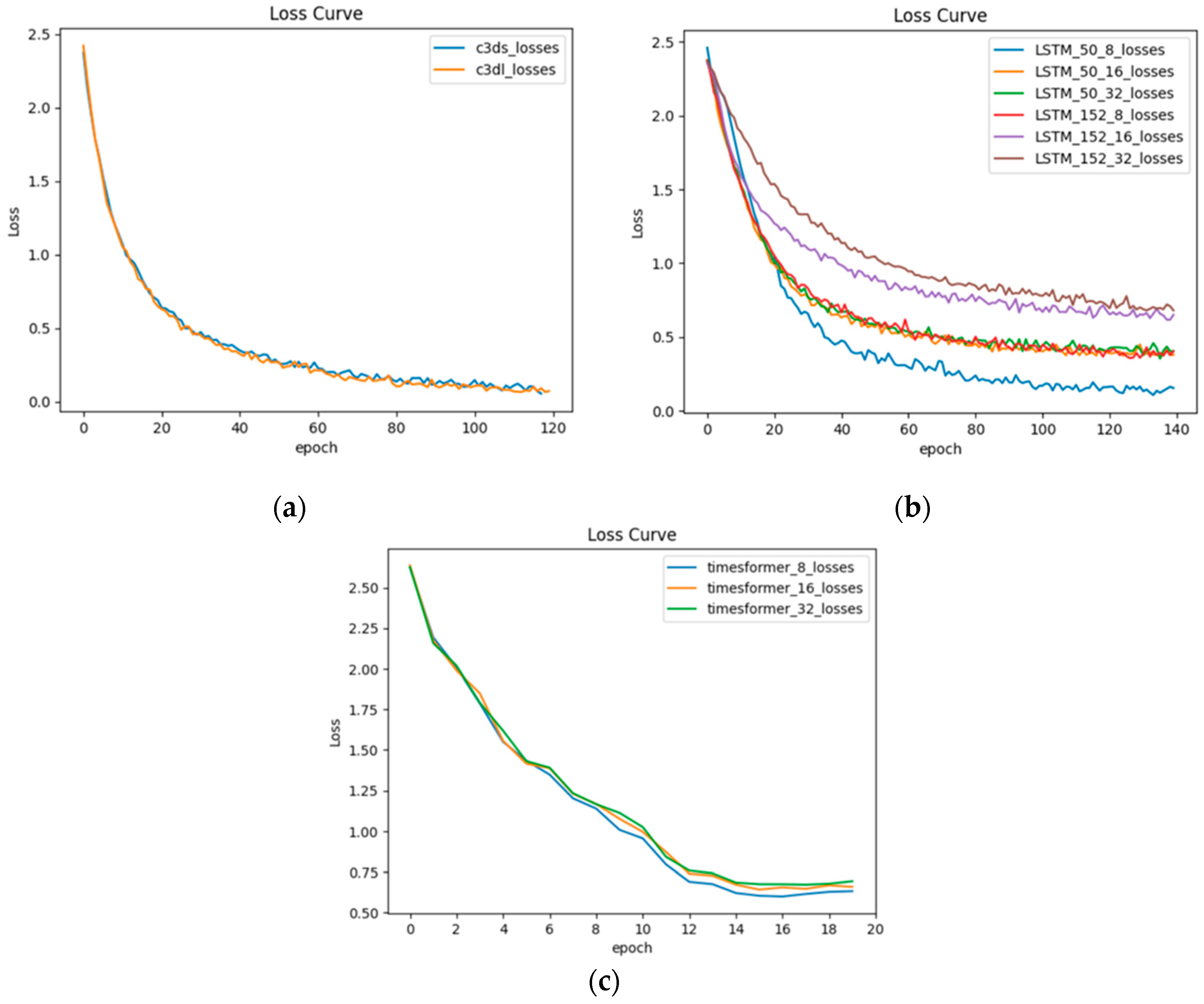
3.2. Experimental Results
4. Discussion
4.1. Data Collection
4.2. Analysis of Model Performance
5. Conclusions
- In this article, the squid fishing dataset was constructed. The LSTM-ResNet-50 model, with NUM_FRAMES set to 8, achieved an accuracy of 88.47%, an score of 0.8881, and an score of 0.8133. In comparison to other parameters, increasing the depth of the ResNet model did not improve the overall performance of the LSTM-ResNet model.
- The 3DCNN-S model outperformed the 3DCNN-L model in terms of the 3DCNN architecture. Nevertheless, the small-scale 3DCNN-S model exhibited a negligible difference compared to the 3DCNN-L model, illustrating its competence in effectively handling the classification task of the squid fishing dataset built in this study.
- In the TimeSformer model, the NUM_FRAMES parameter had minimal impact on the and , but it did influence the and metrics. Nevertheless, the TimeSformer model exhibited poor performance on the squid fishing dataset, which consists of short videos. Nonetheless, it possesses an advantage in training speed compared to the LSTM-ResNet and 3DCNN models. The transformer architecture has significant potential for video-recognition applications.
Author Contributions
Funding
Institutional Review Board Statement
Data Availability Statement
Conflicts of Interest
References
- Chen, C.; Chen, X. Analysis of the research status in the field of offshore fishery based on bibliometrics. Mar. Freshw. Fish. 2020, 175, 108–119. [Google Scholar] [CrossRef]
- Michelin, M.; Elliott, M.; Bucher, M.; Zimring, M.; Sweeney, M. Catalyzing the Growth of Electronic Monitoring in Fisheries: Building Greater Transparency and Accountability at Sea; California Environmental Associates: San Francisco, CA, USA, 2018. [Google Scholar]
- Zhang, J.; Zhang, S.; Fan, W. Research on target detection of Japanese anchovy purse seine based on improved YOLOv5 model. Mar. Fish. 2023, 1–15. [Google Scholar] [CrossRef]
- Ruiz, J.; Batty, A.; Chavance, P.; McElderry, H.; Restrepo, V.; Sharples, P.; Santos, J.; Urtizberea, A. Electronic monitoring trials on in the tropical tuna purse-seine fishery. ICES J. Mar. Sci. 2015, 72, 1201–1213. [Google Scholar] [CrossRef]
- Pei, K.; Zhang, J.; Zhang, S.; Sui, Y.; Zhang, H.; Tang, F.; Yang, S. Spatial distribution of fishing intensity of canvas stow net fishing vessels in the East China Sea and the Yellow Sea. Indian J. Fish. 2023, 70, 1–9. [Google Scholar] [CrossRef]
- Wang, S.; Zhang, S.; Zhu, W.; Sun, Y.; Yang, L.; Sui, J.; Shen, L.; Shen, J. Target detection application of deep learning YOLOV5 network model in electronic monitoring system for tuna longline fishing. J. Dalian Ocean. Univ. 2021, 36, 842–850. [Google Scholar] [CrossRef]
- Zhang, J.; Wang, S.; Zhang, S.; Tang, F.; Fan, W.; Yang, S.; He, R. Research on target detection of engraulis japonicus purse seine based on improved model of YOLOv5. Front. Mar. Sci. 2022, 9, 933735. [Google Scholar] [CrossRef]
- Wang, S.; Zhang, S.; Liu, Y.; Zhang, J.; Sun, Y.; Yang, Y.; Tang, F. Recognition on the working status of Acetes chinensis quota fishing vessels based on a 3D convolutional neural network. Fish. Res. 2022, 248, 106226. [Google Scholar] [CrossRef]
- Ji, S.; Xu, W.; Yang, M.; Yu, K. 3D convolutional neural networks for human action recognition. IEEE Trans. Pattern Anal. Mach. Intell. 2012, 35, 221–231. [Google Scholar] [CrossRef]
- Wu, W.; Sun, Z.; Ouyang, W. Revisiting classifier: Transferring vision-language models for video recognition. Proc. AAAI Conf. Artif. Intell. 2023, 37, 2847–2855. [Google Scholar] [CrossRef]
- Rafiq, M.; Rafiq, G.; Agyeman, R.; Choi, G.S.; Jin, S.I. Scene classification for sports video summarization using transfer learning. Sensors 2020, 20, 1702. [Google Scholar] [CrossRef]
- Varol, G.; Laptev, I.; Schmid, C. Long-term temporal convolutions for action recognition. IEEE Trans. Pattern Anal. Mach. Intell. 2017, 40, 1510–1517. [Google Scholar] [CrossRef]
- Wang, Z.; Li, P.; Chen, B.; Ye, L. Research on sports video classification based on CNN-LSTM encoder-decoder network. J. Jiaxing Univ. 2021, 33, 25–34. [Google Scholar]
- Selva, J.; Johansen, A.S.; Escalera, S.; Nasrollahi, K.; Moeslund, T.B.; Clapés, A. Video Transformers: A Survey. In IEEE Transactions on Pattern Analysis and Machine Intelligence; IEEE: Piscataway, NJ, USA, 2023; pp. 1–10. [Google Scholar]
- Brattoli, B.; Tighe, J.; Zhdanov, F.; Perona, P.; Chalupka, K. Rethinking zero-shot video classification: End-to-end training for realistic applications. In Proceedings of the IEEE/CVF Conference on Computer Vision and Pattern Recognition, Seattle, WA, USA, 13–19 June 2020; pp. 4613–4623. [Google Scholar]
- Bertasius, G.; Wang, H.; Torresani, L. Is space-time attention all you need for video understanding? ICML 2021, 2, 4. [Google Scholar]
- Zhi, H.; Yu, H.; Li, S.; Gao, C.; Wang, Y. A video classification method based on deep metric learning. J. Electron. Inf. Technol. 2018, 40, 2562–2569. [Google Scholar]
- Bo, P.; Tang, J.; Cai, X.; Xie, J.; Zhang, Y.; Wang, Y. High Altitude Video Traffic State Prediction Based on 3DCNN-DNN. J. Transp. Syst. Eng. Inf. Technol. 2020, 20, 39–46. [Google Scholar] [CrossRef]
- Vaswani, A.; Shazeer, N.; Parmar, N.; Uszkoreit, J.; Jones, L.; Gomez, A.N.; Polosukhin, I. Attention is all you need. In Advances in Neural Information Processing Systems; MIT Press: Cambridge, MA, USA, 2017; Volume 30. [Google Scholar]
- Rakhimov, R.; Volkhonskiy, D.; Artemov, A.; Zorin, D.; Burnaev, E. Latent video transformer. In Proceedings of the 16th International Joint Conference on Computer Vision, Imaging and Computer Graphics Theory and Applications, Virtual, 8–10 February 2021; pp. 101–112. [Google Scholar]
- Dosovitskiy, A.; Beyer, L.; Kolesnikov, A.; Weissenborn, D.; Zhai, X.; Unterthiner, T.; Houlsby, N. An image is worth 16x16 words: Transformers for image recognition at scale. arXiv 2010, arXiv:2010.11929. [Google Scholar]
- Kim, D.; Xie, J.; Wang, H.; Qiao, S.; Yu, Q.; Kim, H.S.; Chen, L.C. Tubeformer-deeplab: Video mask transformer. In Proceedings of the IEEE/CVF Conference on Computer Vision and Pattern Recognition, New Orleans, LA, USA, 18–24 June 2022; pp. 13914–13924. [Google Scholar]
- Gabeur, V.; Sun, C.; Alahari, K.; Schmid, C. Multi-modal transformer for video retrieval. In Proceedings of the Computer Vision–ECCV 2020: 16th European Conference, Glasgow, UK, 23–28 August 2020; Part IV 16. Springer International Publishing: Cham, Switzerland, 2020; pp. 214–229. [Google Scholar]
- Girdhar, R.; Carreira, J.; Doersch, C.; Zisserman, A. Video action transformer network. In Proceedings of the IEEE/CVF Conference on Computer Vision and Pattern Recognition, Long Beach, CA, USA, 15–20 June 2019; pp. 244–253. [Google Scholar]
- Panda, R.; Chen CF, R.; Fan, Q.; Sun, X.; Saenko, K.; Oliva, A.; Feris, R. Adamml: Adaptive multi-modal learning for efficient video recognition. In Proceedings of the IEEE/CVF International Conference on Computer Vision, Montreal, BC, Canada, 11–17 October 2021; pp. 7576–7585. [Google Scholar]
- Liao, J.; Wang, S.; Zhang, X.; Liu, G. 3d convolutional neural networks based speaker identification and authentication. In Proceedings of the 2018 25th IEEE International Conference on Image Processing (ICIP), Athens, Greece, 7–10 October 2018; pp. 2042–2046. [Google Scholar]
- Liaojian Country. Research on Speaker Recognition and Verification Technology Based on 3DCNN Lip Reading Features; Shanghai Jiao Tong University: Shanghai, China, 2019. [Google Scholar] [CrossRef]
- Affandi, A.; Sumpeno, S. Clustering spatial temporal distribution of fishing vessel based LON VMS data using K-means. In Proceedings of the IEEE 2020 3rd International Conference on Information and Communications Technology (ICOIACT), Yogyakarta, Indonesia, 24–25 November 2020; pp. 1–6. [Google Scholar]
- Gilman, E.; Castejón VD, R.; Loganimoce, E.; Chaloupka, M. Capability of a pilot fisheries electronic monitoring system to meet scientific and compliance monitoring objectives. Mar. Policy 2020, 113, 103792. [Google Scholar] [CrossRef]
- Ullah, I.; Chen, J.; Su, X.; Esposito, C.; Choi, C. Localization and Detection of Targets in Underwater Wireless Sensor Using Distance and Angle Based Algorithms. IEEE Access 2019, 7, 45693–45704. [Google Scholar] [CrossRef]
- Su, X.; Ullah, I.; Liu, X.; Choi, D. A Review of Underwater Localization Techniques, Algorithms, and Challenges. J. Sens. 2020, 2020, 6403161. [Google Scholar] [CrossRef]
- Teng, J.B.; Kong, W.W.; Tian, Q.X.; Wang, Z.Q.; Li, L. Multi-channel attention mechanism text classification model based on CNN and LSTM. Comput. Eng. Appl. 2021, 57, 154–162. [Google Scholar]
- Wu, Z.; Yao, T.; Fu, Y.; Jiang, Y.G. Deep learning for video classification and captioning. Front. Multimed. Res. 2017, 17, 3–29. [Google Scholar]


| Serial Number | Category | Behavior Description | Category Image |
|---|---|---|---|
| 1 | No crew | There are no crew members at the pulley |  |
| 2 | Idle | The crew is at the pulley but not working |  |
| 3 | Hands collect the line | The crew manually pulls the line through the pulley |  |
| 4 | Hands release the line | The crew releases the fishing line through their hands and the pulley |  |
| 5 | Empty hands release the thread | The line is automatically released with the help of ocean current | 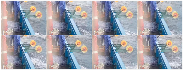 |
| 6 | Use a wire winder to retrieve the cable | The crew uses a wire winder to retrieve the cable | 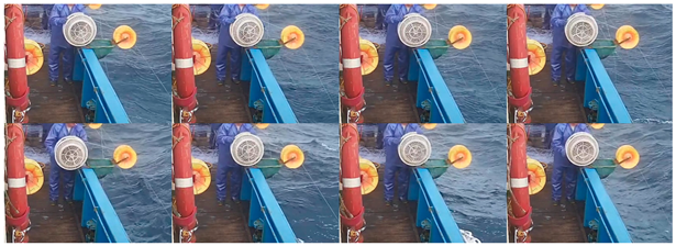 |
| 7 | Use a coil winder to unwind the line | The crew uses a coil winder to unwind the line | 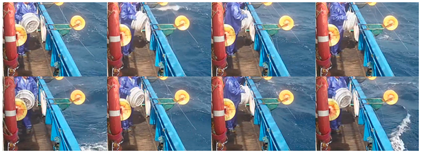 |
| 8 | Untangling the fishing line | The crew unties a knot | 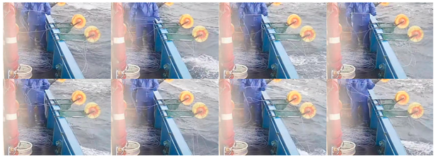 |
| 9 | Handling miscellaneous matters | The crew deals with other tasks at the pulley |  |
| 10 | Pull up the squid | The crew pulls the squid onto the vessel | 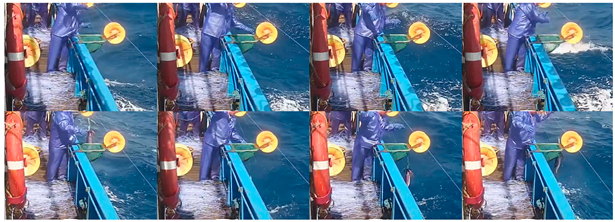 |
| 11 | The squid is placed in the frame | The crew members put the squid into the net | 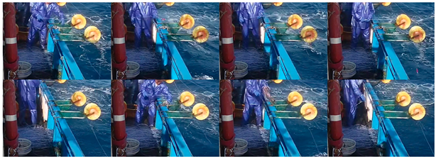 |
| 12 | Receive and release | The crew alternates between pulling and releasing the rope | 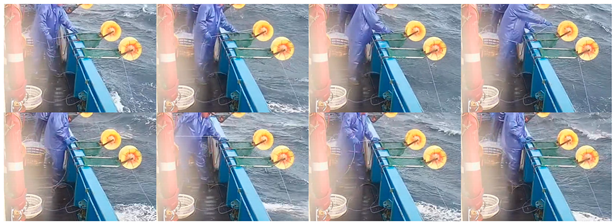 |
| Processed Image | 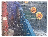 | 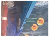 | 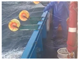 |
| Processing method | Add salt-and-pepper noise | Vertical flipping | Horizontal flipping |
| Video Storage Path. | Category |
|---|---|
| ./path | 1 |
| Model | Evaluation Criteria | |||||
|---|---|---|---|---|---|---|
| 3DCNN | Parameter size | NUM_FRAMES | ||||
| S | 8 | 88.06% | 100.00% | 0.8732 | 0.7835 | |
| L | 87.08% | 100.00% | 0.8622 | 0.7763 | ||
| LSTM | Feature-extraction model | NUM_FRAMES | ||||
| ResNet-50 | 8 | 88.75% | 100.00% | 0.8865 | 0.8037 | |
| 16 | 82.36% | 100.00% | 0.8365 | 0.7290 | ||
| 32 | 75.69% | 98.05% | 0.7323 | 0.5973 | ||
| ResNet-152 | 8 | 79.58% | 98.33% | 0.8037 | 0.6743 | |
| 16 | 69.17% | 96.80% | 0.6854 | 0.5027 | ||
| 32 | 63.47% | 96.25% | 0.6184 | 0.4736 | ||
| TimeSformer-L | NUM_FRAMES | |||||
| 8 | 80.83% | 100% | 0.8632 | 0.7275 | ||
| 16 | 79.72% | 100% | 0.8250 | 0.6630 | ||
| 32 | 78.19% | 100% | 0.8367 | 0.6179 | ||
| Model | ||||
|---|---|---|---|---|
| 3DCNN-S-NUM_FRAMES-8 | 83.75% | 98.33% | 0.7809 | 0.6856 |
| LSTM-ResNet-50-NUM_FRAMES-8 | 84.58% | 98.75% | 0.8137 | 0.7563 |
| TimeSformer-L-NUM_FRAMES-8 | 74.16% | 99.58% | 0.7636 | 0.6453 |
Disclaimer/Publisher’s Note: The statements, opinions and data contained in all publications are solely those of the individual author(s) and contributor(s) and not of MDPI and/or the editor(s). MDPI and/or the editor(s) disclaim responsibility for any injury to people or property resulting from any ideas, methods, instructions or products referred to in the content. |
© 2023 by the authors. Licensee MDPI, Basel, Switzerland. This article is an open access article distributed under the terms and conditions of the Creative Commons Attribution (CC BY) license (https://creativecommons.org/licenses/by/4.0/).
Share and Cite
Song, Y.; Zhang, S.; Tang, F.; Shi, Y.; Wu, Y.; He, J.; Chen, Y.; Li, L. Behavior Recognition of Squid Jigger Based on Deep Learning. Fishes 2023, 8, 502. https://doi.org/10.3390/fishes8100502
Song Y, Zhang S, Tang F, Shi Y, Wu Y, He J, Chen Y, Li L. Behavior Recognition of Squid Jigger Based on Deep Learning. Fishes. 2023; 8(10):502. https://doi.org/10.3390/fishes8100502
Chicago/Turabian StyleSong, Yifan, Shengmao Zhang, Fenghua Tang, Yongchuang Shi, Yumei Wu, Jianwen He, Yunyun Chen, and Lin Li. 2023. "Behavior Recognition of Squid Jigger Based on Deep Learning" Fishes 8, no. 10: 502. https://doi.org/10.3390/fishes8100502
APA StyleSong, Y., Zhang, S., Tang, F., Shi, Y., Wu, Y., He, J., Chen, Y., & Li, L. (2023). Behavior Recognition of Squid Jigger Based on Deep Learning. Fishes, 8(10), 502. https://doi.org/10.3390/fishes8100502