Nonlinearity and Spatial Autocorrelation in Species Distribution Modeling: An Example Based on Weakfish (Cynoscion regalis) in the Mid-Atlantic Bight

Abstract

Nonlinearity and spatial autocorrelation are common features observed in marine fish datasets but are often ignored or not considered simultaneously in modeling. Both features are often present within ecological data obtained across extensive spatial and temporal domains. A case study and a simulation were conducted to evaluate the necessity of considering both characteristics in marine species distribution modeling. We examined seven years of weakfish (Cynoscion regalis) survey catch rates along the Atlantic coast, and five types of statistical models were formulated using a delta model approach because of the high percentage of zero catches in the dataset. The delta spatial generalized additive model (GAM) confirmed the presence of nonlinear relationships with explanatory variables, and results from 3-fold cross-validation indicated that the delta spatial GAM yielded the smallest training and testing errors. Spatial maps of residuals also showed that the delta spatial GAM decreased the spatial autocorrelation in the data. The simulation study found that the spatial GAM over competes other models based on the mean squared error in all scenarios. That indicates that the recommended model not just works well for the NEAMAP survey but also for other cases as in the simulated scenarios.

1. Introduction

Species distributional data, such as biological survey data that often include capture location, time, and animal abundance in number or weight, are frequently used for analyzing the relationship between species distribution and environmental factors. Such analyses can help shape the foundation of species management and conservation procedures by predicting future abundance distributions based on future environmental conditions and spatial management policies. Spatial data analysis was introduced into fisheries during the late 1980s to improve understanding of species distribution and stock assessments for spatially aggregated species [1,2], and efforts have been directed at detecting the spatial distribution patterns of fish stocks [3,4].

Spatial data analysis is complex due to spatial autocorrelation and nonlinearity. Spatial autocorrelation is a phenomenon where samples are not independent from each other at nearby locations [5]. Spatial nonlinearity, which reflects the nonlinear relationship between species density and a suite of predictor variables, has been widely observed for many marine species distributions [6,7]. Multiple factors can cause spatial autocorrelation [8,9,10], such as biological processes (i.e., distance-related dispersal or species interactions), inappropriate modeling of nonlinear relationships between environmental factors and species, or failure to incorporate critical environmental variables that exhibit spatial structure [11]. The second and the third factors are sometimes considered spatial dependency rather than spatial autocorrelation [12].

Generalized linear models (GLMs) and generalized additive models (GAMs) are commonly used to model the relationship between catch rates, which are often defined as the number of fish captured per unit of effort, and environmental, spatial, and temporal factors [13,14]. Effort in fisheries surveys can be measured as tow distance, soak time, or spatial area fished. GLMs assume a linear relationship between the link function of the expected value of response variable and explanatory variables [15,16], while GAMs are an extension of GLMs to deal with nonlinear relationships between the link function of the expected value of the response variable and explanatory variables. However, both GLMs and GAMs assume that catch rate observations are independent across the survey domain, which may not be appropriate for fish species that exhibit spatially aggregated distributions. Similar catch rates can occur because many marine fishes live and occur in close proximity to each other. Thus, spatial autocorrelation can be problematic for species distribution modeling and catch rate standardization when using standard GLMs and GAMs. Alternative methods have been used to deal with spatial autocorrelation in biological survey data [17,18], such as the autoregressive model (simultaneous autoregressive model (SAR) and conditional autoregressive model (CAR)), which incorporates a spatial weight matrix where the neighborhood of each sampling location and weight of each neighbor is included in the standard linear model. Another method is the generalized linear mixed model (GLMM), in which the linear predictors include random effect and within subject error can be spatially autocorrelated [19]. Generalized least square (GLS) adds a weight matrix, which is calculated by some correlation functions, on both sides of the regression and obtain least square estimators [20]. The spatial dependence of a location on neighboring locations is modeled within the variance-covariance matrix [21,22,23].

Survey data of weakfish (Cynoscion regalis) along Atlantic coast was used as dataset in this study. Weakfish are found along the western coast of the Atlantic Ocean from New York to North Carolina where they support recreational and commercial fisheries. Since the early 1980s, weakfish landings have declined steadily and have reached a historic low in recent years. Weakfish exhibit northerly, inshore migrations during spring (April–May), entering estuaries and bays along the eastern U.S. coast to feed and spawn. As water temperatures cool during fall (October-November), fish form aggregations and engage in southerly, offshore movements to overwintering grounds. The most recent weakfish stock assessment concluded the stock was depleted with overfishing not occurring. A key research recommendation from the assessment motivated us to conduct temporal and spatial analyses of fishery-independent survey data [24].

The main goal of this study was to diagnose the necessity of considering nonlinearity and spatial autocorrelation in fish distribution based on the case-study weakfish survey data and through a simulation analysis. During this study we also evaluated the performance of spatial, non-spatial, and nonlinear models in analyzing spatially autocorrelated survey data, and explore the influence of environmental factors on catch rate data for weakfish collected from the nearshore mid-Atlantic Bight from southern New England to Cape Hatteras, North Carolina.

2. Materials and Method

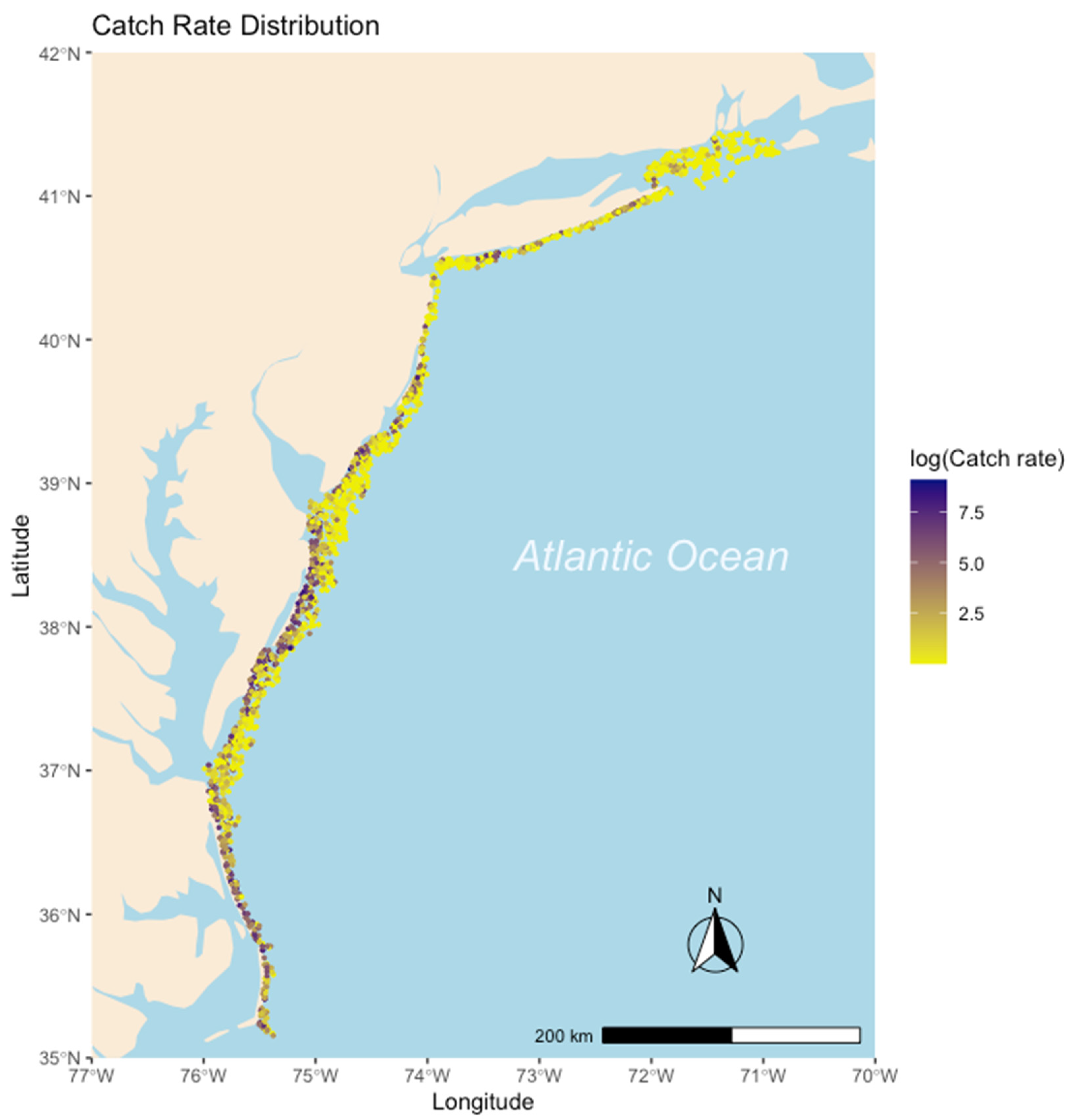
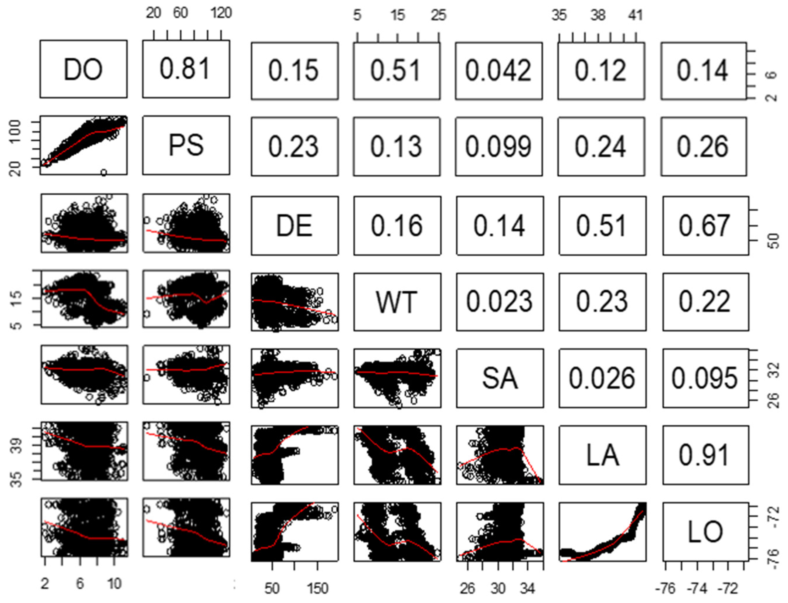
2.1. Weakfish Case Study

The data for weakfish were obtained from a fishery-independent survey, namely the Northeast Area Monitoring and Assessment Program (NEAMAP). We used the NEAMAP survey database from 2007 to 2013, which included 1820 samples. The survey began in fall 2007, and spring and fall cruises have been conducted annually. Locations of sampling sites, which follow a stratified random sampling design, range from 35.16 to 41.44° N, and 70.87 to 75.99° W. The survey area strata were based on longitudinal zones and water depth [25]. The survey area was divided into 7 longitudinal zones from Martha’s Vineyard through New York and 10 latitudinal zones from New Jersey to North Carolina. The boundaries of these zones corresponded roughly with those established by the NEFSC (Northeast Fisheries Science Center’s) Bottom Trawl Survey. For each longitudinal zone, the survey area is also stratified by 4 depth strata: 20–40 ft, 40–60 ft, 60–90 ft, and 90+ ft. The net used by the NEAMAP near shore trawl survey was a three-bridle trawl, the fishing circle of which is 400 meshes of 12 cm, 4 mm braided polyethylene (PE) twine (4800 cm fishing circle). The net codend was made of 12 cm, double 4 mm braided PE with a 2.54 cm knotless nylon liner. The sampling frame consists of 2006 1.5 × 1.5 min cells, with each cell considered to be a sampling unit, and the net is trawled along the bottom for 20 min, at a speed of 2.9–3.3 knots [25]. Eighty samples were removed due to missing values for explanatory variables, reducing the total number of samples to 1740 (Figure 1). Nine explanatory variables were available, including seven continuous variables (depth, water temperature, percentage of oxygen saturation, salinity, dissolved oxygen, latitude, and longitude) and two categorical variables (year and month). Catch rate was calculated as the ratio of biomass collected (kg) and tow distance (m) of the trawl net.

The Spearman correlation among all explanatory variables was examined to detect highly correlated variables. The explanatory variables were selected through a stepwise selection based on Akaike’s Information Criterion (AIC). Interactions between environmental factors were not considered to avoid additional multicollinearity problems and model interpretation difficulties [14,26]. The selected variables from the GLMs were then used in the spatial autoregressive models and autocovariate models because both types are extensions of GLMs.

2.2. Models Considered

Models that considered nonlinearity and spatial autocorrelations were considered beyond the commonly used generalized linear model. We included five types of models: GLM, GAM, spatial GAM, autoregressive model, and auto-covariate regression [27]. These models allowed us to assess the performance of models that accommodating nonlinearity, spatial autocorrelation, or both.

2.2.1. Generalized Linear Model (GLM)

The generalized linear model is among the most commonly used, and the default model structure in the study of species distribution and habitat quality analyses [15]. A GLM is usually written as:

$$g\left(E\left(y\right)\right)={\beta }_0+{\displaystyle \sum }{\beta }_i{x}_i$$

(1)

where $g()$ is the link function, y is the response variable, ${\beta }_0$ is the intercept, ${\beta }_i$ is the fixed-effect coefficient for variable $i$, and $x_i$ is the $i$th explanatory variable [28]. Because the NEAMAP weakfish data contained a large number of zeros (48%) and plots of the nonzero catch rates were positively skewed, delta-lognormal model structures were considered [29]. The delta model is also referred to as a hurdle model, which models zero observations and positive observations fully separately. A delta model contains two components; the first is fitted to estimate the probability of obtaining non-zero captures (Equations (2) and (3)), and the second is fitted to the positive observations (Equation (4)). The final index of relative abundance is obtained by multiplying these two model components [14,29,30,31,32,33,34]. To estimate the probability of nonzero observation, values of 0 (no fish captured) and 1 (at least one fish caught) are regarded as realizations of a Bernoulli random variable with a probability $q$ of positive catch. The parameter$q$ can be estimated by a GLM, which is accomplished through a Bernoulli distribution assumption:

$$\mathrm{Pr}\left(Y=y\right)=\{\begin{array}{c}q\\ 1-q\end{array} \begin{array}{c}y=1\\ otherwise\end{array}$$

(2)

$$\mathit{ln}\left(\frac{q}{1-q}\right)={\alpha }_0+{\displaystyle \sum }{\alpha }_i{x}_i$$

(3)

where $q$ is the probability that at least one weakfish is captured and the $\alpha$’s are the regression coefficients. The model for positive catch, $d$ in this study was assumed to be a normal distribution as follows:

$$\mathit{ln}\left(d\right)={\theta }_0+{\displaystyle \sum }{\theta }_i{x}_i$$

(4)

where the $\theta$’s are the regression coefficients.

2.2.2. Generalized Additive Model (GAM)

A GAM is a nonparametric generalization of a GLM with additive predictors rather than linear predictors [16]. A delta-GAM again makes use of the Bernoulli distribution:

$$\mathit{ln}\left(\frac{q}{1-q}\right)={\alpha }_0+{\displaystyle \sum }{f}_i\left(x_i\right)$$

(5)

where $q$ is the probability of positive observation and $f_i$ is the smoothing function for the explanatory variable $x_i$. A GAM with normal distribution is written as:

$$ln\left(d\right)={\beta }_0+{\displaystyle \sum }{s}_i\left(x_i\right)$$

(6)

where $s_i$ is the smoothing function for the explanatory variable $x_i$.

2.2.3. Spatial GAM

A spatial GAM is an extension of an ordinary GAM by adding an interaction term between longitude and latitude as a smoothing surface. Similarly, a delta spatial GAM makes use of the Bernoulli distribution for the presence or absence of catching:

$$\mathit{ln}\left(\frac{q}{1-q}\right)={\alpha }_0+{\displaystyle \sum }{f}_i\left(x_i\right)+f\left(latitude,longitude\right)$$

(7)

Additionally, spatial GAM with normal distribution is written as:

$$ln\left(d\right)={\beta }_0+{\displaystyle \sum }{s}_i\left(x_i\right)+s\left(latitude,longitude\right)$$

(8)

2.2.4. Autoregressive Models

The delta GLM and delta GAM models are not appropriate for spatially autocorrelated data since observations in the data are not independent. In this situation, autoregressive models could be introduced to the analysis. For the Bernoulli data, an auto-covariate model is applied (see next section for details), while for the positive catch rate observations, autoregressive models are used to account for spatial autocorrelation.

For normally distributed data in linear models, spatial autocorrelation can be incorporated by autoregressive models such as the simultaneous autoregressive model (SAR). SAR models assume that the value of the response variable at location $u$ is not only a function of the explanatory variables, but is also related to the neighboring locations $v$ [23,35,36]. The neighborhood relationship among each location is expressed in an $n\times n$ binary spatial weight matrix ($W$), with elements ($w_{uv}$) representing connections between $u$ and $v$. The spatial weight matrix is specified by identifying the neighborhood structure of each cell. Here, the neighborhood was defined to be 100 km as determined by the semivariogram.

For the positive catch rate data, three different SAR models were compared to explore various hypotheses about the occurrence of spatial autocorrelation [20,35]. The SAR error model assumes that spatial autocorrelation is found only in the error term such that the GLM ($Y=X\beta +\epsilon$) is augmented by the inclusion of a spatial structure term ($\lambda W$) with the spatial error term ($\mu$):

$$Y=X\beta +\lambda W\mu +\epsilon$$

(9)

where $\lambda$ is the spatial autoregression coefficient, $W$ is the spatial weight matrix, $\beta$ is a vector representing the slopes associated with the predictors in the original predictor matrix $X$, and $\epsilon$ is the identically distributed independent error. The SAR lag model assumes the autoregression process only occurs in the response variable (“inherent spatial autocorrelation”), and includes the term ($\rho W$) to account for the spatial autocorrelation in the response variable:

$$Y=\rho WY+X\beta +\epsilon$$

(10)

where $\rho$ is the autoregression coefficient, and the remaining terms are as above. The SAR mixed model assumes spatial autocorrelation in both the response and predictor variables. In this case, another term ($WX\gamma$) is introduced in the model, which represents the regression coefficients ($\gamma$) of spatial lagged explanatory variables ($WX$):

$$Y=\rho WY+X\beta +WX\gamma +\epsilon$$

(11)

2.2.5. Auto-Covariate Regression

Applications of SAR models to binary data have been limited [26,37]. However, auto-covariate regression is applicable in this situation, which is an extension of the Bernoulli GLM by adding a distance-weighted function of neighboring responses [38]. The additional parameter is referred to as an auto-covariate, which is, in this case, applied to capture the spatial autocorrelation within Equations (3) and (5) of the delta-GLM and delta-GAM models, respectively.

An auto-covariate regression is written as,

$$\mathit{ln}\left(\frac{q}{1-q}\right)=X\theta +\rho A$$

(12)

where $q$ is the probability of positive observation, $\theta$ is a vector of fixed-effect coefficients, X is a matrix of explanatory variables, $\rho$ is the covariate of A such that

$$A=\frac{{{\displaystyle \sum }}_{jϵk}{w}_{ij}{y}_j}{{{\displaystyle \sum }}_{jϵk}{w}_{ij}} \left(\mathrm{the}\mathrm{weighted}\mathrm{average}\right)$$

(13)

where $y_j$ is the response value at site $j$ among $i$’s set of $k_i$ neighbors and $w_{ij}$ is the weight given to site $j$’s influence over site $i$ [39]. The auto-covariate regression was used for the presence-absence data and combined with SAR models to form delta SAR models.

2.2.6. Software

All the analyses were conducted in R version 4.0.2 [40]. Parameters of the GLMs and auto covariate model were estimated using the “glm” function. Parameters of the GAMs were estimated using “gam” function in the “mgcv” package [41]. Parameters of the SAR error model were estimated using the “errorsarlm” function, and parameters of the SAR lag model and SAR mixed model were estimated using the “lagsarlm” function from the “spatialreg” package [42].

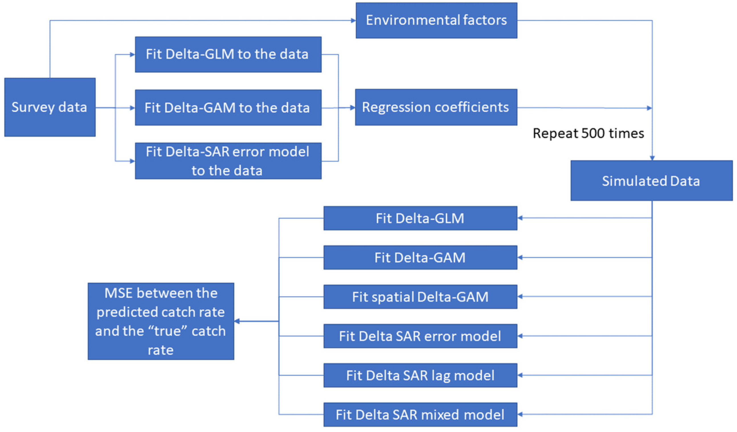
2.3. Simulation

Three simulation scenarios were conducted, respectively with delta GLM, delta GAM, spatial delta GAM, and delta autoregressive models to compare their performances across the survey area under different scenarios (Figure 2). In the first scenario, a delta GLM is fitted to the real survey data to estimate the coefficient of each explanatory variable and the regression residuals. The “true” abundance at each survey point was simulated by applying the estimated coefficient from the delta GLM to the explanatory variables and calculating the response variable by introducing the variance from the regression residuals. Then, delta GAM, spatial delta GAM, and delta spatial models were fitted to the simulated data, respectively, and a standardized catch rate was be obtained. Lastly, the mean squared error between the predicted catch rate and the “true” catch rate was calculated. In the second and third scenarios, we used the same procedure except the simulated catch rates were from delta GAM and delta SAR error models, respectively. Five hundred simulations were conducted for each scenario.

2.4. Model Evaluation

Three model selection approaches were considered to select the most appropriate model: (1) AIC [43], (2) spatial distribution maps of the spatial pattern of the distribution of residuals and correlogram plots, and (3) cross-validation. AIC provides insight about model goodness-of-fit and complexity, the correlogram plots are indicative of Moran’s coefficient on distance classes, and cross-validation can assess the performance of model prediction.

2.4.1. Akaike’s Information Criterion (AIC)

The AIC function is expressed as:

$$\mathrm{AIC}=-2\ln \left(L\right)+2p$$

(14)

where p is the number of parameters in the model and L is the maximized value of the likelihood function for the model. AIC is particularly useful when dealing with the trade-off between model complexity and goodness-of-fit, and the model with minimum AIC value is preferred.

2.4.2. Cross-Validation

Multi-fold cross-validation was used to assess model fit (training error) and prediction accuracy (test error) [16,26]. To conduct k-fold cross-validation, the full dataset was randomly divided into k sub-datasets with equal sizes. Each sub-dataset was then used as a test dataset to predict, while the remaining k-1 sub-datasets were considered as training data for model fitting. Training and test error was computed as:

$$\mathrm{Training}(\mathrm{Test})\mathrm{error}=\frac{1}{N}{{\displaystyle \sum }}_{i=1}^N{(y_i-{\widehat{y}}_i)}^2$$

(15)

where N is the number of observations, $y_i$ is the ith observation, and ${\widehat{y}}_i$ is the estimated value. Three-fold cross-validations were performed for the delta models for 500 iterations, and the model that produced lower training and testing errors was preferred.

3. Results

Correlation coefficients among explanatory variables were high between latitude and longitude (0.91), dissolved oxygen and percentage of oxygen saturation (0.81), and water temperature and month (0.89) (Figure 3). Take water temperature and month for example: both GLM and GAM models that included month and water temperature yielded the smallest AICs (

Table 1. AIC comparison of the three variable selection scenarios for each six model types fitted to NEAMAP weakfish survey data. Scenario 1: month but no water temperature; Scenario 2: water temperature but no month; Scenario 3: both water temperature and month.

	Scenario
	1	2	3
Positive catch model a
GLM	3985	4002	3983
GAM	3925	3886	3883
Spatial GAM	3886	3845	3843
SAR error model	3965	3976	3961
SAR lag model	3975	3989	3972
SAR mixed model	3962	3977	3957
Presence-absence model b
GLM	1741	1785	1717
GAM	1651	1602	1554
Spatial GAM	1487	1445	1408
Auto covariate model	1723	1750	1687

Note: ^a The sub-model in the delta model to estimate the catch rates when only positive values of the response variable were analyzed. ^b The sub-model in the delta model to estimate the probability of obtaining non-zero captures.

). Thus, water temperature and month are kept in all the models. Similarly, variables longitude and percentage of oxygen saturation were eliminated before a stepwise selection for all models. A stepwise procedure was applied to the remaining variables included in the delta models and spatial models, and variables with significant effects (p-values < 0.05) were retained. Thus, the variables kept in all ten models were identical: year, month, water temperature, depth, salinity, and latitude.

Among the candidate model types, the spatial GAM provided the smallest AIC for the positive catch rate data, followed by the GAM (3883, Table 1). The spatial GAM model also produces the smallest AIC value for estimating the probability of positive catches, followed by the GAM (1554).

Residuals of all six candidate model types yielded significant Moran’s I statistics (

Table 2. Moran’s I value of residuals of the six delta models fitted to NEAMAP weakfish survey data.

Model	Delta GLM	Delta GAM	Delta Spatial GAM	Delta SAR Error Model	Delta SAR Lag Model	Delta SAR Mixed Model
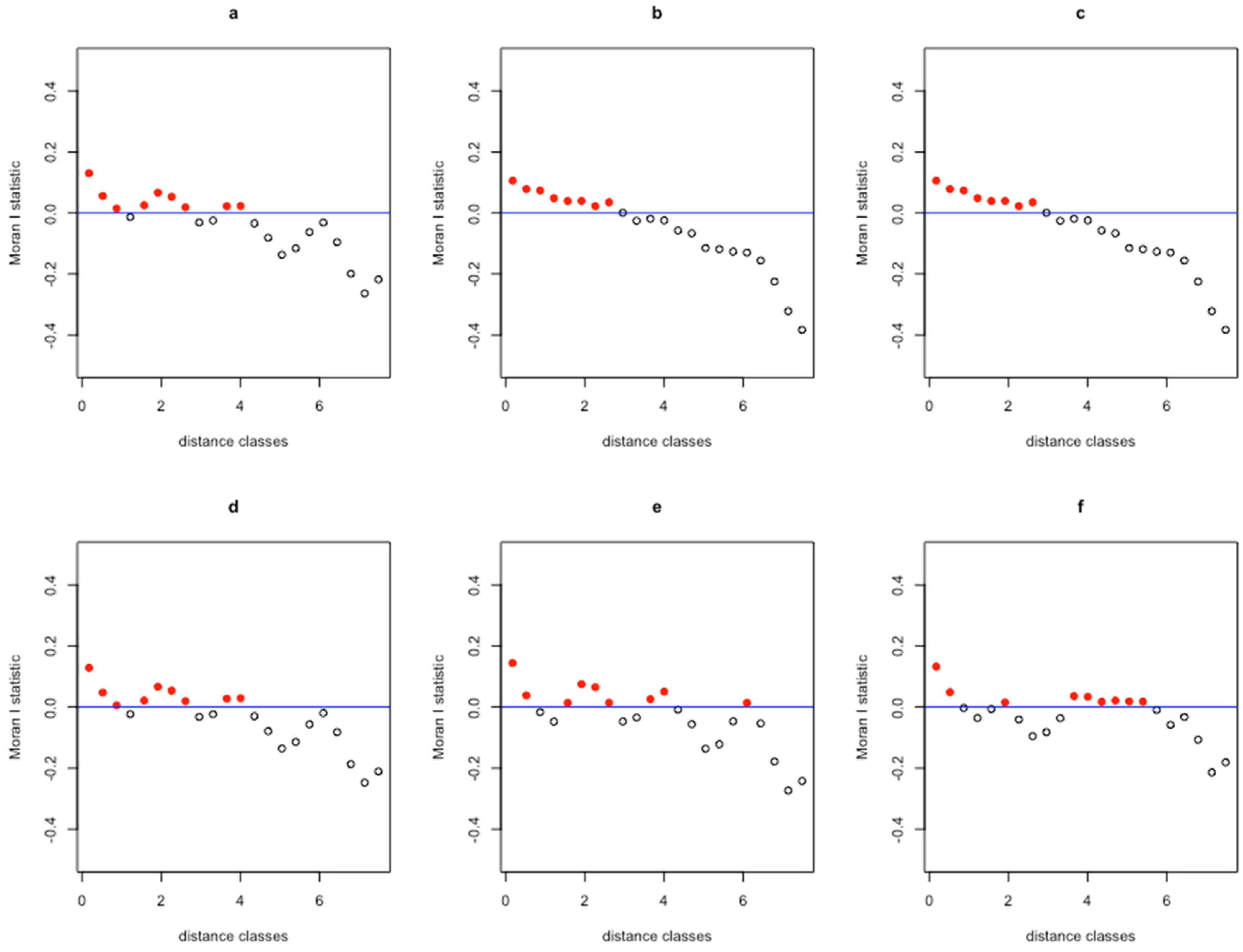
Moran’s I	0.21	0.18	0.20	0.21	0.22	0.55
p-value	<0.001	<0.001	<0.001	<0.001	<0.001	<0.001

). The spatial correlogram plots showed that the presence of spatial autocorrelation in the residuals was evenly distributed for the fitted spatial autocorrelation models (Figure 4). The different spatial autocorrelation models tended to capture spatial autocorrelation at different scales. For example, the delta spatial GAM and delta GAM models managed to consistently decrease spatial autocorrelation in the residuals, while the delta SAR mixed model could not eliminate it.

Maps of residuals from the six delta models indicated that the delta spatial GAM was less autocorrelated when compared to the other models (Figure 5, Figure A1, Figure A2, Figure A3, Figure A4, Figure A5 and Figure A6 for the larger view). The primary reasons supporting this conclusion are the lack of dark points of residuals and the general similarity in color. The residuals maps of the delta SAR lag model and delta SAR mixed model exhibit darker red and darker blue points, suggesting that these two models cannot adequately accommodate the autocorrelation in the data.

Results of the 3-fold cross-validation indicated that the delta spatial GAM model provided the smallest training error and testing error on average, followed by the delta GAM and delta SAR error models (

Table 3. Training and test errors from 3-fold cross-validation for six delta models fitted to NEAMAP weakfish survey data after 500 iterations.

Model	Delta GLM	Delta GAM	Delta Spatial GAM	Delta SAR Error Model	Delta SAR Lag Model	Delta SAR Mixed Model
Training error	5.46	5.03	4.78	5.40	6.74	8.03
Testing error	5.55	5.21	5.01	5.50	6.26	6.36

). This result, in combination with the generally favorable delta spatial GAM residual maps, supports that the spatial GAM best performed in fitting weakfish spatial distribution in the mid-Atlantic Bight.

In the simulation, the delta spatial GAM achieved the smallest mean squared error between predicted and “true” abundance when compared to other candidate models, and the delta GAM ranked second in all three scenarios, regardless of the “true” models (

Table 4. Simulation error for six delta models fitted to NEAMAP weakfish survey data after 500 iterations. The “true” models are the models used for data generation.

“True” Model	Delta GLM	Delta GAM	Delta Spatial GAM	Delta SAR Error Model	Delta SAR Lag Model	Delta SAR Mixed Model
GLM	85.75	85.58	85.51	85.88	85.93	86.00
GAM	191.14	190.97	190.94	191.31	191.43	191.91
SAR error model	99.18	99.07	99.03	99.34	99.41	99.56

). The other spatial models did not perform as well as the non-spatial models and the delta SAR mixed model performed the worst in all three scenarios.

4. Discussion

Our analyses provide evidence that the delta spatial GAM performs well when fitted to data with appreciable spatial autocorrelation and a high percentage of zeroes. Failing to account for spatial autocorrelation among samples may cause imprecision and inaccuracy in parameter estimation, inferences regarding the importance of explanatory variables, and model predictions [37]. However, with spatial models, over-fitting may decrease the prediction ability, and over-fitting usually occurs when a model is excessively complex. The inclusion of a spatial weight matrix based on neighboring samples does increase the complexity of spatial autoregressive models. Although the SAR model performed well in this study, its application does present a tradeoff between formally modeling spatial autocorrelation and a tradeoff between formally modeling spatial autocorrelation on one hand, and concerns about bias and precision on the other hand. Compared to the GLM models, all the spatial autoregressive models yielded smaller AIC values for both the positive catch rate data and the probability of non-zero catches. However, from 3-fold cross-validation, the training and testing errors from the delta SAR lag model and delta SAR mixed model are larger than those from delta GLM, indicating that over-fitting might be a problem when a delta SAR lag model or delta SAR mixed model is used.

Accommodating zero observations in spatial and non-spatial models is a well-documented challenge [44], particularly for datasets that exhibit positively skewed distributions (e.g., lognormal). Delta models along with zero-inflated and hurdle models, are commonly used to analyze fish survey data when a large fraction of zero observations is present. In general, delta GLM and delta (or delta spatial) GAM models are relatively easy to construct, but for spatial auto-regressive models, which can only be fitted to normally distributed data not containing excessive zero observations, we were forced to combine SAR and auto covariate regression models. In this application, the auto covariate regression model played the role of the Bernoulli models in delta GLM and delta GAM.

Variable selection is difficult when explanatory variables are collinear. SAR models are extensions of GLMs such that the variable selection strategies for SAR models are the same as those for GLMs. The explanatory variables month and water temperature were highly correlated and including both within the GLMs implied model over-fitting. However, variable selection strategies for GAMs can be relaxed when compared to those for GLMs, because the smoothing functions can often turn explanatory variables into non-parametric forms, thus making two linearly dependent variables independent [45]. In this study, the variables month and water temperature could both be included in the GAMs, which likely contributed to those models providing better fits to the weakfish catch rate data than the GLMs.

All types of statistical models have their own strengths and weakness, and each can provide distinctive clarity on the importance of specific explanatory variables. One of the favorable properties of the delta spatial GAM and delta GAM is that they can yield stable and accurate estimation and prediction without incurring additional model complexity necessary to accommodate spatial autocorrelation [14]. While this result holds for weakfish catch rate data collected in the mid-Atlantic Bight by the NEAMAP survey, generalizing it to the various types of spatially autocorrelated data commonly collected in the natural sciences warrants further investigation. Another advantage of GAMs is their ability to accommodate nonlinear relationships among response and explanatory variables, which were evident in our results (Figure 6 and Figure 7) and have been shown for other fisheries data [25]. The dramatic drop of AIC values in GAMs compared to GLMs and other spatial models also indicated the superiority of GAMs in dealing with non-linearity in the data (Table 1).

In this analysis, Moran’s I values of residuals from the six candidate models were all significant, indicating spatial autocorrelation was still present (Figure 4). This problem might be due to insufficient explanatory variables, as only four environmental explanatory variables (water temperature, salinity, depth, and latitude) were considered in the models, and two of them were environmental factors (i.e., salinity and depth). All available explanatory variables measured synoptically with sampling were explored. However, it remains possible that other key variables significantly influence the abundance and spatial distribution of weakfish in the mid-Atlantic. Further, broader scale temporal and spatial variables (e.g., climate, environmental, anthropogenic) not examined in this study could be structuring weakfish in the mid-Atlantic, and analyses of these represent critical next steps.

In general, the delta spatial GAM performs well when fitted to the NEAMAP catch rate data for weakfish. We can also see that delta GAM is preferred for estimation and prediction but still has difficulty fully explaining spatial autocorrelation. While the SAR error model comparatively explains the spatial autocorrelation better, it cannot accommodate the nonlinearities among catch rate and explanatory variables revealed by the delta GAM. Delta spatial GAM combines the advantages of delta GAM and delta SAR error model: explaining the spatial autocorrelation as well as accommodating the nonlinearity. This conclusion may not hold for all fish species, and the model result may not remain the same for other datasets. However, this method could be a good option when dealing with nonlinearity and spatial autocorrelation especially when there are large amounts of zero observations. Future fieldwork for the NEAMAP survey could focus on collecting more related variables measured with sampling.

References

- Conan, G. Assessment of shellfish stocks by geostatistical techniques. ICES CM 1985, 1985, 372. [Google Scholar]
- Freire, J.; González-Gurriarán, E.; Fernández, L. Geostatistical analysis of spatial distribution of Liocarcinus depurator, Macropipus tuberculatus and Polybius henslowii (Crustacea: Brachyura) over the Galician continental shelf (NW Spain). Mar. Biol. 1993, 115, 453–461. [Google Scholar]
- Vignaux, M. Analysis of spatial structure in fish distribution using commercial catch and effort data from the New Zealand hoki fishery. Can. J. Fish. Aquat. Sci. 1996, 53, 963–973. [Google Scholar] [CrossRef]
- Walter, J.F., III; Christman, M.C.; Hoenig, J.M.; Mann, R. Combining data from multiple years or areas to improve variogram estimation. Environ. Off. J. Int. Environ. Soc. 2007, 18, 583–598. [Google Scholar] [CrossRef]
- Tobler, W.R. A Computer Movie Simulating Urban Growth in the Detroit Region. Econ. Geogr. 1970, 46, 234–240. [Google Scholar] [CrossRef]
- Yu, H.; Jiao, Y.; Winter, A. Catch-Rate Standardization for Yellow Perch in Lake Erie: A Comparison of the Spatial Generalized Linear Model and the Generalized Additive Model. Trans. Am. Fish. Soc. 2011, 140, 905–918. [Google Scholar] [CrossRef]
- Drexler, M.; Ainsworth, C.H. Generalized Additive Models Used to Predict Species Abundance in the Gulf of Mexico: An Ecosystem Modeling Tool. PLoS ONE 2013, 8, e64458. [Google Scholar] [CrossRef]
- Legendre, P. Spatial autocorrelation: Trouble or new paradigm? Ecology 1993, 74, 1659–1673. [Google Scholar] [CrossRef]
- Legendre, P.; Fortin, M.J. Spatial pattern and ecological analysis. Vegetatio 1989, 80, 107–138. [Google Scholar] [CrossRef]
- Legendre, P.; Legendre, L. Numerical Ecology; Elsevier: Amsterdam, The Netherlands, 2012. [Google Scholar]
- Besag, J. Spatial interaction and the statistical analysis of lattice systems. J. R. Stat. Soc. Ser. B Methodol. 1974, 36, 192–225. [Google Scholar] [CrossRef]
- Legendre, P.; Dale, M.R.; Fortin, M.J.; Gurevitch, J.; Hohn, M.; Myers, D. The consequences of spatial structure for the design and analysis of ecological field surveys. Ecography 2002, 25, 601–615. [Google Scholar] [CrossRef]
- McCullagh, P.; Nelder, J. Binary Data. In Generalized Linear Models; Springer: Berlin/Heidelberg, Germany, 1989; pp. 98–148. [Google Scholar]
- Maunder, M.N.; Punt, A.E. Standardizing catch and effort data: A review of recent approaches. Fish. Res. 2004, 70, 141–159. [Google Scholar] [CrossRef]
- Nelder, J.A.; Wedderburn, R.W. Generalized linear models. J. R. Stat. Soc. Ser. A Gen. 1972, 135, 370–384. [Google Scholar] [CrossRef]
- Hastie, T.; Tibshirani, R.; Friedman, J.H.; Friedman, J.H. The Elements of Statistical Learning: Data Mining, Inference, and Prediction; Springer: Berlin/Heidelberg, Germany, 2009; Volume 2. [Google Scholar]
- Zimmermann, N.E.; Edwards, T.C., Jr.; Graham, C.H.; Pearman, P.B.; Svenning, J.C. New trends in species distribution modelling. Ecography 2010, 33, 985–989. [Google Scholar] [CrossRef]
- Dormann, C.F.; McPherson, J.M.; Araújo, M.B.; Bivand, R.; Bolliger, J.; Carl, G.; Davies, R.G.; Hirzel, A.; Jetz, W.; Kissling, W.D.; et al. Methods to account for spatial autocorrelation in the analysis of species distributional data: A review. Ecography 2007, 30, 609–628. [Google Scholar] [CrossRef]
- Pinheiro, J.; Bates, D. Mixed-Effects Models in S and S-PLUS; Springer Science & Business Media: Berlin/Heidelberg, Germany, 2006. [Google Scholar]
- Cliff, A.D.; Ord, J.K. Spatial Processes: Models & Applications; Taylor & Francis: Abingdon-on-Thames, UK, 1981. [Google Scholar]
- Anselin, L. Spatial Econometrics: Methods and Models; Springer Science & Business Media: Berlin/Heidelberg, Germany, 1988; Volume 4. [Google Scholar]
- Anselin, L.; Bera, A.K. Spatial dependence in linear regression models with an introduction to spatial econometrics. Stat. Textb. Monogr. 1998, 155, 237–290. [Google Scholar]
- Cressie, N. Statistics for Spatial Data; John Wiley & Sons: Hoboken, NJ, USA, 1993. [Google Scholar]
- NEFSC. 48th Northeast Regional Stock Assessment Workshop (48th SAW) Assessment Summary Report, Part C: Weakfish Assessment Summary for 2009; National Marine Fisheries Service: Silver Spring, MD, USA, 2009. [Google Scholar]
- Bonzek, C.; Gartland, J.; Johnson, R.; Lange Jr, J. NEAMAP Near Shore Trawl Survey: Peer Review Documentation; A report to the Atlantic States Marine Fisheries Commission by the Virginia Institute of Marine Science; Virginia Institute of Marine Science: Gloucester Point, VA, USA, 2008. [Google Scholar]
- Damalas, D.; Megalofonou, P.; Apostolopoulou, M. Environmental, spatial, temporal and operational effects on swordfish (Xiphias gladius) catch rates of eastern Mediterranean Sea longline fisheries. Fish. Res. 2007, 84, 233–246. [Google Scholar] [CrossRef]
- Wu, H.; Huffer, F. Modelling the distribution of plant species using the autologistic regression model. Environ. Ecol. Stat. 1997, 4, 31–48. [Google Scholar] [CrossRef]
- Montgomery, D.C.; Peck, E.A.; Vining, G.G. Introduction to Linear Regression Analysis; John Wiley & Sons: Hoboken, NJ, USA, 2006. [Google Scholar]
- Ortiz, M.; Legault, C.M.; Ehrhardt, N.M. An alternative method for estimating bycatch from the US shrimp trawl fishery in the Gulf of Mexico, 1972–1995. Fish. Bull. 2000, 98, 583. [Google Scholar]
- Lo, N.C.-H.; Jacobson, L.D.; Squire, J.L. Indices of Relative Abundance from Fish Spotter Data based on Delta-Lognornial Models. Can. J. Fish. Aquat. Sci. 1992, 49, 2515–2526. [Google Scholar] [CrossRef]
- Pennington, M. Estimating the mean and variance from highly skewed marine data. Fish. Bull. 1996, 94, 498–505. [Google Scholar]
- Stefansson, G. Analysis of groundfish survey abundance data: Combining the GLM and delta approaches. ICES J. Mar. Sci. 1996, 53, 577–588. [Google Scholar] [CrossRef]
- Ye, Y.; Al-Husaini, M.; Al-Baz, A. Use of generalized linear models to analyze catch rates having zero values: The Kuwait driftnet fishery. Fish. Res. 2001, 53, 151–168. [Google Scholar] [CrossRef]
- Murray, K.T. Magnitude and distribution of sea turtle bycatch in the sea scallop (Placopecten magellanicus) dredge fishery in two areas of the northwestern Atlantic Ocean, 2001–2002. Fish. Bull. 2004, 102, 671–681. [Google Scholar]
- Lichstein, J.W.; Simons, T.R.; Shriner, S.A.; Franzreb, K.E. Spatial autocorrelation and autoregressive models in ecology. Ecological monographs 2002, 72, 445–463. [Google Scholar] [CrossRef]
- Haining, R.P.; Haining, R. Spatial Data Analysis: Theory and Practice; Cambridge University Press: Cambridge, UK, 2003. [Google Scholar]
- Dormann, C.F. Effects of incorporating spatial autocorrelation into the analysis of species distribution data. Glob. Ecol. Biogeogr. 2007, 16, 129–138. [Google Scholar] [CrossRef]
- Knapp, R.A.; Matthews, K.R.; Preisler, H.K.; Jellison, R. Developing probabilistic models to predict amphibian site occupancy in a patchy landscape. Ecol. Appl. 2003, 13, 1069–1082. [Google Scholar] [CrossRef]
- Gumpertz, M.L.; Graham, J.M.; Ristaino, J.B. Autologistic Model of Spatial Pattern of Phytophthora Epidemic in Bell Pepper: Effects of Soil Variables on Disease Presence. J. Agric. Biol. Environ. Stat. 1997, 2, 131. [Google Scholar] [CrossRef]
- R Core Team. R: A Language and Environment for Statistical Computing; R Foundation for Statistical Computing: Vienna, Austria, 2021. [Google Scholar]
- Wood, S.N. Fast stable restricted maximum likelihood and marginal likelihood estimation of semiparametric generalized linear models. J. R. Stat. Soc. Ser. B 2010, 73, 3–36. [Google Scholar] [CrossRef]
- Bivand, R.; Millo, G.; Piras, G. A Review of Software for Spatial Econometrics in R. Mathematics 2021, 9, 1276. [Google Scholar] [CrossRef]
- Akaike, H. Information theory and an extension of the maximum likelihood principle. In Selected Papers of Hirotugu Akaike; Parzen, E., Tanabe, K., Kitagawa, G., Eds.; Springer: New York, NY, USA, 1998; pp. 199–213. [Google Scholar]
- Li, Y.; Jiao, Y.; He, Q. Decreasing uncertainty in catch rate analyses using Delta-AdaBoost: An alternative approach in catch and bycatch analyses with high percentage of zeros. Fish. Res. 2011, 107, 261–271. [Google Scholar] [CrossRef]
- Wood, S.N. Generalized Additive Models: An Introduction with R; Chapman and Hall/CRC: Boca Raton, FL, USA, 2006. [Google Scholar]