Ontogenetic Trophic Shifts by Ommastrephes bartramii in the North Pacific Ocean Based on Eye Lens Stable Isotopes

Abstract

The neon flying squid (Ommastrephes bartramii) plays an important ecological role in the North Pacific. An analysis of stable isotopes in eye lenses was conducted to investigate the inter- and intravariation of the trophic ecology of stocks at the eastern and western North Pacific throughout the life cycle. ${\mathsf{\delta }}^{13}\mathrm{C}$ and ${\mathsf{\delta }}^{15}\mathrm{N}$ values gradually increased with ontogenetic growth of the squid, which was associated with geographic migrations and increased the trophic level. For both stocks, from the paralarval to the juvenile stage, the trophic niche breadth increased, which might be the reason that the swimming and feeding ability improved as they entered the juvenile stage. Meanwhile, interactions between different ecosystems led to a greater diversity of food sources; thus, their feeding targets were no longer limited to plankton but shifted toward small fish and other cephalopods. Then, from the juvenile to the subadult–adult stage, the trophic niche breadth decreased, which can be explained by that O. bartramii had a selective preference for certain prey as ontogenetic growth proceeded, and they seemed to focus more on larger prey in the subadult–adult stage. Furthermore, the small amount of overlap between early and later life cycles suggested a significant trophic niche separation among different trophic ecologies and spatial ecologies. This study provides an understanding of diet shifts in neon flying squid in the North Pacific Ocean, primarily including diet shifts during their individual development and differences in trophic variation between the two stocks.

1. Introduction

The neon flying squid (Ommastrephes bartramii) is an oceanic squid of large size that is widespread in the temperate and subtropical waters of the Pacific, Indian and Atlantic Oceans [1,2]. The species is usually found at depths ranging from the sea surface to about 1500 m and takes part in diel vertical migration, and its vertical and geographical migration varies with its growth [3,4,5]. O. bartramii is an economically and ecologically important species; it is also an opportunist and is short-lived [6,7]. It plays an important role in the structure and functioning of oceanic ecosystems [8] and is a voracious predator that feeds on fish, cephalopods and crustaceans such as the California lanternfish (Symbolophorus californiensis) and the Berry armhook squid (Gonatus berryi) [9]. In turn, O. bartramii is an important prey species for both large fish such as swordfish (Xiphias gladius) [10] and marine mammals such as sperm whales [11]. Currently, O. bartramii is fished commercially on a large scale in the North Pacific Ocean [12]. The fishing grounds are generally considered to be divided into the eastern and western North Pacific [13], with the 170° E line of latitude acting as the dividing line [14].

O. bartramii is a species that undertakes long-distance migration during its life cycle and tends to migrate north-south seasonally between subarctic feeding grounds and subtropical spawning waters [15,16]. Geographic movement and changes in habitat during ontogenetic growth are often associated with predation pressure [17] or habitat suitability [18]. Furthermore, depending on the spawning period, the cohort of O. bartramii in the North Pacific Ocean can be further divided into winter–spring and fall cohorts. Previous research has shown that the winter–spring cohorts continue northward to the transition zone (TZ) after hatching in the subtropical domain (STD) and then migrate northward to the Subarctic frontal zone (SAFZ); for the fall cohort, there are significant differences in the migration patterns of females and males. After hatching in the subtropical frontal zone (STFZ), the females, similar to the winter–spring cohort, gradually migrate northward to the TZ and then continue northward to the SAFZ, while male individuals are mainly distributed in the subtropical waters throughout the whole life cycle until they move southward to the spawning ground [19].

Stable isotope analysis (SIA) has emerged as a useful tool for research into migratory patterns and trophospatial ecology—the latter involves biological carbon sources, energy sources and temporal and spatial trophic relationships—of various marine groups of species [20]. ${\mathsf{\Delta }}^{13}\mathrm{C}$ values can be used to indicate the source of primary producers, as they vary very little (0–1‰) along the food chain [21,22]. In addition, ${\mathsf{\delta }}^{13}\mathrm{C}$ values can be used to discriminate between inshore versus offshore or pelagic versus benthic feeding [23]. ${\mathsf{\delta }}^{15}\mathrm{N}$ values are generally used to estimate the trophic position of consumers, which is progressively enriched with the flow of energy and gradually transfer to higher trophic levels along the food chain [21,24,25]. ${\mathsf{\delta }}^{15}\mathrm{N}$ values also provide insight into differences in the growth of individuals of the same species [26]. In addition, the ${\mathsf{\delta }}^{13}\mathrm{C}$ and ${\mathsf{\delta }}^{15}\mathrm{N}$ in the different tissues of consumers provide a temporal record of dietary intake and accumulate over a long period of time; thus, during the growth of individuals, these stable isotopic values can be used for quantitative studies of diet and habitat use across different time scales [27,28]. Furthermore, it is common to refer to the global generalization of ${\mathsf{\delta }}^{15}\mathrm{N}$/${\mathsf{\delta }}^{13}\mathrm{C}$ trophic fractionation as 3:1 [21], which is the slope expected from a gradual increase in trophic level as animals grow because the heavy isotopes of N enrich by about 3 and C by 1 with each increase in trophic level. Departures from it can mean that food sources (especially their C isotopes) differ as animals move geographically.

Different types of tissue are synthesized and replaced at different rates [29] and can thus provide information on the changes in an individual’s diet and trophic position over different time scales. For example, isotopic records from weeks or months of age can be derived from muscle [30], whereas retrospective analysis of the stable isotopes in inert, organic incrementally formed tissues such as fish vertebrae [30], cephalopod gladii [31] and beaks [32] can be used to study whole-life ecology [33], population connectivity and structure [34], and the mutual relationships between organisms and the environment [35].

Similarly, the eye lens is a metabolically inert, crystallin protein archival tissue that grows incrementally [36] by adding laminae to the outer margin of the lens; thus, the eye lens records biochemical information covering the whole life cycle of an organism, and the stable isotope composition of each lens layer changes with the variations in the trophic and spatial environments [37]. Eye lens stable isotopes have been used to reconstruct the geographic and trophic histories of fish, including teleost and elasmobranch [38], as well as cephalopods including squid [39,40,41]. In addition, stable isotope analyses of the beaks and gladii are also mostly used for retrospective analysis of the life cycle of cephalopod individuals; however, the beak has a large amount of protein, keratin and pigmentation, which affect the isotopic results [42], and gladii grow not only in length but also in width, so the cut cross-section along the length does not reflect the life history information of individuals at different growth stages [43]. In contrast to beak and gladii, the eye lens is able to accurately provide the life history information of individuals at different growth stages because of their layer-by-layer growth process, which allows researchers to peel off sequential segments [44].

Arkhipkin (2005) [45] noted that statoliths are calcareous structures, and they are confirmed to be more suitable for determining individual age based on the growth bands in the statoliths compared with beak, gladius and radula [46]. The growth of these bands is mainly controlled by the organism’s internal circadian rhythm [47] and effectively reflects its early growth and development [48]. Growth bands can also be used to determine the time of occurrence of particular time nodes such as the hatching and initial feeding periods [49]. Among others, Arkhipkin and Perez [43] (1998) and Arkhipkin (2005) [45] also indicated that the postnuclear zone, dark zone and peripheral zone in squid statoliths correspond to the paralarval, juvenile and subadult–adult stages, respectively. Furthermore, research on eye lenses can be combined with age determination using statoliths.

Currently, there are extensive studies related to the trophic ecology and habitat of O. bartramii in the North Pacific Ocean. For example, Parry (2008) [50] used muscle nitrogen stable isotopes to study the trophic variation in the range of mantle lengths (MLs) during the ontogenetic stage of O. bartramii individuals; Wang et al. (2022) [51] selected the beaks for carbon and nitrogen stable isotope analysis to study the interannual and ontogenetic variation in the trophic ecology of O. bartramii. However, fewer studies have used eye lens stable isotopes combined with age by using statolith for retrospective analysis of the entire life cycle. The aim of this study is to investigate the ontogenetic changes in terms of trophic ecology and habitat of the squid O. bartramii and compare the difference in the feeding ecology of two squid stocks throughout the life cycle. The findings will help researchers better understand the life history of the neon flying squid in the North Pacific Ocean.

2. Materials and Methods

2.1. Squid Sampling

O. bartramii were obtained by Chinese jigging vessels in the North Pacific Ocean (149°25′ E–161°04′ E and 173°11′ W–175°36′ W; 39°33′ N–44°47′ N) between May and November 2020 (Figure 1;

Table 1. Details of the O. bartramii sampling.

Group	Location	Sex	N	Mantle Length (mm)		Lens Diameter (mm)
				Mean ± SD	Range	Mean ± SD	Range
Eastern stock	173°11′–175°36′ W, 39°33′–41°32′ N	Female	11	461.73 ± 70.64	357~534	14.23 ± 1.64	11.95~16.43
		Male	4	217.25 ± 29.95	176~246	6.35 ± 1.50	4.26~7.71
Western stock	149°25′–161°04′ E, 39°42′–44°47′ N	Female	12	381.50 ± 65.64	299~490	11.13 ± 1.40	8.94~14.09
		Male	13	292.00 ± 21.42	259~329	10.05 ± 1.49	7.44~12.04

). A total of 40 O. bartramii samples (23 females and 17 males) were selected, taking into account ML and sex. All of the samples were frozen whole at −20 °C onboard the vessels and immediately transported to the Key Laboratory of Sustainable Exploitation of Oceanic Fisheries Resources, Ministry of Education, Shanghai, China, after landing. Measurements were then conducted to acquire biological data, including dorsal mantle length to the nearest 1 mm, body weight (BW) to the nearest 1 g, sex and maturity [52]. The samples were dissected in the lab after defrosting. A total of 40 pairs of statoliths were extracted from the statocysts in the squid heads and stored in 75% ethanol for further analysis. Scalpels and forceps were used to remove the whole of the eye lens from each individual and separate the two parts of the lens. Only the larger, posterior part was kept, which was then stored in 75% ethanol for isotope analysis; the anterior lens was discarded.

2.2. Statolith Processing and Increment Counting

In this study, the statoliths were treated by using standard techniques and aging methodology [53]. Uozumi and Ohara (1993) [54] basically supported the “one increment-one day” hypothesis by the continuous sampling method. Following this, their growth increments were then counted to determine age. Longitudinal sections of the statoliths were used so that the growth increments were more distinct and easier to distinguish [55]. The polished statolith slices were placed under an optical microscope (×400 magnification) and photographed using a CCD (Connecting Device, Shanghai, China). Photoshop 8.0 software was then used to superimpose the images. The number of growth increments from the nucleus to postnuclear zones, dark zone and peripheral zone were used to determine the age of paralarval, juvenile and subadult–adult squid, respectively [45]. Two independent counts were made for each statolith and the mean count was accepted as the final value if there was a difference of less than 5% between these counts. Finally, the date of hatching of each squid was back-calculated from its capture date [56].

2.3. Lens Delamination and Processing

Deionized water was used to clean posterior lenses to remove any residual tissue, and then a vernier caliper (that measured to the nearest 0.01 mm) was used to measure the lens diameters (LDs). The lenses were then placed into glass Petri dishes using two forceps to delaminate them, that is, separate them into successive segments starting from the outer edge. Before each peeling, vernier calipers were used to remeasure the diameter and width of the last peeling. To make sure that each segment that was to be used in the isotope analysis contained sufficient tissue, the width of each segment was kept to about 0.5 mm. As the squid eyes varied in size, the number of extracted segments varied from three to nine. The extracted segments were placed into 1.5 mL pointed centrifuge tubes and numbered, ready for further analysis.

All of the excised segments were rinsed with Milli-Q ultrapure water for 5 min to remove possible contaminants; they were then freeze-dried using German Christ Alpha 1–4 LSG freeze-dryers at −50 °C for at least 24 h and ground to a fine homogeneous powder using a RETSCH MM200 automatic ball mill. Powder weighing between 1 mg and 2 mg was subsampled and placed into 0.3-mg tin capsules for testing.

2.4. Stable Isotope Analysis

The stable isotope values were determined at the Key Laboratory of Sustainable Exploitation of Oceanic Fisheries Resources of the Ministry of Education, Shanghai 201306, China, by using an ISOPRIME 100 isotope ratio mass spectrometer (Isoprime Corporation, Cheadle, UK). Vienna Pee Dee Belemnite (V-PDB) was used as the standard substance of ${\mathsf{\delta }}^{13}\mathrm{C}$; atmospheric nitrogen (N₂) was used for ${\mathsf{\delta }}^{15}\mathrm{N}$. In this study, the lipid content was not corrected because of the low C:N ratios (~3.5) [57]. During the sample testing, in order to ensure the stability of the instrument and the accuracy of the results, three standard isotope samples were inserted every tenth sample. The analytical precision of both the ${\mathsf{\delta }}^{13}\mathrm{C}$ and ${\mathsf{\delta }}^{15}\mathrm{N}$ measurements was ±0.2‰. The samples were combusted in the element analyzer to generate CO₂ and N₂, and the mass spectrometer detected the ratio of ¹³C to ¹²C in the CO₂ and of ¹⁵N to ¹⁴N in the N₂. By comparing these ratios with those of the standard substances, the ${\mathsf{\delta }}^{13}\mathrm{C}$ and ${\mathsf{\delta }}^{15}\mathrm{N}$ values were then calculated using the formula

$$\delta \mathrm{X}=\left(\frac{R_{sample}}{R_{standard}}-1\right)\times 1000$$

(1)

where X is either ¹³C or ¹⁵N, and $\mathsf{\delta }$ is the sample’s heavy isotope to the light isotope ratio. The atomic ratios of ¹³C/¹²C or ¹⁵N/¹⁴N in the sample and standard substance are represented by $R_{sample}$ and $R_{standard}$, respectively.

2.5. Data Analysis

Linear regression analysis was used to estimate the ratio of ${\mathsf{\delta }}^{15}\mathrm{N}$ to ${\mathsf{\delta }}^{13}\mathrm{C}$ for the series of eye segments to determine whether this differed from 3, which was the value usually considered to indicate a typical trophic fractionation. The relationship between age and LD was used to back-calculate the lens sizes for individuals at different ontogenetic stages. The SIBER 2.1.6 package [58] in R [59] was used to draw the trophic niches corresponding to different ontogenetic stages, to calculate the niche areas and to estimate niche breadths and calculate the amount of trophic niche overlap. The standard ellipse area corrected (SEAc) contained about 40% of the carbon and nitrogen stable isotope data; thus, it could be used to represent the core niche of each individual [60,61] and estimate the breadth of trophic niches and the amount of trophic niche overlap between different ontogenetic stages. A scale proposed by Langton (1982) [62] was used, and its range of overlap values was from 0 to 1: values of 0–0.29 indicated low overlap, values of 0.30–0.60 indicated medium overlap and values higher than 0.60 corresponded to a high degree of overlap between groups. Significance analysis of differences in ${\mathsf{\delta }}^{13}\mathrm{C}$ and ${\mathsf{\delta }}^{15}\mathrm{N}$ values between different groups and within the groups at different growth stages was conducted by using an analysis of variance (ANOVA). Normal test and homogeneity of variance test were performed before data analysis, and if the above tests were not satisfying, nonparametric tests were performed to analyze the corresponding levels of significant differences, after which multiple comparisons were performed for different growth stages of the same stock and different stocks of the same growth stage, and Bonferroni corrections were performed. In addition, the relationship between LD and ML was then constructed by using simple linear regression, and the Locally Weighted Regression Scatterplot Smoother (LOESS) in R [59] was used to fit the ${\mathsf{\delta }}^{13}\mathrm{C}$ and ${\mathsf{\delta }}^{15}\mathrm{N}$ values of the two squid groups to LD by using a smoothing parameter of 0.5, and correlation analysis was performed between ${\mathsf{\delta }}^{13}\mathrm{C}$ and ${\mathsf{\delta }}^{15}\mathrm{N}$ values and LD, respectively.

3. Results and Analysis

3.1. Ontogenetic Growth Distribution of the Squid

The mantle lengths of the sampled squid ranged from 176 mm to 534 mm. The dominant ranges were 501–550 mm for the eastern stock and 251–350 mm for the western stock (Figure 2). Overall, the eye lens diameters ranged from 4.26 mm to 16.43 mm, and the dominant ranges were 12–16 mm and 10–12 mm for the eastern and western stocks, respectively (Figure 3).

A total of 29 out of 40 statoliths were processed successfully and their growth increments were counted. The ages of the sampled squids ranged from 130 d to 276 d. For females, the age ranges were 167–276 d for the eastern stock and 142–259 d for the western stock. For males, the age ranges were 130–174 d for the eastern stock and 140–202 d for the western stock. The age corresponding to each ontogenetic stage was determined from the number of growth increments in the statolith. Based on these results, the embryos were found to be aged 0 days, the paralarval 15–41 days, the juvenile 64–110 days and the subadult–adult 116–276 days (

Table 2. Biological information for O. bartramii.

ID	Collection Date	Hatching Date	Location	ML	Sex	Age (days)
						Emb	Par	Juv	Sub-Adu
5	1 November 2020	3 March 2020	156°26′ E, 43°39′ N	490	F	0	22	84	243
9	15 October 2020	14 April 2020	156°50′ E, 44°23′ N	325	F	0	20	67	184
15	15 October 2020	9 April 2020	156°50′ E, 44°23′ N	329	M	0	16	83	189
19	15 October 2020	3 May 2020	156°50′ E, 44°23′ N	275	M	0	34	110	165
21	15 October 2020	18 May 2020	156°50′ E, 44°23′ N	270	M	0	22	73	150
24	15 October 2020	23 April 2020	156°50′ E, 44°23′ N	294	M	0	25	66	175
25	23 May 2020	18 October 2019	175°36′ W, 39°33′ N	523	F	0	25	71	218
37	16 July 2020	8 December 2020	174°29′ W, 41°23′ N	364	F	0	23	64	221
45	31 October 2020	20 April 2020	156°26′ E, 43°39′ N	416	F	0		87	194
48	31 October 2020	2 April 2020	156°26′ E, 43°39′ N	485	F	0	19	93	212
49	11 August 2020	19 February 2020	156°40′ E, 39°57′ N	291	M	0	27	88	174
56	11 August 2020	1 January 2020	156°40′ E, 39°57′ N	348	F	0	20	77	223
57	11 August 2020	25 January 2020	156°40′ E, 39°57′ N	320	M	0		88	199
71	19 November 2020	9 June 2020	149°25′ E, 39°42′ N	385	F	0	39	102	163
74	19 November 2020	3 April 2020	149°25′ E, 39°42′ N	376	F	0	15	85	230
77	19 November 2020	5 March 2020	149°25′ E, 39°42′ N	341	F	0	28	87	259
91	16 June 2020	14 December 2019	173°52′ W, 40°55′ N	534	F	0	29	81	185
94	16 June 2020	14 September 2019	173°52′ W, 40°55′ N	508	F	0	31	77	276
95	16 June 2020	23 September 2019	173°52′ W, 40°55′ N	518	F	0	31	73	267
100	20 October 2020	16 May 2020	156°20′ E, 44°10′ N	364	F	0	30	70	157
111	26 September 2020	27 March 2020	161°04′ E, 44°06′ N	301	M	0	32	107	183
113	26 September 2020	28 March 2020	161°04′ E, 44°06′ N	302	F	0	40	71	182
114	26 September 2020	15 April 2020	161°04′ E, 44°06′ N	297	M	0	31	87	164
118	26 September 2020	9 April 2020	161°04′ E, 44°06′ N	277	M	0	24	78	170
145	7 July 2020	23 February 2020	174°44′ W, 41°32′ N	176	M	0	26	87	135
152	7 July 2020	28 February 2020	174°44′ W, 41°32′ N	246	M	0	41	69	130
155	7 July 2020	9 February 2020	174°44′ W, 41°32′ N	217	M	0	32	89	149
158	7 July 2020	15 January 2020	174°44′ W, 41°32′ N	230	M	0	29	70	174
161	20 June 2020	23 September 2019	174°31′ W, 40°25′ N	497	F	0	35	73	271
172	14 July 2020	29 January 2020	174°14′ W, 40°16′ N	357	F	0	38	77	167
176	14 July 2020	20 November 2019	174°14′ W, 40°16′ N	394	F	0		99	237
178	11 June 2020	1 November 2019	174°04′ W, 40°54′ N	495	F	0	37	107	223
183	24 September 2020	7 May 2020	160°11′ E, 44°47′ N	267	M	0	29	76	140
186	24 September 2020	4 May 2020	160°11′ E, 44°47′ N	259	M	0	41	103	143
188	24 September 2020	5 May 2020	160°11′ E, 44°47′ N	299	F	0	32	87	142
189	24 September 2020	6 March 2020	160°11′ E, 44°47′ N	311	M	0	41	79	202
192	24 September 2020	6 March 2020	160°11′ E, 44°47′ N	305	M	0		98	202
204	6 June 2020	1 November 2019	175°25′ W, 40°55′ N	383	F	0	30	101	218
207	3 December 2020	21 February 2020	153°36′ E, 42°13′ N	447	F	0	32	76	256
214	30 May 2020	8 September 2019	173°11′ W, 40°09′ N	506	F	0	34	98	265

ID: Identification number; ML: mantle length.

). Based on the age results of the individuals and collection dates, we back-calculated the hatching date of individuals. The relationship between age and the lens diameter was as follows (Figure 4):

LD = 0.0504 × (Age) + 1.3966 (R² = 0.5214, p < 0.001, n = 29).

The linear relationship between the eye lens diameter and mantle length was significant (p < 0.05, R² = 0.782), and the mantle length increased continuously as the eye lens diameter increased (Figure 5), which meant that the LD, instead of the ML, could be used in the study of ${\mathsf{\delta }}^{13}\mathrm{C}$ and ${\mathsf{\delta }}^{15}\mathrm{N}$ values variation throughout the growth of the squid.

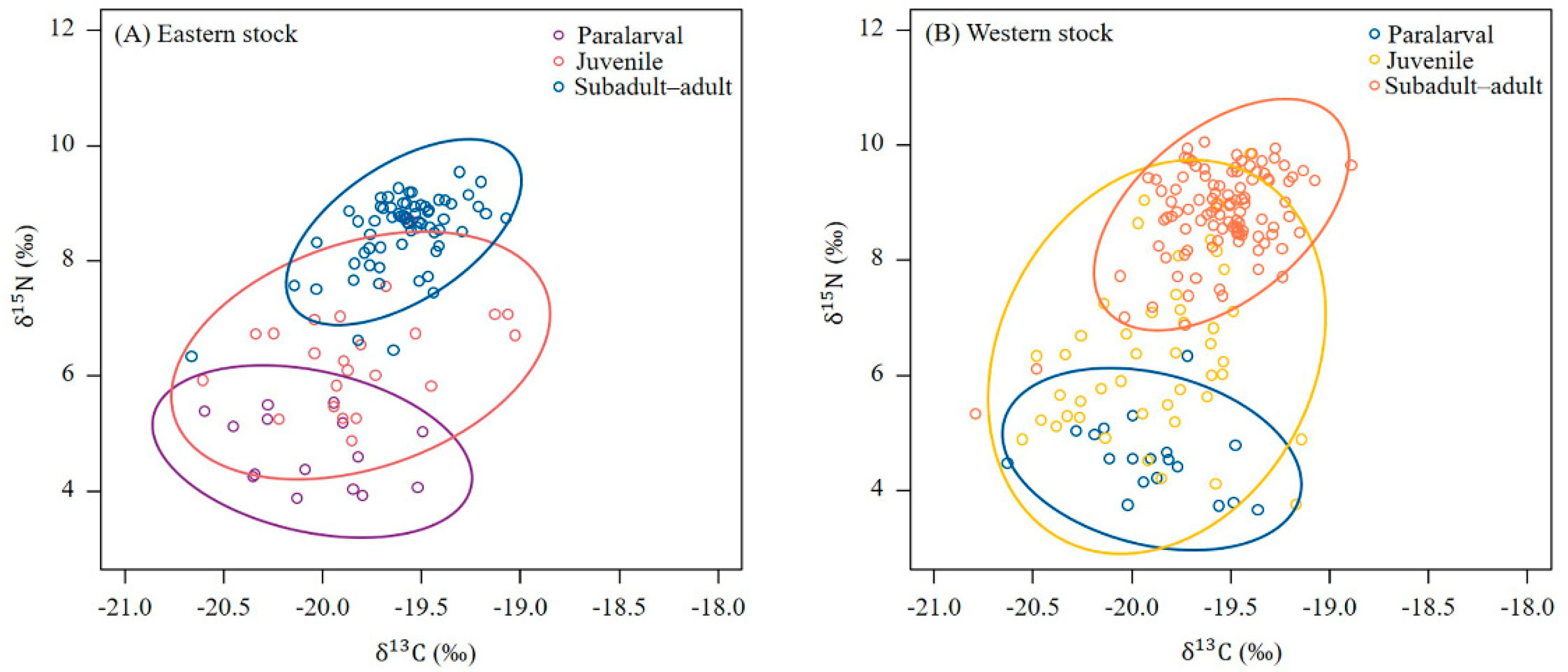
3.2. Distribution of Stable Isotope Values for the Eye Lenses

A total of 297 segments were extracted from 40 eye lenses. ${\mathsf{\delta }}^{13}\mathrm{C}$ values ranged from −21.04‰ to −18.89‰, and the ${\mathsf{\delta }}^{15}\mathrm{N}$ values from 3.67‰ to 12.27‰. Among them, there was a significant correlation between ${\mathsf{\delta }}^{15}\mathrm{N}$ and ${\mathsf{\delta }}^{13}\mathrm{C}$ values of successive segments of 19 individuals with positive correlation (p < 0.05). Only six specimens had a value of 3 for the ratio of ${\mathsf{\delta }}^{15}\mathrm{N}$ to ${\mathsf{\delta }}^{13}\mathrm{C}$ for the series of segments (

Table 3. Details of the linear relationship between δ¹⁵N and δ¹³C for the sampled O. bartramii eye lenses.

ID	N	δ13C/‰		δ15N/‰		δ15N/δ13C
		Mean ± SD	Range	Mean ± SD	Range	Slope	p-Value	R2
5	8	−19.81 ± 0.34	−20.38~−19.47	7.44 ± 1.59	4.56~9.13	4.083	0.05 *	0.753
9	7	−19.90 ± 0.17	−20.19~−19.68	7.93 ± 1.68	4.97~9.43	7.038	0.695	0.483
15	7	−19.78 ± 0.17	−20.19~−19.68	7.79 ± 0.51	4.89~9.64	2.978	0.001 **	0.904
19	6	−19.73 ± 0.30	−20.14~−19.40	8.32 ± 1.89	5.09~9.85	5.538	0.022 *	0.770
21	7	−19.66 ± 0.08	−19.78~−19.59	8.37 ± 1.64	5.19~10.06	6.784	0.487	0.101
24	6	−19.52 ± 0.33	−19.92~−19.08	8.02 ± 1.79	4.52~9.55	4.1	0.081	0.574
25	8	−19.66 ± 0.43	−20.66~−19.13	8.10 ± 0.87	6.34~8.88	1.152	0.143	0.322
37	8	−19.74 ± 0.44	−20.34~−19.20	7.60 ± 1.85	4.29~9.54	4.005	0.000 **	0.892
45	6	−19.80 ± 0.17	−20.16~−19.62	8.10 ± 1.17	5.77~9.05	5.956	0.018 *	0.789
48	7	−19.56 ± 0.20	−20.00~−19.46	7.50 ± 1.60	4.55~8.76	6.357	0.031 *	0.641
49	6	−19.56 ± 0.22	−19.85~−19.15	7.27 ± 1.75	4.22~9.07	5.841	0.087	0.560
56	7	−19.46 ± 0.09	−19.60~−19.33	7.46 ± 1.60	4.12~8.51	13.736	0.028 *	0.650
57	6	−19.62 ± 0.28	−20.13~−19.24	7.77 ± 1.64	4.92~9.30	4.294	0.098	0.536
71	7	−19.69 ± 0.26	−20.26~−19.49	6.99 ± 1.94	3.79~8.80	0.991	0.780	0.017
74	7	−19.62 ± 0.24	−19.95~−19.17	7.51 ± 1.97	3.76~9.54	−2.088	0.581	0.065
77	7	−19.86 ± 0.46	−20.63~−19.33	7.38 ± 1.71	4.49~9.52	3.715	0.000 **	0.989
91	8	−19.61 ± 0.23	−19.82~−19.06	8.06 ± 1.46	4.59~9.19	0.041	0.988	0.000
94	8	−19.91 ± 0.32	−20.45~−19.55	7.56 ± 1.51	5.12~9.09	4.365	0.001 **	0.836
95	9	−19.45 ± 0.17	−19.60~−19.03	8.03 ± 1.24	5.03~9.05	−2.361	0.407	0.100
100	7	−19.45 ± 0.09	−19.62~−19.34	7.53 ± 1.91	3.67~8.99	0.342	0.971	0.000
111	7	−19.54 ± 0.38	−19.87~−18.89	8.19 ± 1.83	4.22~9.65	2.823	0.170	0.339
113	7	−19.68 ± 0.13	−19.90~−19.47	8.23 ± 1.93	4.56~9.94	7.902	0.215	0.288
114	6	−19.57 ± 0.37	−20.33~−19.24	8.77 ± 1.66	5.29~9.94	3.545	0.059	0.632
118	7	−19.61 ± 0.43	−20.28~−19.20	7.90 ± 1.94	5.03~9.78	4.194	0.003 **	0.853
145	3	−19.59 ± 0.15	−19.80~−19.45	5.50 ± 1.17	3.92~6.74	6.725	0.345	0.734
152	5	−19.68 ± 0.24	−19.94~−19.29	6.6 ± 1.58	4.04~8.51	5.548	0.064	0.733
155	5	−19.83 ± 0.23	−20.13~−19.41	5.88 ± 1.49	3.88~8.25	5.897	0.021 *	0.869
158	5	−19.67 ± 0.42	−20.35~−19.07	6.43 ± 1.58	4.26~8.74	3.64	0.003 **	0.961
161	9	−19.78 ± 0.32	−20.60~−19.47	7.56 ± 1.41	5.40~9.11	3.053	0.040 *	0.475
172	6	−19.60 ± 0.32	−20.09~−19.26	7.47 ± 1.69	4.38~9.15	5.007	0.002 **	0.930
176	8	−19.81 ± 0.45	−20.60~−19.17	7.94 ± 1.15	5.93~9.26	2.26	0.004 **	0.779
178	8	−19.81 ± 0.27	−20.28~−19.54	8.03 ± 1.26	5.25~9.19	4.001	0.006 **	0.744
183	6	−19.59 ± 0.18	−19.82~−19.36	7.86 ± 1.97	4.54~9.77	2.795	0.624	0.066
186	5	−19.59 ± 0.21	−20.00~−19.39	7.84 ± 1.72	5.30~9.41	6.528	0.092	0.666
188	8	−19.72 ± 0.16	−20.02~−19.56	6.73 ± 2.17	3.74~9.16	6.626	0.207	0.25
189	7	−19.72 ± 0.49	−20.46~−19.21	7.28 ± 1.95	4.15~8.94	3.327	0.019 *	0.698
192	6	−19.70 ± 0.30	−20.26~−19.29	7.89 ± 1.19	5.55~8.94	3.439	0.031 *	0.728
204	7	−19.71 ± 0.14	−19.90~−19.52	7.05 ± 1.59	4.06~8.81	−0.502	0.927	0.002
207	8	−19.91 ± 0.51	−20.79~−19.14	6.22 ± 1.06	4.79~7.73	−0.384	0.663	0.034
214	8	−19.67 ± 0.23	−20.03~−19.35	7.93 ± 1.42	5.19~9.06	4.775	0.027 *	0.585

* shows that p < 0.05 and ** shows that p < 0.01; bolded numbers indicate these specimens closed to the expected value of 3 due to trophic enrichment.

).

3.3. Temporal and Spatial Differences between the Stable Isotope Values of the Different Squid Stocks

For the eastern stock, the ${\mathsf{\delta }}^{13}\mathrm{C}$ values in the lens segments were found to range from −20.60‰ to −19.49‰ (−20.06‰ ± 0.33‰), −20.60‰ to −19.03‰ (−19.81‰ ± 0.39‰) and −20.66‰ to −19.07‰ (−19.59‰ ± 0.24‰) for the paralarval, juvenile and subadult–adult stages, respectively. The corresponding ranges of the ${\mathsf{\delta }}^{15}\mathrm{N}$ values were 3.88‰ to 5.54‰ (4.70‰ ± 0.61‰), 4.87‰ to 8.71‰ (6.36‰ ± 0.88‰) and 6.34‰ to 9.54‰ (8.51‰ ± 0.66‰), respectively. The results of ANOVA showed significant differences in ${\mathsf{\delta }}^{13}\mathrm{C}$ and ${\mathsf{\delta }}^{15}\mathrm{N}$ values of different growth stages (F_C = 26.756, p_C < 0.05; F_N = 69.784, p_N < 0.05) (Figure 6;

Table 4. Stable isotope concentrations of neon flying squid eye lenses from the eastern and western stock populations (multiple comparisons by letters (a,b) to show significant differences (p < 0.05). SD represents standard deviation).

Group	Stage	δ13C/‰		δ15N/‰
		Mean ± SD	Range	Mean ± SD	Range
Western stock	Paralarvae	−19.90 ± 0.31 b	−20.63~−19.36	4.56 ± 0.64 b	3.67~6.34
	Juvenile	−19.88 ± 0.35 b	−20.55~−19.14	6.33 ± 1.39 b	3.76~9.85
	Subadult–adult	−19.55 ± 0.26 a	−20.79~−18.89	8.80 ± 0.82 a	5.33~10.06
Eastern stock	Paralarvae	−20.06 ± 0.33 b	−20.60~−19.49	4.70 ± 0.61 b	3.88~5.54
	Juvenile	−19.81 ± 0.39 b	−20.60~−19.03	6.36 ± 0.88 b	4.87~8.71
	Subadult–adult	−19.59 ± 0.24 a	−20.66~−19.07	8.51 ± 0.66 a	6.34~9.54

).

For the western squid stock, the ${\mathsf{\delta }}^{13}\mathrm{C}$ values in the lens segments were found to range from −20.63‰ to −19.36‰ (−19.90‰ ± 0.31‰), −20.55‰ to −19.14‰ (−19.88‰ ± 0.35‰) and −20.79‰ to −18.89‰ (−19.55‰ ± 0.26‰) for the paralarval, juvenile and subadult–adult stages, respectively. The corresponding ranges of ${\mathsf{\delta }}^{15}\mathrm{N}$ values were 3.67‰ to 6.34‰ (4.56‰ ± 0.64‰), 3.76‰ to 9.85‰ (6.33‰ ± 1.39‰) and 5.33‰ to 10.06‰ (8.80‰ ± 0.82‰), respectively. The results of ANOVA showed significant differences in ${\mathsf{\delta }}^{13}\mathrm{C}$ and ${\mathsf{\delta }}^{15}\mathrm{N}$ values of different growth stages (F_C = 43.769, p_C < 0.05; F_N = 102.968, p_N < 0.05) (Figure 6; Table 4).

With the comparison of the differences between the ${\mathsf{\delta }}^{13}\mathrm{C}$ and ${\mathsf{\delta }}^{15}\mathrm{N}$ values for the eastern and western squid stocks, it can be seen that there were no significant differences in the ${\mathsf{\delta }}^{13}\mathrm{C}$ and ${\mathsf{\delta }}^{15}\mathrm{N}$ values at the stage of paralarval and juvenile (p > 0.05), and at the stage of subadult–adult, the ${\mathsf{\delta }}^{15}\mathrm{N}$ values had significant difference between two stocks (F = 8.181, p < 0.05), while the opposite was true for ${\mathsf{\delta }}^{13}\mathrm{C}$ values (Figure 6). In addition, ANOVA showed no significant difference in ML between the two stocks (p > 0.05).

For the eastern stock, the SEAc values for the paralarval, juvenile and subadult–adult squid were 0.65‰², 1.06‰² and 0.43‰², respectively. There was a trophic separation between the paralarval and subadult–adult squid. There was a low amount of trophic overlap between the paralarval and juvenile, juveniles and subadult–adults, the corresponding values were 0.24 and 0.14, respectively, whereas there was a trophic separation between the paralarval and subadult–adult squid (Figure 7;

Table 5. Eastern and western stock trophic SEAc (‰²) and overlap in different growth stages.

Group	Stage	Paralarval	Juvenile	Subadult–Adult
Eastern stock	Paralarval	0.65‰2
	Juvenile	0.24	1.06‰2
	Subadult–adult	0.00	0.14	0.43‰2
Western stock	Paralarval	0.64‰2
	Juvenile	0.29	1.52‰2
	Subadult–adult	0.00	0.21	0.59‰2

).

For the western stock, the SEAc values for the paralarval, juvenile and subadult–adult squid were found to be 0.64‰², 1.52‰² and 0.59‰², respectively. There was a trophic separation between the paralarval and the subadult–adult squid. The trophic overlap ratio between paralarval and juveniles and that between juveniles and subadult–adults were 0.29 and 0.21, respectively (Figure 7; Table 5).

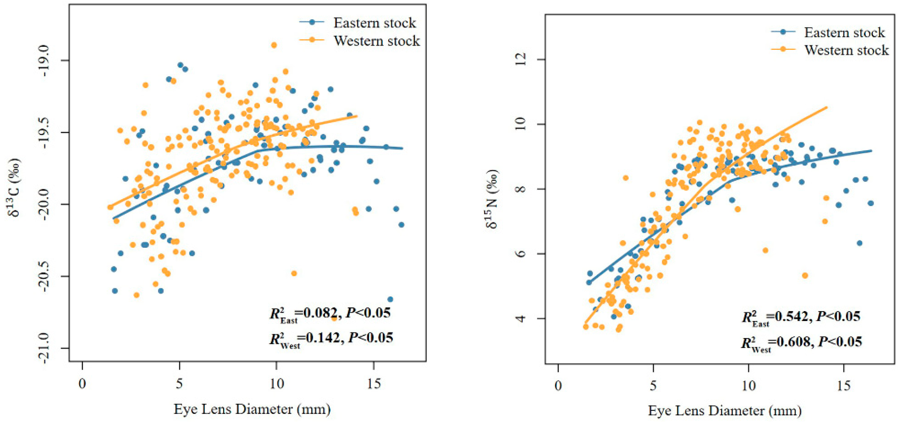
3.4. Assessment of the Suitability of Using Squid Eye Lenses to Determine the Ontogenetic Variation in Stable Isotope Values

Loess curves were constructed to show the variations in the stable carbon and nitrogen isotope values during squid ontogenesis based on the LDs and the stable carbon and nitrogen isotope values that were found for each eye lens segment (Figure 8). It can be seen that, for both squid stocks, both the ${\mathsf{\delta }}^{13}\mathrm{C}$ and ${\mathsf{\delta }}^{15}\mathrm{N}$ values increased significantly as LD increased (${\mathsf{\delta }}^{13}\mathrm{C}$: R²_West = 0.142, p < 0.05; R²_East = 0.082, p < 0.05; ${\mathsf{\delta }}^{15}\mathrm{N}$: R²_West = 0.608, p < 0.05; R²_East = 0.542, p < 0.05; Figure 8).

Loess curves showed that the ${\mathsf{\delta }}^{13}\mathrm{C}$ values of the western stock of squid were higher than those of the eastern stock. For both stocks, the growth rates of ${\mathsf{\delta }}^{13}\mathrm{C}$ values were similar in the early stage of the life cycle with the increase in LD. When LD was larger than about 8.95 mm, the ${\mathsf{\delta }}^{13}\mathrm{C}$ values of the eastern stock tended to be flattened, while the growth rate of ${\mathsf{\delta }}^{13}\mathrm{C}$ values decreased for the western stock after LD was larger than about 8.34 mm, but was still larger than that of the fall cohort (Figure 8).

In contrast, when the LD was less than about 6.03 mm, the ${\mathsf{\delta }}^{15}\mathrm{N}$ values of the eastern stock were greater than that of the western stock, while the ${\mathsf{\delta }}^{15}\mathrm{N}$ values of the western stock increased at a greater rate compared with the eastern stock in the early stage of individual development; when the LD was greater than about 7.82 mm and 8.87 mm, respectively, both the ${\mathsf{\delta }}^{15}\mathrm{N}$ values growth rate of the western and eastern stock decreased. However, the growth rate of the western squid stock remains higher than that of the eastern stock, which meant that the difference in the ${\mathsf{\delta }}^{15}\mathrm{N}$ values between the two stocks gradually widened (Figure 8).

4. Discussion

In the study of the changes in isotopic values over the life cycle of the individual squid, trophic effects should be considered; however, it is also necessary to consider whether variations in baseline values due to geographic migration influence the values. Moreno et al. [63] considered that ignoring the baseline values or using a single baseline for multiple geographical regions would distort the result. Actually, a value of 3:1 for the ratio of ${\mathsf{\delta }}^{15}\mathrm{N}$/${\mathsf{\delta }}^{13}\mathrm{C}$ with increases in trophic level is widely used in trophic stable isotope studies [64]; also, assuming that the squid does not move to a different geographic area during their lifetime, the ratio of trophic increase should remain close to 3:1 theoretically [41]. However, in this study, only a few specimens were found that had a ${\mathsf{\delta }}^{15}\mathrm{N}$/${\mathsf{\delta }}^{13}\mathrm{C}$ ratio that was similar to the theoretical value (Table 3), which meant that, for these squids, the ontogenetic isotopic variation was related not only to trophic growth but also to geographic movement. In addition, based on the feeding analysis of O. bartramii by Watanabe (2004) [9] and Watanabe (2008) [65], the winter–spring and fall cohorts fed mainly on fishes of Myctophidae and the feeding proportion of fish increased gradually as the individuals grew. Moreover, the winter–spring cohort also consumed fishes such as Engraulis japonicas and Maurolicus imperatorius, and cephalopods such as Watasenia scillallans, while the fall cohort consumed cephalopods such as Berryteuthis anonychus, Gonatus spp., Abraliopsis spp. and Onychoteuthis borealijaponica. Among them, Myctophidae, E. japonicas and cephalopods have geographic migratory behavior. For example, the larvae and fry of Myctophidae in the western North Pacific are mainly distributed in the western transient zone, and when the length reaches 40mm, fishes migrate northward to the Oyashio Current and involve in the Western Subarctic Gyre [66,67]. Therefore, migratory prey maybe have an effect on the ${\mathsf{\delta }}^{15}\mathrm{N}$/${\mathsf{\delta }}^{13}\mathrm{C}$ ratio variation during the growth and migration of individual predators.

In this study, both the ${\mathsf{\delta }}^{13}\mathrm{C}$ and ${\mathsf{\delta }}^{15}\mathrm{N}$ values of the eastern and western squid stocks presented an increasing trend throughout the life cycle (Figure 8). Similar results have been obtained for other hard structures found in O. bartramii, including beaks [68] and also obtained for gladii in jumbo squid (Dosidicus gigas) [69]. The ${\mathsf{\delta }}^{13}\mathrm{C}$ values increased continuously for both the eastern and western squid stocks during the ontogenetic growth of O. bartramii, which implied that they tended to migrate from lower baseline ${\mathsf{\delta }}^{13}\mathrm{C}$ values to higher baseline ${\mathsf{\delta }}^{13}\mathrm{C}$ values. Bower and Ichii [70] found that the North Pacific population of O. bartramii could be further divided into fall cohort (hatching period mainly from September to February) and winter–spring cohort (hatching period mainly from January to May, while it could be extended to August). In addition, the fall cohort mainly spread east of 170° E and near 160° W, while the majority of the winter–spring cohort was located west of 170° E [71]. In this study, based on the catching sites and hatching dates of the two stocks, it was finally determined that the western stock was the winter–spring cohort, while the eastern stock was the fall cohort. In fact, in the early stage of individual development, the STFZ where the fall cohort was located was close to the transition zone chlorophyll front (TZCF), thus bringing higher winter productivity for them, while the STD where the spawning ground of the winter–spring population was located was less productive. As the TZCF moved northward, the chlorophyll concentration in the TZ and SAFZ was higher, thus bringing greater productivity, so the migration of the winter–spring and fall cohorts from south to north during individual development was also a gradual movement to the high productivity zone [72]. Previous studies have suggested that male individuals of the fall cohort tended to stay in subtropical waters and did not migrate northward, but in this study, the sites where males were collected were located within the SAFZ, which meant that the males had some migration strategies [73]. However, due to the small sample size of male individuals, they cannot represent the whole stock. In addition, as noted above, migratory prey tends to consume different carbon sources, which could also contribute to the increase.

Furthermore, during ontogenesis, the ${\mathsf{\delta }}^{13}\mathrm{C}$ values of the western stock were higher than the eastern stock (Figure 8). The possible reason was that large- and mesoscale climatic and oceanic characteristics such as the Kuroshio Current and Oyashio Current dominate the influence over population dynamics of O. bartramii in the western North Pacific [74] and the Kuroshio and Oyashio Current are also significant sources of primary production for O. bartramii fishing grounds [75]; by contrast, in the eastern North Pacific, due to the offshore trade winds, upwelling occurs in the California Current and in the region, most of the year it occurs strong offshore surface transport [76]. In addition, Fang (2016) [77] showed that compared with the western stock, the eastern stock was farther from shore, which was assumed in this study to result in lower ${\mathsf{\delta }}^{13}\mathrm{C}$ values in the eastern stock of O. bartramii during migration than the western stock.

Similar to the trends in the ${\mathsf{\delta }}^{13}\mathrm{C}$ values, in this study, the ${\mathsf{\delta }}^{15}\mathrm{N}$ values of both western and eastern stocks of O. bartramii were found to continuously increase from the paralarval to the subadult–adult stage (Figure 8). In the squid-occupied ocean, if the effects of trophic variation during ontogenetic growth were excluded, during the progressive formation of eye lenses, there would be a systematic decrease in ${\mathsf{\delta }}^{15}\mathrm{N}$ values, which was often associated with habitat shifts during migration and was evidenced by a decrease in baseline ${\mathsf{\delta }}^{15}\mathrm{N}$ values, according to Somes et al. (2010) [78]. However, it is contrary to the results of this study. In addition, there was a significant correlation between ${\mathsf{\delta }}^{15}\mathrm{N}$ values and LD for both stocks in this study. Here, we suggest that as the squids undergo ontogenetic growth, their beak sizes get gradually larger, which means that they can feed on prey with greater body length and from higher trophic levels, including fish and other cephalopods [79,80]; thus, there is a shift from lower to higher trophic levels as they grow. Fang et al. (2016) [68] noted that the differences between two stocks are often related to differences in population growth rates, composition of feeding food and migration routes. When the LD was less than about 6.03 mm, the ${\mathsf{\delta }}^{15}\mathrm{N}$ values of the eastern stock were greater than that of the western stock, and individuals in the LD range were basically in the paralarval–juvenile stage. Ichii et al. [19] showed that in the early stage of the life cycle, the growth rate of the fall cohort was faster compared to winter-spring populations, which therefore meant that they were able to feed on higher trophic level prey earlier and thus had higher ${\mathsf{\delta }}^{15}\mathrm{N}$ values. In the later stages of individual development, the difference in ${\mathsf{\delta }}^{15}\mathrm{N}$ values between the two stocks increased. While in the later stages of growth, the fall cohort grew less rapidly than the winter-spring cohort, which had an effect on ${\mathsf{\delta }}^{15}\mathrm{N}$ values. In addition based on the diet composition consumed by the two stocks described above, it was found that although their trophic levels were essentially similar, the differences in feeding composition brought about by geographical differences between the two stocks could also have some influence on ${\mathsf{\delta }}^{15}\mathrm{N}$ values, as O. bartramii are opportunistic, voracious predators. In addition, the variation in baseline values of different geographic regions during the migration of the two stocks would also be reflected in the variation of ${\mathsf{\delta }}^{15}\mathrm{N}$ values.

Multiple comparisons showed that ${\mathsf{\delta }}^{13}\mathrm{C}$ and ${\mathsf{\delta }}^{15}\mathrm{N}$ values were significantly different between the paralarval–juvenile and subadult–adult stages of both stocks, but not between the paralarval and juvenile stage (Table 4). We suggest that the significant difference in ${\mathsf{\delta }}^{13}\mathrm{C}$ values could be explained by geographic differences, as the habitat during the paralarval–juvenile stage was less diverse, squid were initially concentrated in the southern spawning ground and then started to move northward, while the significant differences in ${\mathsf{\delta }}^{15}\mathrm{N}$ values were often related to differences in food composition in different areas and the size of ML. For eastern and western stocks, within each growth stage, we observed that the variability in the ${\mathsf{\delta }}^{15}\mathrm{N}$ values was higher in the juvenile stage (western stock: 6.09‰; eastern stock: 3.84‰) (Figure 6). It is usually considered that the range of ${\mathsf{\delta }}^{15}\mathrm{N}$ values (NR) reflects the trophic length that is occupied by the squid: the larger the NR, the more trophic levels that are occupied [58]. O. bartramii is a voracious, opportunistic predator [81]; thus, at the juvenile stages, for the western stock, the Kuroshio Current and Oyashio Current bring rich and different trophic levels of food resources for the squid to obtain; for the eastern stock, the spawning ground has abundant feeding resources due to their proximity to TZCF [82]. However, later in the life cycle of the squid, as a result of the increase in mantle length and migration to its feeding grounds, O. bartramii may have a preference for larger prey from higher trophic levels. The breadth of the food resources then decreases, which causes the NR of O. bartramii in the later stages of the life cycle to decrease. This phenomenon can also be observed for some fish and other cephalopod species [83,84].

Niches not only reflect the spatial position occupied by a species within a certain environmental range at a certain time, but also reflect the influence of environmental and other factors on the species [85]. The niche breadth reflects the diversity or uniformity of species’ feeding resources: the greater the breadth, the greater the environmental adaptability of the species. The niche overlap is another important indicator to measure the degree of competition and the similarity of resource utilization between or within species at different periods [86,87].

In this study, we focused on the niche variation of squid exogenous feeding after hatching. For both the eastern and western stocks, the SEAc values peak at the juvenile stage, which suggests that there is some variation in the resources used for ontogenetic growth [88]. Many species use similar resources when small [89]. At the paralarval stage, the swimming ability of O. bartramii is poor and their main source of food is plankton; thus, given the predation risk, the individual squid prefers to rely on similar resources and has a low adaptive capacity to the environment. Later, as a result of their ontogenetic growth, the squid tends to migrate to more open habitats, and the amount of diversity in the isotopic niches that they occupy increases [90]. According to previous studies, we found that, after the entry of the juvenile stage, the swimming ability of the squid improves as they migrate into the open water [91]. Their food sources then become more diverse due to the interaction between different ecosystems: their feeding targets are no longer limited to plankton and begin to shift toward small fish and other cephalopods [9,65]. This explains the larger SEAc values found for the juvenile stage of O. bartramii. For both stocks, the SEAc values first increase and then decline. Similar to the trends in NR discussed above, the SEAc values decrease in the later life stages. In their investigation of shark niches, Bethea et al. [92] pointed out that a reduction in the size of the niche may be due to larger individuals focusing more on specialized prey. Given the migratory activity of O. bartramii, this strengthens the conclusion that, in the later stages of their life cycle when they migrate to their feeding grounds, O. bartramii with larger ML focus more on larger prey (Figure 7).

The ${\mathsf{\delta }}^{13}\mathrm{C}$ and ${\mathsf{\delta }}^{15}\mathrm{N}$ values found for eye lenses suggest that for both the eastern and western stocks in the early stage of their life cycle, the amount of overlap in the SEAc between squid at the paralarval and juvenile stages was low (0.29 for the western stock and 0.24 for the eastern stock) (Table 5). This was followed by a continuous decrease in the overlap between the juvenile and subadult–adult stages (western stock: juvenile/subadult–adult: 0.21; eastern stock: juvenile/subadult–adult: 0.14), indicating that there is a gradual trophic niche separation between paralarval–juvenile and subadult–adult squid. This separation is related to changes in the O. bartramii habitat and influencing factors throughout its life cycle, exactly as Camarillo-Coop et al. [93] suggested that, as the size of the squid increases, so does the amount and variety of their prey, and that a gradual shift from small to large prey also leads to changes in the niche occupied by the squid [94].

5. Conclusions and Prospects

In this study, in the light of combined information from statolith determined age and stable eye lens isotopes, together with details of the squid life cycle and interactions with environment, we conclude the ontogenetic changes in their trophic preference and the O. bartramii collected were sexually immature, which meant that these individuals could not fully demonstrate the trophic variation that O. bartramii exhibited during the life cycle. In future studies, we will aim to carry out more comprehensive sampling to reduce the influence of this factor on the study results, and we will also aim to explore the trophic influence of North Pacific O. bartramii on other fishery organisms in the North Pacific Ocean, as well as the influence on the North Pacific ecosystem based on climatic and fishery conditions.

References

1. Roper, C.F.; Sweeney, M.J.; Nauen, C.E. Cephalopods of the World. An Annotated and Illustrated Catalogue of Species of Interest to Fisheries; United Nations Development Programme, Food and Agriculture Organization of the United Nations: Rome, Italy, 1984; Volume 3, pp. 1–277. [Google Scholar]
2. Murata, M. On the flying behavior of neon flying squid Ommastrephes bartramii observed in the central and northwestern north pacific. Nippon Suisan Gakkaishi. 1988, 54, 1167–1174. [Google Scholar] [CrossRef]
3. Murata, M. Oceanic resources of squids. Mar. Freshw. Behav. Phy. 1990, 18, 19–71. [Google Scholar] [CrossRef]
4. Murata, M. Life history and biological information on flying squid (Ommastrephes bartramii) in the North Pacific Ocean. Bull. Int. Nat. North Pac. Comm. 1993, 53, 147–182. [Google Scholar]
5. Xu, J.; Chen, X.; Chen, Y.; Ding, Q.; Tian, S. The effect of sea surface temperature increase on the potential habitat of Ommastrephes bartramii in the Northwest Pacific Ocean. Acta Ocean. Sin. 2016, 35, 109–116. [Google Scholar] [CrossRef]
6. Vijai, D.; Sakai, M.; Wakabayashi, T.; Yoo, H.K.; Kato, Y.; Sakurai, Y. Effects of temperature on embryonic development and paralarval behavior of the neon flying squid Ommastrephes bartramii. Mar. Ecol. Prog. Ser. 2015, 529, 145–158. [Google Scholar] [CrossRef]
7. Wang, J.; Yu, W.; Chen, X.; Lei, L.; Chen, Y. Detection of potential fishing zones for neon flying squid based on remote-sensing data in the Northwest Pacific Ocean using an artificial neural network. Int. J. Remote Sens. 2015, 36, 3317–3330. [Google Scholar] [CrossRef]
8. Nigmatullin, C.M.; Shchetinnikov, A.S.; Shukhgalter, O.A. On feeding and helminth fauna of neon flying squid Ommastrephes bartramii (Lesueur, 1821) (Cephalopoda: Ommastrephidae) in the southeastern Pacific. Rev. De Biol. Mar. Y Oceanogr. 2009, 44, 227–235. [Google Scholar] [CrossRef] [Green Version]
9. Watanabe, H.; Kubodera, T.; Ichii, T.; Kawahara, S. Feeding habits of neon flying squid Ommastrephes bartramii in the transitional region of the central North Pacific. Mar. Ecol. Prog. Ser. 2004, 266, 173–184. [Google Scholar] [CrossRef] [Green Version]
10. Seki, M.P.; Polovina, J.J.; Kobayashi, D.R.; Bidigare, R.R.; Mitchum, G.T. An oceanographic characterization of swordfish (Xiphias gladius) longline fishing grounds in the springtime subtropical North Pacific. Fish Oceanogr. 2002, 11, 251–266. [Google Scholar] [CrossRef] [Green Version]
11. Clarke, M.R.; Roeleveld, M.A.C. Cephalopods in the diet of sperm whales caught commercially off Durban, South Africa. Afr. J. Mar. Sci. 1998, 20, 41–45. [Google Scholar] [CrossRef] [Green Version]
12. Yu, W.; Chen, X.; Yi, Q. Fishing ground distribution of neon flying squid (Ommastrephes bartramii) in relation to oceanographic conditions in the northwest Pacific Ocean. J. Ocean Univ. China 2017, 16, 1157–1166. [Google Scholar] [CrossRef]
13. Chen, C.S.; Chiu, T.S. Variations of life history parameters in two geographical groups of the neon flying squid, Ommastrephes bartramii, from the North Pacific. Fish Res. 2003, 63, 349–366. [Google Scholar] [CrossRef]
14. Yatsu, A.; Tanaka, H.; Mori, J. Population structure of the neon flying squid, Ommastrephes bartramii, in the North Pacific Ocean. In Contributed Papers to International Symposium on Large Pelagic Squids, 18–19 July 1996, for JAMARC’s 25th Anniversary of its Foundation; Japan Marine Fishery Resources Research Center: Tokyo, Japan, 1998; pp. 31–48. [Google Scholar]
15. Chen, X.; Tian, S.; Liu, B.; Chen, Y. Modeling a habitat suitability index for the eastern fall cohort of Ommastrephes bartramii in the central North Pacific Ocean. Chin. J. Ocean. Limnol. 2011, 29, 493–504. [Google Scholar] [CrossRef]
16. Yu, W.; Chen, X.; Yi, Q.; Gao, G.; Chen, Y. Impacts of climatic and marine environmental variations on the spatial distribution of Ommastrephes bartramii in the Northwest Pacific Ocean. Acta Ocean. Sin. 2016, 35, 108–116. [Google Scholar] [CrossRef]
17. Golikov, A.V.; Ceia, F.R.; Sabirov, R.M.; Zaripova, Z.I.; Blicher, M.E.; Zakharov, D.V.; Xavier, J.C. Ontogenetic changes in stable isotope (δ13C and δ15N) values in squid Gonatus fabricii (Cephalopoda) reveal its important ecological role in the Arctic. Mar. Ecol. Prog. Ser. 2018, 606, 65–78. [Google Scholar] [CrossRef]
18. Yu, W.; Chen, X.; Zhang, Y.; Yi, Q. Habitat suitability modelling revealing environmental-driven abundance variability and geographical distribution shift of winter–spring cohort of neon flying squid Ommastrephes bartramii in the northwest Pacific Ocean. ICES J. Mar. Sci. 2019, 76, 1722–1735. [Google Scholar] [CrossRef]
19. Ichii, T.; Mahapatra, K.; Sakai, M.; Okada, Y. Life history of the neon flying squid: Effect of the oceanographic regime in the North Pacific Ocean. Mar. Ecol. Prog. Ser. 2009, 378, 1–11. [Google Scholar] [CrossRef]
20. Hobson, K.A. Tracing origins and migration of wildlife using stable isotopes: A review. Oecologia 1999, 120, 314–326. [Google Scholar] [CrossRef]
21. McCutchan, J.H., Jr.; Lewis, W.M., Jr.; Kendall, C.; McGrath, C.C. Variation in trophic shift for stable isotope ratios of carbon, nitrogen, and sulfur. Oikos 2003, 102, 378–390. [Google Scholar] [CrossRef]
22. Kelly, M.H.; Hagar, W.G.; Jardine, T.D.; Cunjak, R.A. Nonlethal sampling of sunfish and slimy sculpin for stable isotope analysis: How scale and fin tissue compare with muscle tissue. N. Am. J. Fish. Manag. 2006, 26, 921–925. [Google Scholar] [CrossRef]
23. Cherel, Y.; Hobson, K.A. Geographical variation in carbon stable isotope signatures of marine predators: A tool to investigate their foraging areas in the Southern Ocean. Mar. Ecol. Prog. Ser. 2007, 329, 281–287. [Google Scholar] [CrossRef]
24. Minagawa, M.; Wada, E. Stepwise enrichment of 15N along food chains: Further evidence and the relation between δ15N and animal age. Geochim. Et Cosmochim. Acta. 1984, 48, 1135–1140. [Google Scholar] [CrossRef]
25. Jennings, S.; Warr, K.J. Environmental correlates of large-scale spatial variation in the δ15N of marine animals. Mar. Biol. 2003, 142, 1131–1140. [Google Scholar] [CrossRef]
26. Tanaka, Y.; Minami, H.; Ishihi, Y.; Kumon, K.; Higuchi, K.; Eba, T.; Nishi, A.; Nikaido, H.; Shiozawa, S. Relationship between prey utilization and growth variation in hatchery-reared Pacific bluefin tuna, Thunnus orientalis (Temminck et Schlegel), larvae estimated using nitrogen stable isotope analysis. Aquac. Res. 2014, 45, 537–545. [Google Scholar] [CrossRef]
27. Hesslein, R.H.; Hallard, K.A.; Ramlal, P. Replacement of sulfur, carbon, and nitrogen in tissue of growing broad whitefish (Coregonus nasus) in response to a change in diet traced by δ34S, δ13C, and δ15N. Can. J. Fish. Aquat. Sci. 1993, 50, 2071–2076. [Google Scholar] [CrossRef]
28. Gratton, C.; Forbes, A.E. Changes in δ 13C stable isotopes in multiple tissues of insect predators fed isotopically distinct prey. Oecologia 2006, 147, 615–624. [Google Scholar] [CrossRef]
29. Inger, R.; Bearhop, S. Applications of stable isotope analyses to avian ecology. Ibis 2008, 150, 447–461. [Google Scholar] [CrossRef]
30. Malpica-Cruz, L.; Herzka, S.Z.; Sosa-Nishizaki, O.; Lazo, J.P. Tissue-specific isotope trophic discrimination factors and turnover rates in a marine elasmobranch: Empirical and modeling results. Can. J. Fish. Aquat. Sci. 2012, 69, 551–564. [Google Scholar] [CrossRef]
31. Kato, Y.; Sakai, M.; Nishikawa, H.; Igarashi, H.; Ishikawa, Y.; Vijai, D.; Sakurai, Y.; Wakabayshi, T.; Awaji, T. Stable isotope analysis of the gladius to investigate migration and trophic patterns of the neon flying squid (Ommastrephes bartramii). Fish Res. 2016, 173, 169–174. [Google Scholar] [CrossRef]
32. Guerra, A.; Rodriguez-Navarro, A.B.; González, Á.F.; Romanek, C.S.; Alvarez-Lloret, P.; Pierce, G.J. Life-history traits of the giant squid Architeuthis dux revealed from stable isotope signatures recorded in beaks. ICES J. Mar. Sci. 2010, 67, 1425–1431. [Google Scholar] [CrossRef] [Green Version]
33. Quaeck, K. Stable Isotope Analysis of Fish Eye Lenses: Reconstruction of Ontogenetic Trends in Spatial and Trophic Ecology of Elasmobranchs and Deep-Water Teleosts. Ph.D. Thesis, University of Southampton, Southampton, UK, 2017. [Google Scholar]
34. Campana, S.E. Chemistry and composition of fish otoliths: Pathways, mechanisms and applications. Mar. Ecol. Prog. Ser. 1999, 188, 263–297. [Google Scholar] [CrossRef]
35. Trueman, C.N.; MacKenzie, K.M.; Palmer, M.R. Stable isotopes reveal linkages between ocean climate, plankton community dynamics, and survival of two populations of Atlantic salmon (Salmo salar). ICES J. Mar. Sci. 2012, 69, 784–794. [Google Scholar] [CrossRef]
36. Tzadik, O.E.; Curtis, J.S.; Granneman, J.E.; Kurth, B.N.; Pusack, T.J.; Wallace, A.A.; Hollander, D.J.; Peebles, E.B.; Stallings, C.D. Chemical archives in fishes beyond otoliths: A review on the use of other body parts as chronological recorders of microchemical constituents for expanding interpretations of environmental, ecological, and life-history changes. Limnol. Oceanogr. Methods 2017, 15, 238–263. [Google Scholar] [CrossRef]
37. Xu, W.; Chen, X.; Liu, B.; Chen, Y.; Huan, M.; Liu, N.; Lin, J. Inter-individual variation in trophic history of Dosidicus gigas, as indicated by stable isotopes in eye lenses. Aquac. Fish. 2019, 4, 261–267. [Google Scholar] [CrossRef]
38. Quaeck-Davies, K.; Bendall, V.A.; MacKenzie, K.M.; Hetherington, S.; Newton, J.; Trueman, C.N. Teleost and elasmobranch eye lenses as a target for life-history stable isotope analyses. PeerJ 2018, 6, e4883. [Google Scholar] [CrossRef]
39. Hunsicker, M.E.; Essington, T.E.; Aydin, K.Y.; Ishida, B. Predatory role of the commander squid Berryteuthis magister in the eastern Bering Sea: Insights from stable isotopes and food habits. Mar. Ecol. Prog. Ser. 2010, 415, 91–108. [Google Scholar] [CrossRef] [Green Version]
40. Onthank, K.L. Exploring the Life Histories of Cephalopods Using Stable Isotope Analysis of An Archival Tissue; Washington State University: Washington, DC, USA, 2013. [Google Scholar]
41. Meath, B.; Peebles, E.B.; Seibel, B.A.; Judkins, H. Stable isotopes in the eye lenses of Doryteuthis plei (Blainville 1823): Exploring natal origins and migratory patterns in the eastern Gulf of Mexico. Cont. Shelf. Res. 2019, 174, 76–84. [Google Scholar] [CrossRef]
42. Miserez, A.; Schneberk, T.; Sun, C.; Zok, F.W.; Waite, J.H. The transition from stiff to compliant materials in squid beaks. Science 2008, 319, 1816–1819. [Google Scholar] [CrossRef] [Green Version]
43. Arkhipkin, A.; Perez, J.A.A. Life history reconstruction. In Squid Recruitment Dynamics; United Nations Development Programme, Food and Agriculture Organization of the United Nations: Rome, Italy, 1998; pp. 157–180. [Google Scholar]
44. Xu, W.; Liu, B.; Chen, X.; Huan, M. Research advancements on role of eye lens in reconstruction of cephalopod life history. J. Dalian Fish. Univ. 2018, 33, 408–412. (In Chinese) [Google Scholar] [CrossRef]
45. Arkhipkin, A.I. Statoliths as ‘black boxes’(life recorders) in squid. Mar. Freshw. Res. 2005, 56, 573–583. [Google Scholar] [CrossRef]
46. Rodhouse, P.G.; Hatfield, E.M.C. Age determination in squid using statolith growth increments. Fish Res. 1990, 8, 323–334. [Google Scholar] [CrossRef]
47. Anken, R.H.; Werner, K.; Ibsch, M.; Rahmann, H. Fish inner ear otolith size and bilateral asymmetry during development. Hear. Res. 1998, 121, 77–83. [Google Scholar] [CrossRef]
48. Saito, T.; Kaga, T.; Seki, J.; Otake, T. Otolith microstructure of chum salmon Oncorhynchus keta: Formation of sea entry check and daily deposition of otolith increments in seawater conditions. Fish. Sci. 2007, 73, 27–37. [Google Scholar] [CrossRef]
49. Bigelow, K.A.; Landgraf, K.C. Hatch Dates and Growth of Ommastrephes bartramii Paralarvae from Hawaiian Waters as Determined from Statolith Analysis. In Recent Advances in Cephalopod Fisheries Biology; Tokai University Press: Tokyo, Japan, 1993; pp. 15–24. [Google Scholar]
50. Parry, M. Trophic variation with length in two ommastrephid squids, Ommastrephes bartramii and Sthenoteuthis oualaniensis. Mar. Biol. 2008, 153, 249–256. [Google Scholar] [CrossRef]
51. Wang, Y.; Han, P.; Chen, X.; Fang, Z. Interannual and ontogenetic stage differences on trophic ecology of neon flying squid Ommastrephes bartramii inferred from stable isotope analyses in beaks. Fish Res. 2022, 249, 106252. [Google Scholar] [CrossRef]
52. Ehrhardt, N.M. On the fishery and biology of the giant squid Dosidicus gigas in the Gulf of California, Mexico, in ”Advanced in Assessment of World Cephalopod Resources”. FAO Fish. Tech. Pap. 1983, 231, 306–339. [Google Scholar]
53. Dawe, E.G.; Natsukari, Y. Light microscopy. In Squid Age Determination Using Statoliths, Proceedings of the International Workshop, Mazara del Vallo, Italy, 9–14 October 1989; Jereb, P., Ragonese, S., BoletzkyVon, S., Eds.; Instituto di Tecnologiadella Pesca e del Pescato: Mazara del Vallo, Italy, 1991; pp. 83–96, NTR–ITPP Special Publications, No. 1. [Google Scholar]
54. Uozumi, Y.; Ohara, H. Age and Growth of Nototodarus sloanii (Cephalopoda: Oegopsida) Based on Daily Increment Counts in Statoliths. Nippon Suisan Gakkaishi 1993, 59, 1469–1477. [Google Scholar] [CrossRef]
55. Jin, Y.; Lin, F.; Chen, X.; Liu, B.; Li, J. Microstructure comparison of hard tissues (statoliths, beaks, and eye lenses) of Uroteuthis chinensis in the South China Sea. Bull. Mar. Sci. 2019, 95, 13–26. [Google Scholar] [CrossRef]
56. Liu, B.; Chen, X.; Zhong, J. Age, growth and population strcture of squid Sthenoteuthis oualaniensis in northwest Indian Ocean by statolith microstructure. Chin. J. Dalian Fish. Univ. 2009, 24, 206–212. (In Chinese) [Google Scholar] [CrossRef]
57. Post, D.M.; Layman, C.A.; Arrington, D.A.; Takimoto, G.; Quattrochi, J.; Montana, C.G. Getting to the fat of the matter: Models, methods and assumptions for dealing with lipids in stable isotope analyses. Oecologia 2007, 152, 179–189. [Google Scholar] [CrossRef]
58. Jackson, A.L.; Inger, R.; Parnell, A.C.; Bearhop, S. Comparing isotopic niche widths among and within communities: SIBER–Stable Isotope Bayesian Ellipses in R. J Anim. Ecol. 2011, 80, 595–602. [Google Scholar] [CrossRef] [PubMed]
59. R Core Team. R: A Language and Environment for Statistical Computing; R Foundation for Statistical Computing: Vienna, Austria, 2022. [Google Scholar]
60. Layman, C.A.; Arrington, D.A.; Montaña, C.G.; Post, D.M. Can stable isotope ratios provide for community-wide measures of trophic structure? Ecology 2007, 88, 42–48. [Google Scholar] [CrossRef]
61. Layman, C.A.; Araujo, M.S.; Boucek, R.; Hammerschlag-Peyer, C.M.; Harrison, E.; Jud, Z.R.; Matich, P.; Rosenblatt, A.E.; Vaudo, J.J.; Yeager, L.A.; et al. Applying stable isotopes to examine food-web structure: An overview of analytical tools. Biol. Rev. 2012, 87, 545–562. [Google Scholar] [CrossRef] [PubMed]
62. Langton, R.W. Diet overlap between Atlantic cod, Gadus morhua, silver hake, Merluccius bilinearis, and fifteen other northwest Atlantic finfish. Fish. Bull. 1982, 80, 45–759. [Google Scholar]
63. Moreno, R.; Jover, L.; Velando, A.; Munilla, I.; Sanpera, C. Influence of trophic ecology and spatial variation on the isotopic fingerprints of seabirds. Mar. Ecol. Prog. Ser. 2011, 442, 229–239. [Google Scholar] [CrossRef] [Green Version]
64. Faletti, M.E.; Stallings, C.D. Life history through the eyes of a hogfish: Trophic growth and differential juvenile habitat use from stable isotope analysis. Mar. Ecol. Prog. Ser. 2021, 666, 183–202. [Google Scholar] [CrossRef]
65. Watanabe, H.; Kubodera, T.; Ichii, T.; Sakai, M.; Moku, M.; Seitou, M. Diet and sexual maturation of the neon flying squid Ommastrephes bartramii during autumn and spring in the Kuroshio–Oyashio transition region. J. Mar. Biol. Assoc. UK 2008, 88, 381–389. [Google Scholar] [CrossRef]
66. Sassa, C.; Moser, H.G.; Kawaguchi, K. Horizontal and vertical distribution patterns of larval myctophid fishes in the Kuroshio Current region. Fish. Oceanogr. 2002, 11, 1–10. [Google Scholar] [CrossRef]
67. Moku, M.; Tsuda, A.; Kawaguchi, K. Spawning season and migration of the myctophid fish Diaphus theta in the western North Pacific. Ichthyol. Res. 2003, 50, 0052–0058. [Google Scholar] [CrossRef]
68. Fang, Z.; Thompson, K.; Jin, Y.; Chen, X.; Chen, Y. Preliminary analysis of beak stable isotopes (δ13C and δ15N) stock variation of neon flying squid, Ommastrephes bartramii, in the North Pacific Ocean. Fish. Res. 2016, 177, 153–163. [Google Scholar] [CrossRef] [Green Version]
69. Lorrain, A.; Argüelles, J.; Alegre, A.; Bertrand, A.; Munaron, J.M.; Richard, P.; Cherel, Y. Sequential isotopic signature along gladius highlights contrasted individual foraging strategies of jumbo squid (Dosidicus gigas). PLoS ONE 2011, 6, e22194. [Google Scholar] [CrossRef] [PubMed] [Green Version]
70. Bower, J.R.; Ichii, T. The red flying squid (Ommastrephes bartramii): A review of recent research and the fishery in Japan. Fish. Res. 2005, 76, 39–55. [Google Scholar] [CrossRef]
71. Chen, P.; Fang, Z.; Chen, X. Population identification of Ommastrephes bartramii based on beak’s external morphological characters. Mar. Fish. 2015, 37, 1–9. (In Chinese) [Google Scholar] [CrossRef]
72. Ichii, T.; Mahapatra, K.; Sakai, M.; Inagake, D.; Okada, Y. Differing body size between the autumn and the winter–spring cohorts of neon flying squid (Ommastrephes bartramii) related to the oceanographic regime in the North Pacific: A hypothesis. Fish Oceanogr. 2004, 13, 295–309. [Google Scholar] [CrossRef]
73. Yatsu, A.; Midorikawa, S.; Shimada, T.; Uozumi, Y. Age and growth of the neon flying squid, Ommastrephes bartramii, in the North Pacific Ocean. Fish. Res. 1997, 29, 257–270. [Google Scholar] [CrossRef]
74. Yu, W.; Chen, X.; Yi, Q.; Tian, S. A review of interaction between neon flying squid (Ommastrephes bartramii) and oceanographic variability in the North Pacific Ocean. J. Ocean Univ. China 2015, 14, 739–748. [Google Scholar] [CrossRef]
75. Wang, W.; Shao, Q.; Xue, Y.; Ji, T. On the relationship between the resources of Ommastrephes bartrami and marine environment in the Northwest Pacific Ocean based on GIS. J. Geogr. Inf. Sci. 2003, 5, 39–44. [Google Scholar]
76. Parrish, R.H.; Nelson, C.S.; Bakun, A. Transport mechanisms and reproductive success of fishes in the California Current. Biol. Oceanogr. 1981, 1, 175–203. [Google Scholar] [CrossRef]
77. Fang, Z. Fisheries Ecology of Neon Flying Squid Ommastrephes bartramii in North Pacific Ocean based on beak. Ph.D. Thesis, University of Shanghai Ocean, Shanghai, China, 2016. [Google Scholar]
78. Somes, C.J.; Schmittner, A.; Galbraith, E.D.; Lehmann, M.F.; Altabet, M.A.; Montoya, J.P.; Letelier, R.M.; Mix, A.C.; Bourbonnais, A.; Eby, M. Simulating the global distribution of nitrogen isotopes in the ocean. Glob. Biogeochem. Cycles 2010, 24, GB4019. [Google Scholar] [CrossRef]
79. Parry, M. Feeding behavior of two ommastrephid squids Ommastrephes bartramii and Sthenoteuthis oualaniensis off Hawaii. Mar. Ecol. Prog. Ser. 2006, 318, 229–235. [Google Scholar] [CrossRef]
80. Jin, Y.; Chen, X. Information in beaks of Ommastrephes bartramii in the North Pacific Ocean using stable isotope technology. Chin. J. Ecology 2014, 33, 2101–2107, (In Chinese with English Abstract). [Google Scholar] [CrossRef]
81. Rodhouse, P.G.; Nigmatullin, C.M. Role as consumers. Philos. Trans. R. Soc. Lond. Ser. B Biol. Sci. 1996, 351, 1003–1022. [Google Scholar] [CrossRef]
82. Ichii, T.; Mahapatra, K.; Sakai, M.; Wakabayashi, T.; Okamura, H.; Igarashi, H.; Inagake, D.; Okada, Y. Changes in abundance of the neon flying squid Ommastrephes bartramii in relation to climate change in the central North Pacific Ocean. Mar. Ecol. Prog. Ser. 2011, 441, 151–164. [Google Scholar] [CrossRef] [Green Version]
83. Sauer, W.H.H.; Lipiński, M.R. Food of squid Loligo vulgaris reynaudii (Cephalopoda: Loliginidae) on their spawning grounds off the Eastern Cape, South Africa. S. Afr. J. Mar. Sci. 1991, 10, 193–201. [Google Scholar] [CrossRef]
84. Carlisle, A.B.; Goldman, K.J.; Litvin, S.Y.; Madigan, D.J.; Bigman, J.S.; Swithenbank, A.M.; Kline, T.C.; Block, B.A. Stable isotope analysis of vertebrae reveals ontogenetic changes in habitat in an endothermic pelagic shark. Proc. R. Soc. B-Biol. Sci. 2015, 282, 20141446. [Google Scholar] [CrossRef]
85. Zhang, G.; Xie, S.C. Development of niche concept and its perspectives. Chin. J. Ecology 1997, 16, 46–51. [Google Scholar]
86. Hurlbert, S.H. The measurement of niche overlap and some relatives. Ecology 1978, 591, 67–77. [Google Scholar] [CrossRef]
87. Bearhop, S.; Adams, C.E.; Waldron, S.; Fuller, R.A.; MacLeod, H. Determining trophic niche width: A novel approach using stable isotope analysis. J. Anim. Ecol. 2004, 73, 1007–1012. [Google Scholar] [CrossRef] [Green Version]
88. Hjelm, J.; Persson, L.; Christensen, B. Growth, morphological variation and ontogenetic niche shifts in perch (Percafluviatilis) in relation to resource availability. Oecologia 2000, 122, 190–199. [Google Scholar] [CrossRef]
89. Werner, E.E.; Gilliam, J.F. The ontogenetic niche and species interactions in size-structured populations. Annu. Rev. Ecol. Syst. 1984, 15, 393–425. [Google Scholar] [CrossRef]
90. Fang, Z.; Chen, X.J.; Lu, H.J.; Li, J.H.; Liu, B.L. Morphology and growth of beaks in two cohorts for neon flying squid (Ommastrephes bartramii) in the North Pacific Ocean. Acta Ecol. Sin. 2014, 34, 5405–5415. [Google Scholar]
91. Bartol, I.K.; Krueger, P.S.; Thompson, J.T.; Stewart, W.J. Swimming dynamics and propulsive efficiency of squids throughout ontogeny. Integr. Comp. Biol. 2008, 48, 720–733. [Google Scholar] [CrossRef] [Green Version]
92. Bethea, D.M.; Buckel, J.A.; Carlson, J.K. Foraging ecology of the early life stages of four sympatric shark species. Mar. Ecol. Prog. Ser. 2004, 268, 245–264. [Google Scholar] [CrossRef] [Green Version]
93. Camarillo-Coop, S.; Salinas-Zavala, C.A.; Lavaniegos, B.E.; Markaida, U. Food in early life stages of Dosidicus gigas (Cephalopoda: Ommastrephidae) from the Gulf of California, Mexico. J. Mar. Biol. Assoc. UK 2013, 93, 1903–1910. [Google Scholar] [CrossRef]
94. Nigmatullin, C.M.; Nesis, K.N.; Arkhipkin, A.I. A review of the biology of the jumbo squid Dosidicus gigas (Cephalopoda: Ommastrephidae). Fish. Res. 2001, 54, 9–19. [Google Scholar] [CrossRef]
Figure 1. Map of North Pacific Ocean showing where the O. bartramii samples were collected.
Fishes 07 00295 g001
Figure 2. Details of the distribution of the mantle lengths for the eastern and western stocks of O. bartramii.
Fishes 07 00295 g002
Figure 3. Details of the distribution of eye lens diameters for the eastern and western stocks of O. bartramii.
Fishes 07 00295 g003
Figure 4. Correlation between age and lens diameter for O. bartramii.
Fishes 07 00295 g004
Figure 5. Scatterplot of mantle length against eye lens diameter with the regression line included.
Fishes 07 00295 g005
Figure 6. Box–whisker plot of δ 13 C and δ 15 N values for O. bartramii eye lenses at different ontogenetic stages. The boxes cover the range from the first to the third quartiles, and the whiskers correspond to the highest and lowest values. The bars in bold mark the median values. Black dot represents outliers.
Fishes 07 00295 g006
Figure 7. The standard ellipse area corrected (SEAc) for the squid eye lenses at different stages of development.
Fishes 07 00295 g007
Figure 8. Relationship between the eye lens stable isotope values and LD. The blue and yellow lines represent loess curves across all individuals in the eastern and western stocks, respectively and illustrate the overall population trends.
Fishes 07 00295 g008