Article

Do Two Different Approaches to the Season in Modeling Affect the Predicted Distribution of Fish? A Case Study for Decapterus maruadsi in the Offshore Waters of Southern Zhejiang, China

1
College of Marine Sciences, Shanghai Ocean University, Shanghai 201306, China
2
Key Laboratory of Sustainable Exploitation of Oceanic Fisheries Resources, Ministry of Education, Shanghai 201306, China
3
Fishery Resources Research Office, Zhejiang Mariculture Research Institute, Wenzhou 325005, China
4
Institute of Marine Science, Shanghai Ocean University, Shanghai 201306, China
*
Author to whom correspondence should be addressed.
Fishes 2022, 7(4), 153; https://doi.org/10.3390/fishes7040153
Submission received: 9 June 2022 / Revised: 23 June 2022 / Accepted: 26 June 2022 / Published: 27 June 2022
(This article belongs to the Special Issue Stock Assessment and Management for Sustainable Fisheries)

Abstract

:
The relationships between environmental factors and fish density are closely related, and species distribution models (SDMs) have been widely used in exploring these relationships and predicting the spatial distribution of fishery resources. When exploring the prediction of the spatial distribution of species in different seasons, the method of choosing the appropriate approach to the season will help to improve the predictive performance of the model. Based on data collected from 2015 to 2020 during a survey off southern Zhejiang, the Tweedie-GAM was used to establish the relationship between the density of Decapterus maruadsi and environmental factors at different modeling approaches. The results showed that water temperature, salinity and depth were the main factors influencing D. maruadsi, and they operated through different mechanisms and even resulted in opposite trends of density in different seasons. Spatially, the two modeling approaches also differed in predicting the spatial distribution of D. maruadsi, with the seasonal model showing a higher density trend in inshore waters than in offshore waters in spring but showing the opposite trend in summer and autumn, which was more consistent with the actual spatial distribution of the resource. By analyzing the effects of two different approaches on the prediction of fishery resources, this study aims to provide research ideas and references for improving the predictive performance of SDMs.

1. Introduction

The spatial distribution of fish plays an important role in understanding the dynamics of marine ecosystems [1,2,3]. The aggregation and distribution of fish are the result of a combination of influencing factors [4], so understanding the spatial and temporal dynamics of fish habitats and their relationships with environmental factors through effective methods is of great importance for the management and sustainable use of fisheries. However, in practice, due to factors such as high costs and low sampling frequency [5], surveys often lack adequate spatial and temporal coverage, making it difficult to accurately characterize the spatial and temporal distribution of fishery resources. Therefore, models are often used to explore the spatial and temporal distribution characteristics of fishery resources. Species distribution models (SDMs) are an effective tool for assessing and managing the dynamic migration of marine organisms and habitat change [6,7] and play an important role in quantifying species–habitat relationships and predicting species distribution. Due to the correlation between the spatial and temporal distribution of fishing grounds and elements of the marine environment [3,8,9], it is more difficult to parameterize this spatial and temporal distribution structure for use in model analysis, thus limiting the model fit to some extent. In addition, studies have shown that the accuracy and reliability of the model input data and the modeling approach can also affect the model fit and predictive performance to a certain extent [10,11,12]. The selection of a model based on actual survey data is therefore important to improve the model fit and predictive performance. Bouska et al. [13] concluded that the choice of model is the main source of uncertainty in modeling the distribution of species, so choosing an appropriate method to build a model based on actual survey data appears to be important to improve the fit and predictive performance of the model.
When predicting the distribution patterns of target species resources across seasons, calculations are often carried out in two ways. The first approach is to model the entire dataset and take into account the ‘season’ (or month) as an influencing factor [2,14] (Yearly-GAM), and then use the best model to predict the distribution of the target species in each season. The second approach is to build models in separate seasons [3,15] and then use the best models for different seasons to separately make predictions to derive the spatial distribution characteristics of the target species in the corresponding season. Although both modeling approaches have been widely used in fisheries in previous studies, there are differences in the fitting and predictive performance of these two modeling approaches, which need to be further explored. The generalized additive model (GAM), as a type of species distribution model, can explore the influencing factors of density as a whole or individually and can effectively handle the nonlinear relationship between response variables and explanatory variables [16]. It has the advantages of high accuracy and flexible application [17] and is useful in studying the relationship between fish resources and the environment. The GAM has been widely used in studying the relationship between fish stocks and environmental factors [9] and predicting spatial distribution [1,2,12]. In addition, related studies [18,19] have shown that the Tweedie distribution is superior to other methods in dealing with the zero-value problem and can explore the relationship between fish stock density and environmental factors more accurately to a certain extent, providing a more reasonable solution to the zero-value problem in fisheries.
Decapterus maruadsi (Temminck & Schlegel, 1843) is a warm-water pelagic fish that is widely distributed in the inshore waters of China, Japan, Korea and South Korea and is one of the important economic fish species in Chinese inshore waters [20], playing an important role in the marine ecosystem. The species has long migratory distances, rapid reproduction and replenishment habits, and its numbers are highly vulnerable to the intensity of marine fishing and changes in the marine environment [21]. In fact, in recent years, due to factors such as pollution and overfishing, the density of the D. maruadsi has been at a low level [21], and because D. maruadsi are seasonal migratory fish, this has resulted in zero sampling values at many survey sites. However, studies on D. maruadsi in the East China Sea have mainly focused on feeding ecology [22,23], growth heterogeneity and mortality characteristics [24], while studies on the relationship between the distribution of D. maruadsi and environmental factors have not yet been reported.
In this study, we predicted the spatial distribution of D. maruadsi in different seasons in the offshore waters of southern Zhejiang, China, based on independent survey data of fishery resources from 2015 to 2020 using subseasons GAM and Yearly-GAM. The fitting effects as well as the predictive performance of the two types of GAMs are compared by using cross-validation and predictive spatial distribution maps and are discussed in relation to their practical biological significance. The aim is to provide a theoretical basis for improving the predictive performance of species distribution models and to enhance the understanding of the ecological mechanisms of species distribution, thereby providing a research reference for the conservation management and sustainable use of fisheries resources.

2. Materials and Methods
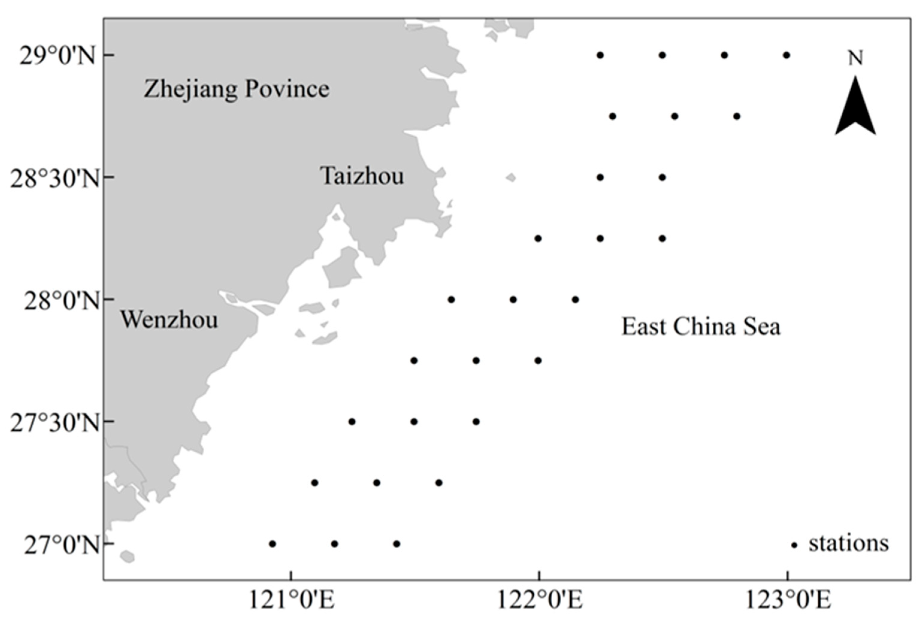
2.1. Data Sources

Decapterus maruadsi samples were collected from the offshore waters of southern Zhejiang and its adjacent waters (120.93° E–122.95° E, 27.21° N–28.97° N), and fishery resources and hydrographic surveys were conducted in May (spring), August (summer), November (autumn) and February (winter) from 2015 to 2020 (Figure 1). The survey gear is a bottom trawl with a total length of 95 m. The fishing gear is 40 m wide and 7.5 m high. The length of the ground rope and float line is 80 m. The mesh size of the net capsule is 2 cm, and the towing speed was 2–4 kn. At each survey station, environmental data such as water temperature and salinity were collected simultaneously using a WTW-Multi 3430 water analyzer. The collection, determination and analysis of water quality samples were carried out in accordance with the Specifications for Oceanographic Survey (GB/T 12763) [25] and Specification for Marine Monitoring (GB 17378) [26]. The survey data were standardized to a trawl speed of 3 kn and trawl time of 1 h before data analysis. The number of catches per unit time (N/h) was used as the density. As D. maruadsi were not caught in winter, only survey data from spring, summer and autumn were used for modeling purposes.

2.2. Modeling Process

Tweedie-GAM, which is suitable for dealing with excess zero values of the dependent variable, was selected as the base model and modeled separately at two different approaches. The fitting effect and predictive performance of the best model were compared under different approaches. The GAM, as a nonparametric regression method, can select different distribution families according to different data types to explore the relationship between fishery resources and environmental factors more accurately [11]. Since there are many zero values in D. maruadsi density data, this study uses the GAM following the Tweedie distribution to analyze them. The distribution is usually represented by T w p ( θ , φ ) and is fully determined by the variance function V ( μ ) = μ p , where θ is the norm parameter, φ is the dispersion parameter and p is the energy efficiency parameter. When p = 0, 1, 2 or 3, this corresponds to the Gaussian, Poisson, gamma or inverse Gaussian distributions, respectively. The distribution is a compound Poisson–gamma distribution when the value of p is between 1 and 2 [27], which is suitable for dealing with nonnegative data with a large number of zero values [28].

2.2.1. Selection of Explanatory Variables

Given that D. maruadsi performs seasonal migrations, such as spawning, overwintering and wintering migrations, there are spatial distribution differences in different seasons [20]. Moreover, D. maruadsi is a pelagic fish, and water temperature, salinity and depth are closely related to its distribution [3,21]. Therefore, season, surface water temperature, surface salinity, water depth, offshore distance, longitude and latitude were selected to explore the relationship between the distribution of D. maruadsi and environmental influencing factors. Offshore distance is the shortest distance from the survey station to the shore, which was calculated in the Sp package in R [29].
Before modeling, the variance inflation factor (VIF) test was performed to exclude highly correlated explanatory variables to prevent covariance from affecting the accuracy of the model [14]. It is generally believed that the problem of multicollinearity exists when VIF > 10 [16,30]. In addition, since this study focused on exploring the impact of modeling accuracy at different approaches, we used “season” as a categorical variable and did not test for covariance when building the Yearly-GAM.

2.2.2. Tweedie-GAM Development

In this study, Tweedie-GAM is used to establish the relationship between the density of D. maruadsi and environmental factors at two approaches, where the full factor expression of Yearly-GAM is:
g ( density ) = s e a s o n + s ( L a t ) + s ( L o n ) + s ( d e p t h ) + s ( D i s ) + s ( T ) + s ( S )
The full factorial expression for the subseasons GAM is:
g ( density ) = s ( L a t ) + s ( L o n ) + s ( d e p t h ) + s ( D i s ) + s ( T ) + s ( S )
where Lat denotes latitude; Lon denotes longitude; T denotes water temperature; S denotes salinity; depth denotes water depth; Dis denotes offshore distance; density denotes D. maruadsi density; and g is the link function.

2.2.3. Model Selection

The environmental factors after the covariance test were arranged and combined to build multiple Tweedie-GAMs between the density of D. maruadsi and the environmental factors. The goodness of fit of each model was measured by the Akaike information criterion (AIC) [31], and the best model was determined for both modeling approaches. The smaller the AIC value is, the better the fit of the model. In the later section, the best model for spring is Spring-GAM, the best model for summer is Summer-GAM, and the best model for autumn is Autumn-GAM. The AIC is calculated as follows:
AIC = 2 k 2 ln L
where k is the number of parameters and L is the likelihood function.

2.2.4. Model Evaluation

In this study, when comparing and evaluating the fitting effectiveness as well as the predictive performance of the two modeling approaches, the following three main aspects were evaluated.
(1)
Cross-validation. The predictive performance of the different models was compared by randomly selecting 80% of the data as the training set and the remaining 20% as the test set and running it 1000 times. For each cross-validation, a linear regression model was used to construct a linear relationship between the predicted and observed values, and the root mean square error (RMSE) and mean absolute error (MAE) between the predicted and observed values, as well as the mean of the coefficient of determination (R2), were calculated. When the RMSE and MAE are smaller and the R2 value is closer to 1, the model predicts better [32,33,34]. The regression equation is as follows:
ln Y = a + b × ln y
where y is the predicted value and Y is the observed value of the model. When a = 0 and b = 1, the predicted value and the observed value (i.e., test data) have a similar spatial pattern.
The equation for calculating the RMSE is as follows [32]:
R M S E = i = 1 n ( P i O i ) 2 n
The equation for calculating the MAE is [33]:
M A E = 1 n i = 1 n | ( P i O i ) |
where n is the number of observations, O i is the ith observed value, and P i is the ith predicted value.
(2)
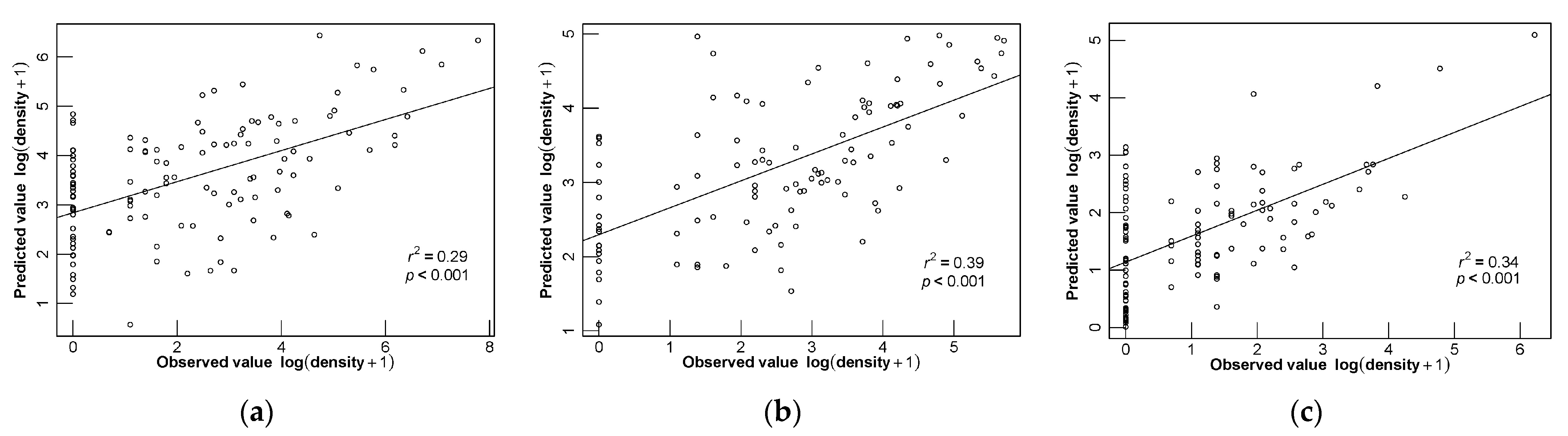
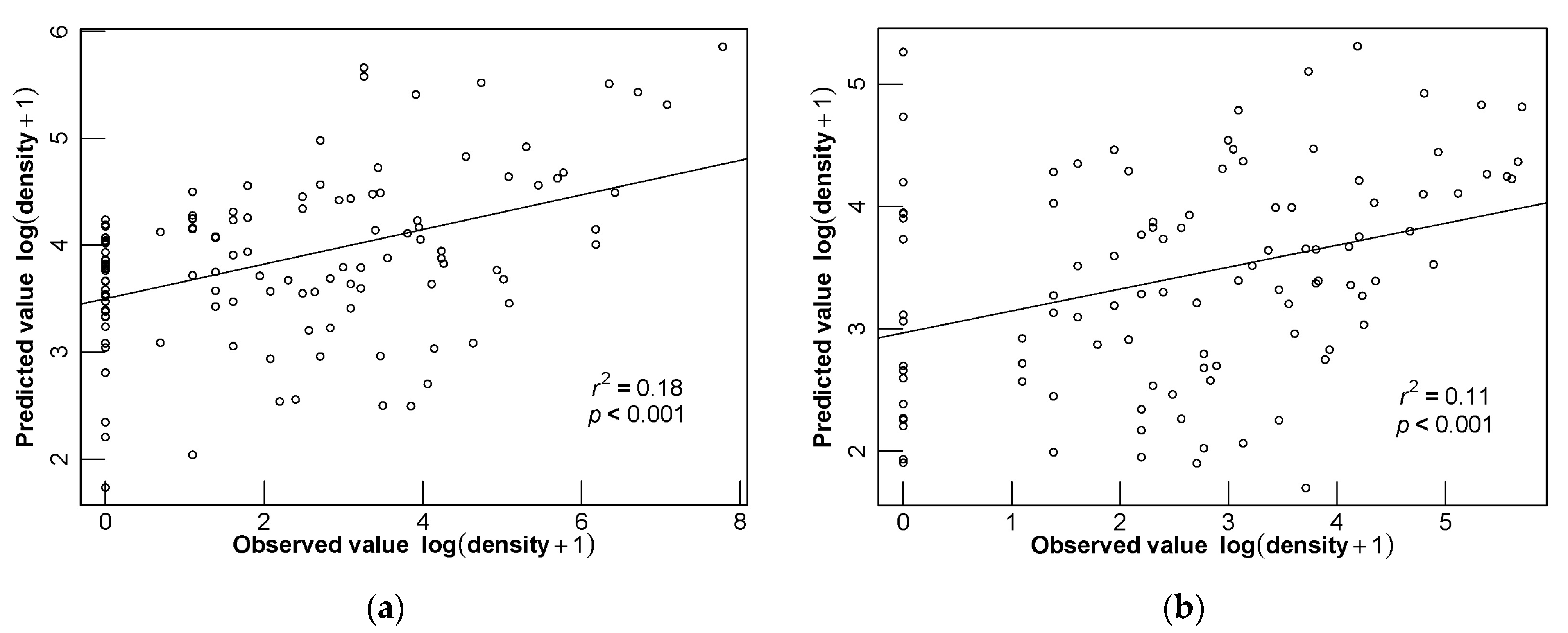
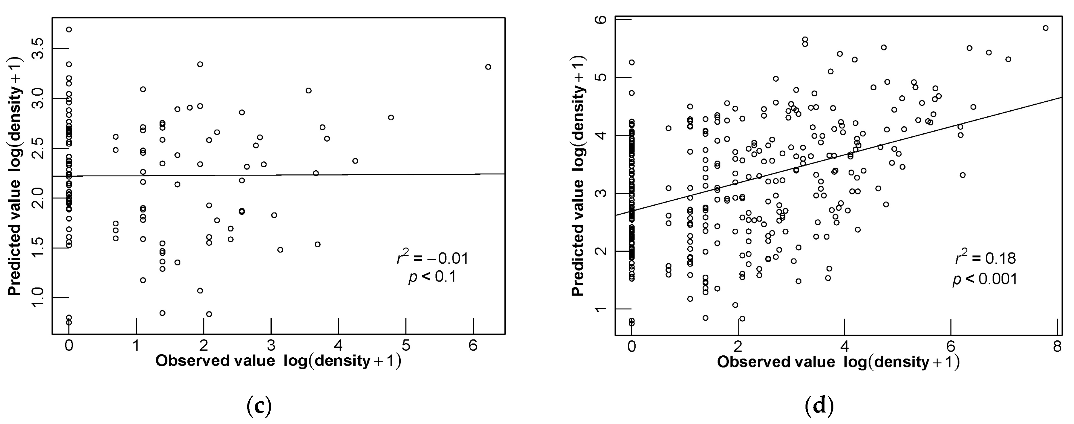
To evaluate the fitting effect between different models, this study used two different modeling approaches to predict the density of each station in each year and season and calculated the coefficient of determination (R2) and the significance (P) between the predicted and observed values.
(3)
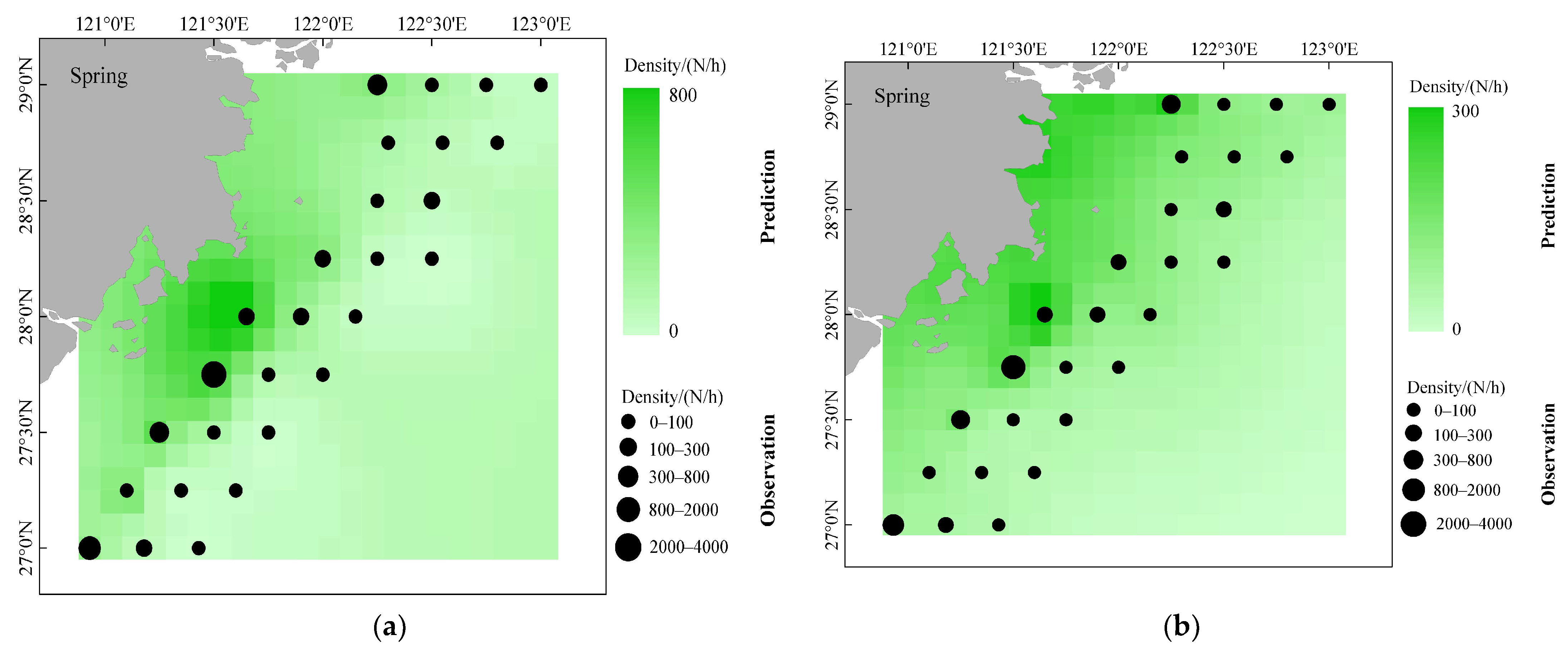
To assess the differences in the accuracy of predicting the spatial distribution of fishery resources by different modeling approaches, this study predicts the spatial distribution of D. maruadsi in different seasons by using two modeling approaches. A total of 420 quadrilateral grids were created for model prediction in the study area with a spatial resolution of 0.1° × 0.1°. The environmental factors in each grid were interpolated by using inverse distance weighting (IDW). The mean values of the observed and predicted values of D. maruadsi in different seasons from 2015 to 2020 were also superimposed and combined with the living habits of D. maruadsi to evaluate the prediction effects of the two modeling approaches.
All statistical analyses were performed in R software (V4.0.2). Tweedie-GAM was implemented using the “mgcv” package [35], and station and resource distribution maps were plotted in ArcMap 10.8.

3. Results

3.1. Collinearity Test

The collinearity test of the six predictor variables revealed that the VIF values of latitude and longitude in different seasons were greater than 10, while the VIF values of the other four predictor variables, such as salinity and offshore distance, were less than 10. After removing the longitude with the largest VIF value, the VIF values of latitude and other predictor variables were less than 10 (Table 1). In addition, the collinearity test was also performed for each predictor variable before establishing the Yearly-GAM, and it was also found that the VIF values of latitude and longitude were both greater than 10, and after removing the longitude with the largest VIF value, the VIF values of latitude and other predictor variables were all less than 10 (Table 1).

3.2. Optimal Model

In this study, models are built by arranging and combining the factors that do not covary. The energy efficiency parameters p in the Tweedie distribution were calculated to be 1.689, 1.534, 1.524 and 1.680 for different models, and the four models established follow a compound Poisson–gamma distribution (1 < p < 2).
The results of modeling by season are shown in Table 2. The best combination of variables in spring was water temperature, salinity and water depth, with a deviation explanation rate of 42.4%, while all three factors were significant influencing factors (p < 0.05). The best combination of variables in summer was water temperature, salinity, water depth and latitude, with a deviation explanation of 46.5%, and water temperature and latitude were significant influencing factors (p < 0.05). The best combination of variables in autumn was water temperature, salinity, depth and latitude, with a deviation explanation of 59% and salinity as a significant factor (p < 0.05). In contrast, in Yearly-GAM, the best combination of variables was season, water temperature, salinity, water depth and offshore distance, with 34.3% of the deviation explained.
The overall contribution explained by the factors that contributed the most (water temperature, water depth, season) varied across models being 20.0% in Summer-GAM, 35.8% in Summer-GAM, 24.6% in Autumn-GAM, and 13.2% in Yearly-GAM.

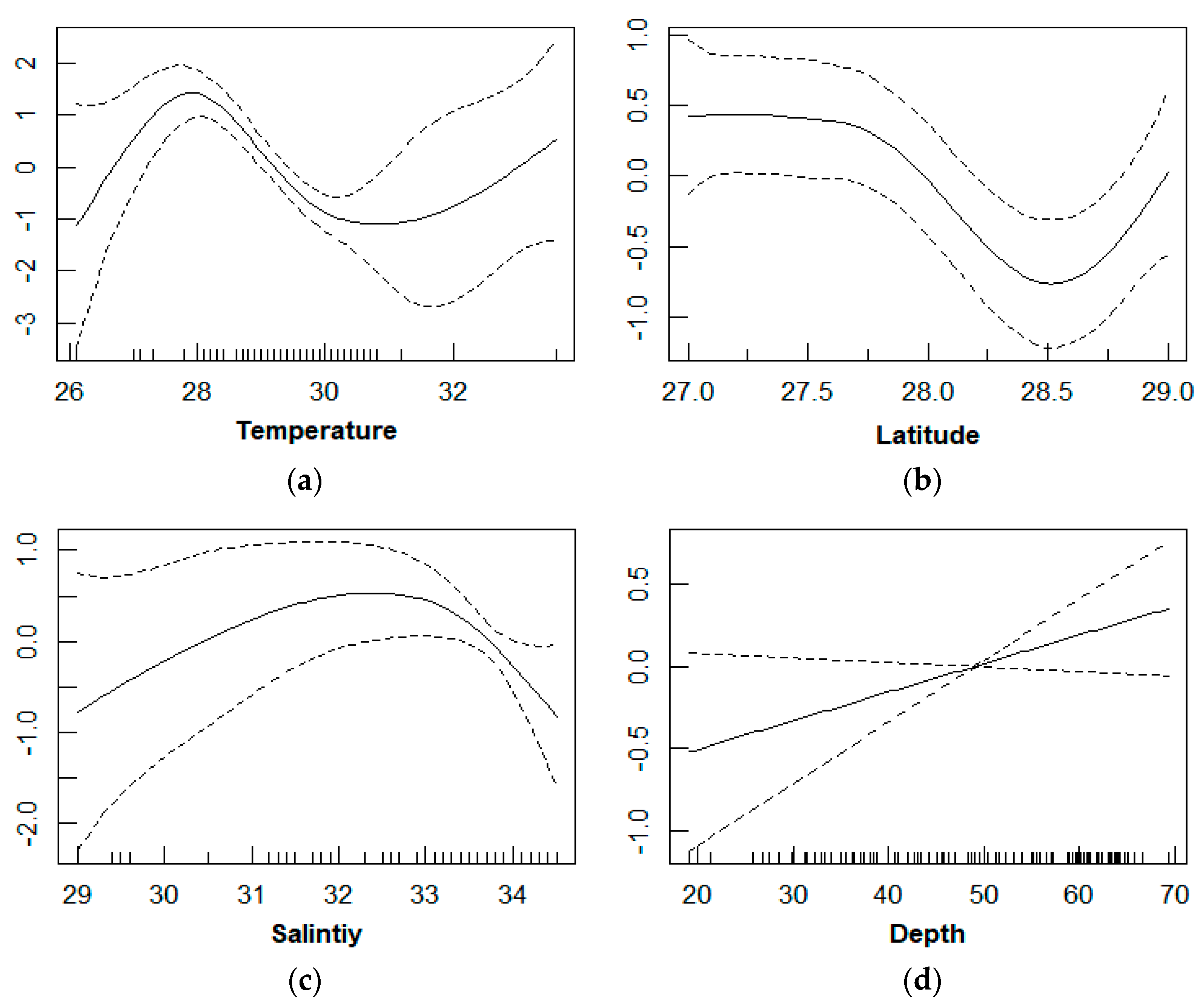
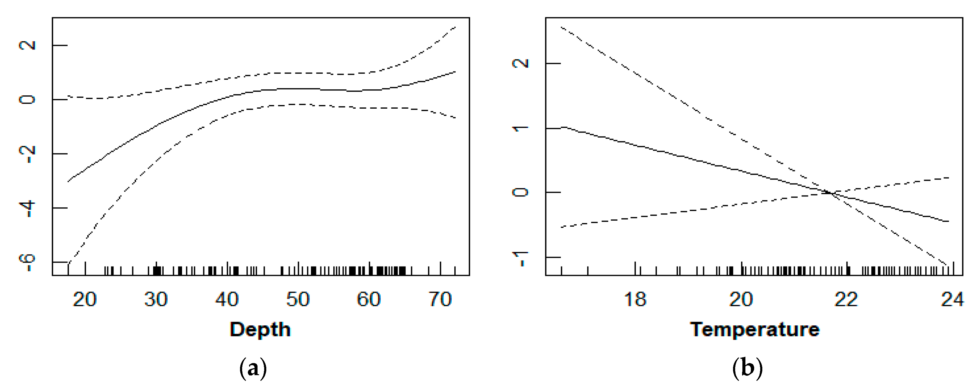
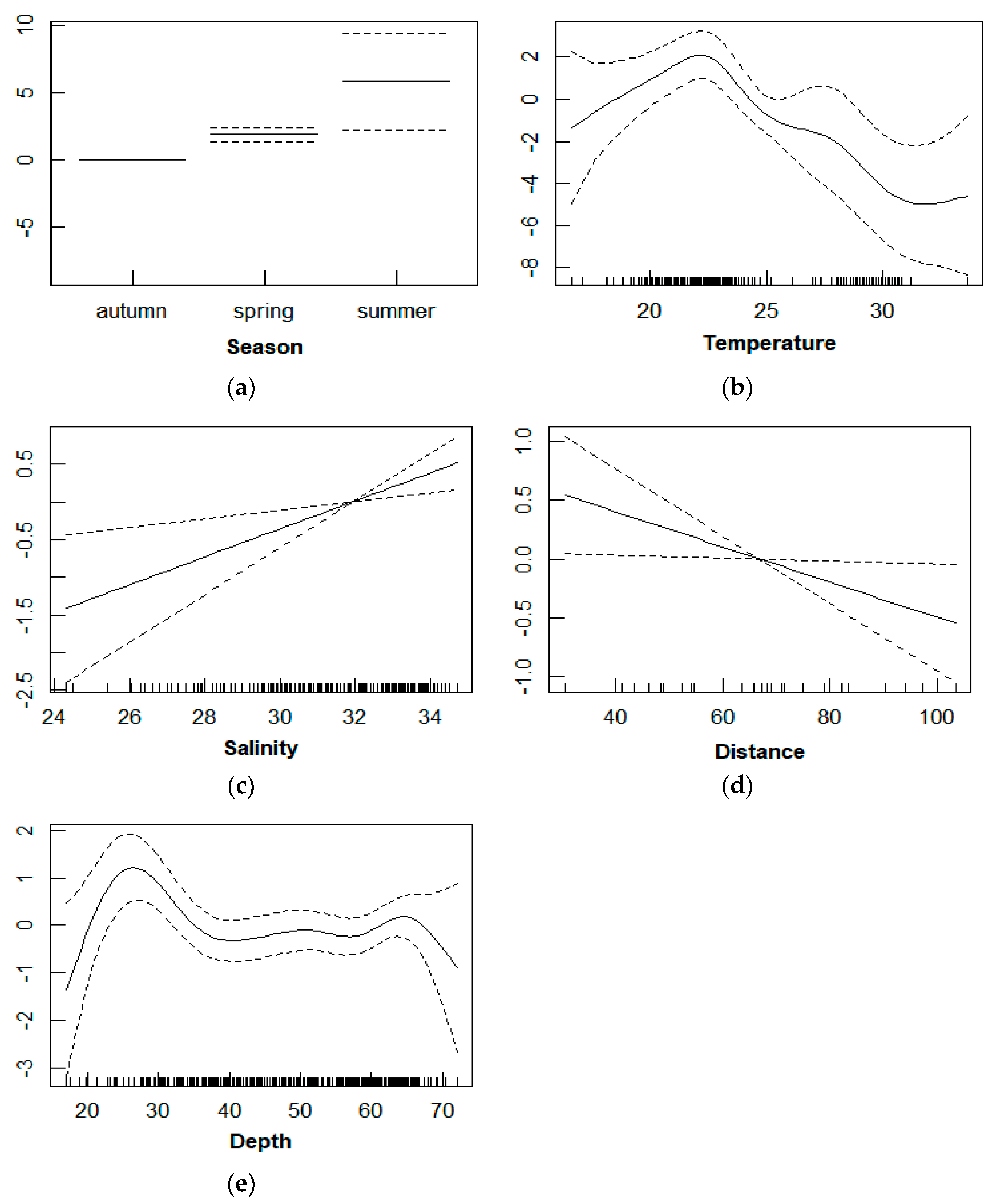
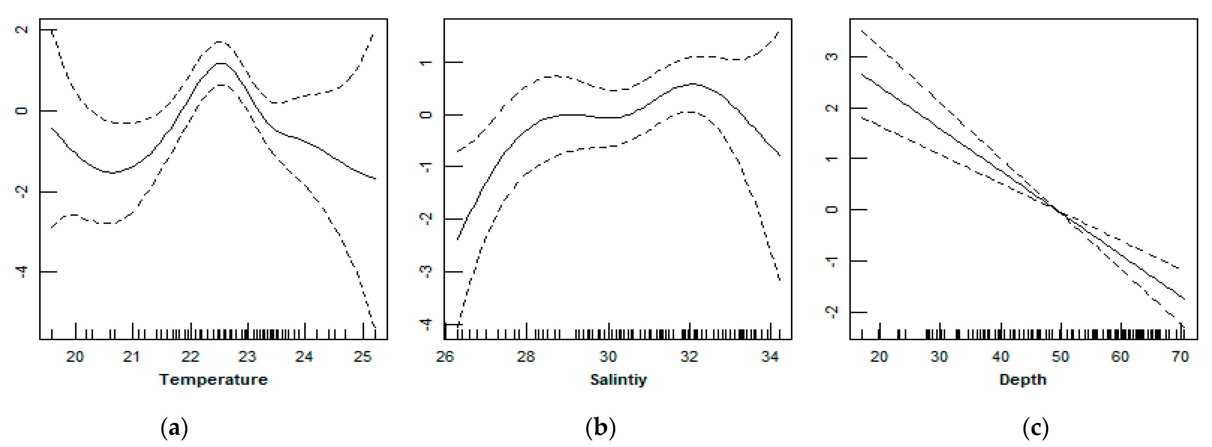
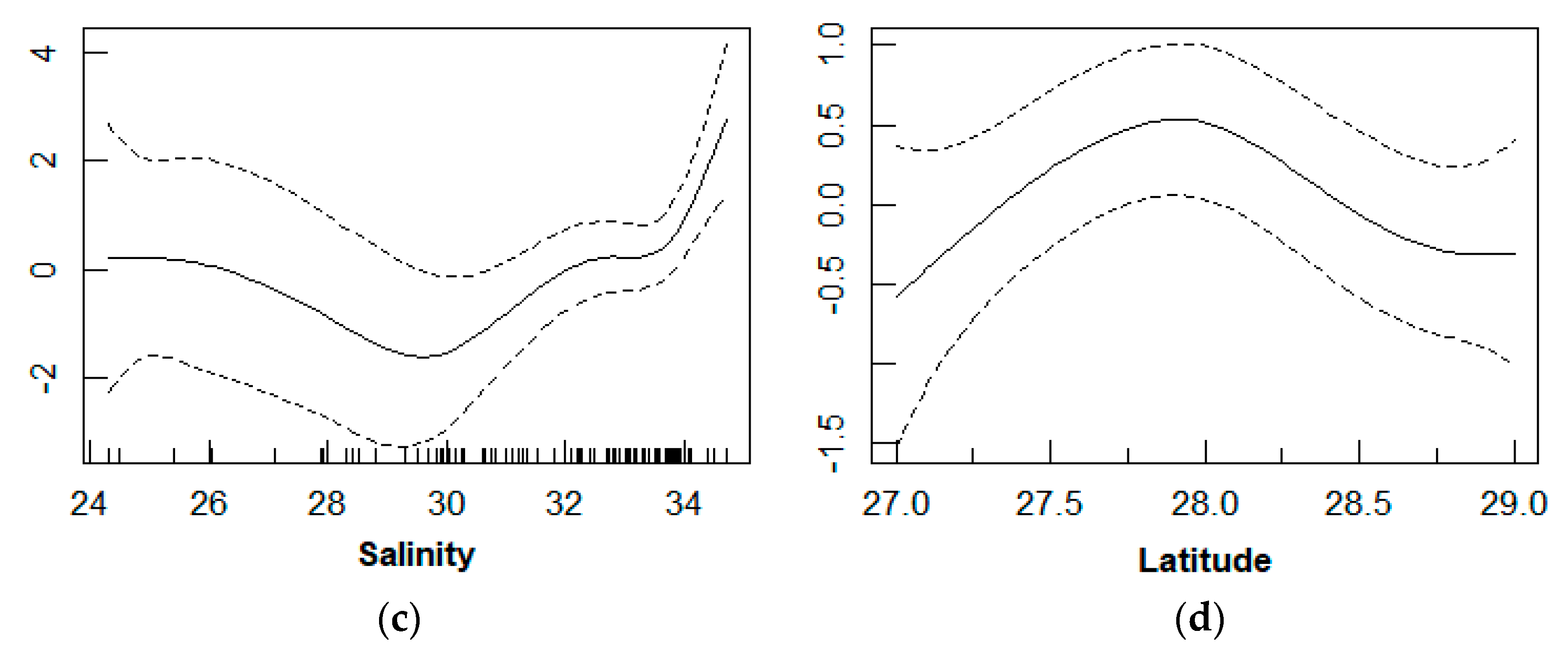
3.3. Relationship between D. maruadsi Density and Environmental Factors

Spring-GAM shows that in the water temperature range of 19.5–25 °C, the density shows an increasing and then a decreasing trend, the suitable temperature is 22–23 °C and density reaches a peak at 22.7 °C. In the salinity range from 26 to 34 ppt, the density showed an increasing and then a decreasing trend with increasing salinity and reached a maximum when the salinity was 32 ppt. There was a negative linear relationship between water depth and density, and the smaller the water depth was, the higher the density of D. maruadsi (Figure 2).
Summer-GAM showed that there was a multiwave nonlinear relationship between density and water temperature in the range of 26 °C–34 °C, showing an increasing trend, then a decreasing trend, followed by an increasing trend again, with peak and low density values obtained at 28 °C and 30.3 °C, respectively, and the suitable temperature range was 27 °C–29 °C. There is a single-peaked relationship between salinity and density; the suitable salinity range is 31.5–33 and density reaches the maximum when the salinity is 32.3. In the range of 20–70 m, there is a positive linear relationship between water depth and density, showing an increasing trend in density with increasing water depth (Figure 3).
Autumn-GAM shows that in the range of 20–70 m water depth, there is a nonlinear relationship between density and water depth, showing a general increasing trend first and then remaining basically the same, and the suitable water depth range is 35–70 m. In the range of 16–24 °C, the density gradually decreases with increasing water temperature. In the salinity range of 29–34.5 ppt, the density showed a decreasing and then an increasing trend with increasing salinity, and the suitable salinity range was 33–34 ppt (Figure 4).
There were obvious differences in the density of D. maruadsi in different seasons (Figure 5). Yearly-GAM showed that there was a peak-like relationship between water temperature and the density of D. maruadsi, showing an increasing and then a decreasing trend, and the maximum value was achieved at approximately 22 °C. There was a positive linear relationship between density and salinity, which gradually increased with increasing salinity. The relationship between the water depth and density of D. maruadsi showed an increasing and then a decreasing trend before leveling off, and the maximum value was achieved when the water depth was 27 m (Figure 5).

3.4. Model Evaluation

The cross-validation results showed that while the RMSE and MAE of Spring-GAM were larger than those of Yearly-GAM, the RMSE and MAE of Summer-GAM and Autumn-GAM were significantly smaller than those of Yearly-GAM, and the R2 of the three models built in different seasons was significantly higher than that of Yearly-GAM (Table 3). In addition, by comparing the observed and predicted values for different seasons and the whole year using different modeling approaches, we found that the goodness of fit of the model built by season was significantly higher than that of Yearly-GAM in different seasons (Figure 6 and Figure 7). Therefore, the model established by season can be considered a modeling method for predicting the density distribution of offshore D. maruadsi resources in southern Zhejiang, China, due to its reasonable fitting and relatively better predictability in mathematical statistics.

3.5. Different Seasonal Distributions of D. maruadsi and Predictive Performance of Different Models

In this study, by using the mean values of the D. maruadsi density in spring, summer and autumn from 2015 to 2020 to map its spatial distribution, it was found that D. maruadsi showed different distribution patterns in different seasons (Figure 2). Among them, the density in spring was significantly higher than that in summer and autumn. In spring, D. maruadsi was mainly distributed in inshore waters south of 28° N and 29° N. Compared with spring, D. maruadsi in summer was mainly concentrated in waters north of 28°45′ N and south of 27°45′ N. In autumn, the distribution pattern of D. maruadsi density was opposite to that of spring, showing the distribution characteristics that waters on the seaward side had a higher D. maruadsi density than inshore waters, with the resource mainly distributed in the outer waters at and north of 28° N (Figure 8). In this study, by comparing the predicted and observed values of the two modeling approaches, we found that although there are some differences between the predicted and observed values of these two types of models, the predictive performance of the model built by season is significantly higher than that of Yearly-GAM and closer to the real density (Figure 8). In addition, this study also found that, in Yearly-GAM, the predicted resource densities in all three seasons showed the distribution characteristics that inshore waters had a significantly higher D. maruadsi density than that in offshore waters, while in the model built by season, the three seasons showed different distribution characteristics.

4. Discussion

4.1. Model Comparison

Species distribution models are essential for predicting distributions and promoting species conservation because of the difficulty of monitoring species distributions over large spatial areas [8]. Predicted values obtained through modeling and simulation are considered an important goal of ecological and environmental research, as they can show whether decisions made by environmental managers are adequate and appropriate, and therefore need to be as accurate as possible [36]. In this study, two different modeling approaches were used to predict density as well as spatial distribution in different seasons. We evaluated the fitting effectiveness of these two approaches, as well as their predictive performance by cross-validation, and linked them to real-life habits. The results show that modeling by season has better predictive performance and that the model fits more accurately. Related studies have shown that when exploring the spatial distribution of resources, an effective understanding of the density and the combination of spatial distribution variables helps to further understand the physiological and behavioral characteristics of the target species [37]. Many scholars have suggested that the effects of different environmental factors in different seasons differ in degree [3,8,38]. Therefore, accurate knowledge of the weights of each factor when building a species distribution model will effectively increase the reliability and stability of the model. In this study, it was found that the model built by season by selecting the resource distribution characteristics in different seasons and their key influencing factors is more consistent with the actual distribution. However, in Yearly-GAM, the weights of each environmental factor and the relationship with density were found to be consistent across seasons (Table 2). This is contrary to the findings of Vayghan et al. [39] and differs significantly from the actual situation. The present study speculates that this may be because modeling with year-round data weakens the variability in density and predictor variables across seasons, thus limiting the model fit and predictive performance.

4.2. Spatial and Temporal Distribution of D. maruadsi Density

In this study, it was found that there were seasonal variations in the density and spatial distribution of D. maruadsi offshore of southern Zhejiang. Compared with summer and autumn, the highest density was found in spring (Figure 7), which may be due to the phenomenon of seawater rising from the bottom to compensate for the action of the southwest monsoon in spring off southern Zhejiang, which easily formed the area with higher chlorophyll a content [40,41]. This makes plankton reproduction flourish, thus providing food for D. maruadsi or other D. maruadsi bait organisms, making the density of D. maruadsi richer in this sea area. In addition, spring is the spawning season of D. maruadsi [42], and because the physical structure of inshore waters is relatively complex [43], it can promote the coexistence of various organisms and thus provide more bait organisms for D. maruadsi juveniles and parents. Thus, D. maruadsi are mainly concentrated in inshore waters in spring, which shows that this resource’s density in inshore waters is significantly higher than that in offshore waters (Figure 7a,b). From July to October each year, D. maruadsi began to gradually move northward to feed on bait in northern Zhejiang, often gathering in patches [20], which may explain the phenomenon of higher density and clustering of D. maruadsi in southern Zhejiang waters in summer. From October to November each year, as the water temperature gradually decreases, D. maruadsi begin to gradually move southward into their wintering grounds [44], which makes this resource’s density in summer and autumn significantly lower than that in spring.
In the two types of models, the spatially predicted distribution trends of summer and autumn showed opposite patterns. In the subseasonal establishment model, the predicted spatial trend of D. maruadsi showed a greater density in offshore waters than in inshore waters, while in Yearly-GAM, the predicted spatial distribution characteristics showed a trend of greater density in inshore waters than in offshore waters. Related studies showed [42] that the D. maruadsi stock had a tendency to move gradually offshore for baiting in summer and autumn, so this study concluded that the predicted spatial distribution by seasonal modeling was more consistent with the actual situation. In addition, the present study also found that in spring, the predicted effect of Spring-GAM was closer to the real density than that of Yearly-GAM. Meanwhile, the actual resource distribution characteristics of the surveyed sites in this study will also be more accurately modeled by season compared with the predicted resource distribution characteristics (Figure 7 and Figure 8). Therefore, this study compared the spatial distribution characteristics of D. maruadsi and the absolute density offshore of southern Zhejiang Province and concluded that the prediction effect of the model built by seasons was better than that of Yearly-GAM.

4.3. Relationship between D. maruadsi Density and Environmental Factors

In this study, water depth was the environmental factor with the largest deviation explanation rate in Spring-GAM and Autumn-GAM, and water temperature was the environmental factor with the largest deviation explanation rate in Summer-GAM, while water temperature, salinity and water depth appeared in all models. Thus, this study concluded that water temperature, salinity and water depth were the important influencing factors affecting the distribution of D. maruadsi resources offshore of southern Zhejiang, China.
Water temperature is one of the important environmental factors affecting all fish growth stages and can influence not only fish growth and development and spawning migration [45] but also fish distribution and migration indirectly by changing the spatial and temporal distribution of bait and density [46]. In this study, the relationship between D. maruadsi density and water temperature differed significantly among the four models. However, in both Spring-GAM and Yearly-GAM, the relationship between density and water temperature was generally consistent, and the peak density was achieved at 22.4 °C. This study suggests that the reason for this might be that the density in spring is significantly higher than that in summer and autumn, which makes the relationship between density and water temperature of D. maruadsi in spring more prominent in the fitting process of the model, thus producing a high agreement between the two factors. In addition, this study also found that the suitable temperature range for D. maruadsi in the spring was 22–23 °C and 27–29 °C in summer in the offshore waters of southern Zhejiang. However, compared with other waters, the suitable water temperature of D. maruadsi in different seasons had significant geographical differences. Zhao et al. [3] found that the suitable spring temperature range of D. maruadsi in northern South China Sea waters was 24.4–26.8 °C, and He et al. [42] found that the suitable temperature range of D. maruadsi in the northwestern South China Sea was 25–26 °C in spring and 29–30 °C in summer. In addition, Fan et al. [47] found that the summer temperature range of D. maruadsi in the northern waters of the South China Sea was 29–29.7 °C. This study suggests that this significant geographical difference may be related to the fact that the water temperature in the southern Zhejiang waters may also be lower than that in the South China Sea during the same period. In addition, there are also differences in D. maruadsi populations in different waters [44,48], which may result in different adaptation ranges to water temperature.
Salinity plays an important role in fish growth and development, affecting fish metabolism and survival of eggs and juveniles through osmolarity [3,8], and is also a key influence on the spatial and temporal distribution structure of fish [45]. Zhu et al. [49] showed that juvenile D. maruadsi are usually found in mixed saltwater and freshwater areas, and adults tend to be found in the frontier of high salinity water. This study found that there was some variation in salinity in the relationship between density and salinity in the four models established. However, there was a common feature in all four models that high D. maruadsi density values were found in waters with higher salinity. This is generally consistent with the findings of He et al. [42] that high D. maruadsi density values in the northwestern South China Sea occur in waters with salinities of 33.4 to 33.8 ppt and that fishing grounds for juvenile and adult D. maruadsi in the East China Sea are usually located in high salinity waters [49].
Water depth, as a comprehensive influencing factor, can not only directly reflect changes in pressure and light intensity but also indirectly reflect changes in environmental conditions such as water temperature and salinity [9,50]. Related studies have shown [42] that D. maruadsi are mainly concentrated in inshore waters in spring for spawning and baiting, while in summer and autumn, they are mainly adult fish, which are more adaptable to the environment and can enter deeper waters for baiting and feeding. In the present study, the seasonal model also showed that D. maruadsi was concentrated in shallow waters in spring and in deeper waters in summer and autumn (Figure 2, Figure 3 and Figure 4). However, in the Yearly-GAM, the density showed an increasing then decreasing trend, and then stabilized, and reached a maximum at 27 m (Figure 5), which is different from the results of the seasonal modeling and the actual situation. This may be because the living habits of D. maruadsi vary significantly in different seasons [3,42], whereas Yearly-GAM is modeled with year-round data, which to a certain extent weakens the differences in living habits of D. maruadsi in different seasons.
In this study, Tweedie-GAM was used to predict the spatial distribution of D. maruadsi in different seasons as well as the absolute density to compare the model prediction accuracy of the two modeling approaches. Although there were some differences between the predicted density of D. maruadsi and the true density in this study using GAM, it was sufficient for comparing the fitting effect and predictive performance of the two types of models. However, this study finds that the predictive performance of the model in different seasons is not very good (Table 3) and speculates that this may be caused by the small amount of data with many zero values. In addition, related studies have shown that the spatial distribution of target species can also be inferred indirectly using biological factors (e.g., bait organisms) [8] and interactions between organisms (e.g., predation) [51]. Therefore, biological factors will be incorporated in future studies, and more marine environmental factors will be collected to improve the accuracy and prediction of the models.

5. Conclusions

This study is based on independent survey data of offshore fishery resources and hydrographic environment data from 2015–2020 in southern Zhejiang, China, and used Tweedie-GAM as the base model. The effects of two different approaches to seasons on the predictive performance of the species distribution model were compared. The results showed that the modeling by season had better fitting and predictive performance compared to Yearly-GAM. It is also more accurate in exploring the relationship between target species density and environmental factors. In terms of the spatial distribution of fishery resources, the spatial distribution predicted by Yearly-GAM has similar spatial distribution, i.e., they all show the distribution characteristics that the density of inshore waters is greater than that of offshore waters. However, in the model established by season, different seasons show different distribution patterns, which are more consistent with the actual spatial distribution.

Author Contributions

Data analysis was performed by W.M. and J.Z.; W.M. wrote the first draft of the manuscript; S.Q., C.G. and J.M. designed the survey; J.Z. revised the manuscript and approved it for submission. All authors have read and agreed to the published version of the manuscript.

Funding

This research was funded by the National Natural Science Foundation of China (31902372) and the Fisheries Resource Survey of Zhejiang Province, China (158053).

Institutional Review Board Statement

Not applicable.

Informed Consent Statement

Not applicable.

Data Availability Statement

Data is contained within the article.

Acknowledgments

The authors of this research would like to thank the teachers and students from the Research Laboratory of Quantitative Assessment and Management of Fisheries Resources and Ecosystems, Shanghai Ocean University and Zhejiang Mariculture Research Institute.

Conflicts of Interest

The authors declare no conflict of interest.

References

  1. Zhao, J.; Cao, J.; Tian, S.; Chen, Y.; Zhang, S.; Wang, Z.; Zhou, X. A comparison between two GAM models in quantifying relationships of environmental variables with fish richness and diversity indices. Aquat. Ecol. 2014, 48, 297–312. [Google Scholar] [CrossRef]
  2. Long, X.Y.; Wan, R.; Li, Z.G.; Ren, Y.P.; Song, P.B.; Tian, Y.J.; Xu, B.D.; Xue, Y. Spatio-temporal distribution of Konosirus punctatus spawning and nursing ground in the South Yellow Sea. Acta Oceanol. Sin. 2021, 40, 133–144. [Google Scholar] [CrossRef]
  3. Zhao, H.; Feng, Y.T.; Dong, C.M.; Li, Z.L. Spatiotemporal distribution of Decapterus maruadsi in spring and autumn in response to environmental variation in the northern South China Sea. Reg. Stud. Mar. Sci. 2021, 45, 101811. [Google Scholar] [CrossRef]
  4. Pan, S.Y.; Tian, S.Q.; Wang, X.F.; Dai, L.B.; Gao, C.X.; Tong, J.F. Comparing different spatial interpolation methods to predict the distribution of fishes: A case study of Coilia nasus in the Changjiang River Estuary. Acta Oceanol. Sin. 2021, 40, 119–132. [Google Scholar] [CrossRef]
  5. Tian, S.Q.; Chen, X.J.; Chen, Y.; Xu, L.X.; Dai, X.J. Evaluating habitat suitability indices derived from CPUE and fishing effort data for Ommatrephes bratramii in the northwestern Pacific Ocean. Fish. Res. 2009, 95, 181–188. [Google Scholar] [CrossRef]
  6. Zhang, Y.L.; Zhang, C.L.; Xu, B.D.; Ji, Y.P.; Ren, Y.P.; Xue, Y. Impacts of trophic interactions on the prediction of spatio-temporal distribution of mid-trophic level fishes. Ecol. Indic. 2022, 138, 108826. [Google Scholar] [CrossRef]
  7. Yu, H.; Cooper, A.R.; Infante, D.M. Improving species distribution model predictive accuracy using species abundance: Application with boosted regression trees. Ecol. Model. 2020, 432, 109202. [Google Scholar] [CrossRef]
  8. Liu, X.X.; Wang, J.; Zhang, Y.L.; Yu, H.M.; Xu, B.D.; Zhang, C.L.; Ren, Y.P.; Xue, Y. Comparison between two GAMs in quantifying the spatial distribution of Hexagrammos otakii in Haizhou Bay, China. Fish. Res. 2019, 218, 209–217. [Google Scholar] [CrossRef]
  9. Liu, X.X.; Gao, C.X.; Zhao, J.; Tian, S.Q.; Ye, S.; Ma, J. Modeling and comparison of count data containing zero values: A case study of Setipinna taty in the south inshore of Zhejiang, China. Environ. Sci. Pollut. Res. 2021, 28, 46827–46837. [Google Scholar] [CrossRef]
  10. Elith, J.H.; Graham, C.P.; Anderson, R.; Dudík, M.; Ferrier, S.; Guisan, A.J.; Hijmans, R.; Huettmann, F.R.; Leathwick, J.; Lehmann, A. Novel methods improve prediction of species’ distributions from occurrence data. Ecography 2006, 29, 129–151. [Google Scholar] [CrossRef] [Green Version]
  11. Luan, J.; Zhang, C.L.; Ji, Y.P.; Xu, B.D.; Xue, Y.; Ren, Y.P. Matching data types to the objectives of species distribution modeling: An evaluation with marine fish species. Front. Mar. Sci. 2021. [Google Scholar] [CrossRef]
  12. Meng, W.Z.; Gong, Y.H.; Wang, X.F.; Tong, J.F.; Han, D.Y.; Chen, J.H.; Wu, J.H. Influence of spatial scale selection of environmental factors on the prediction of distribution of Coilia nasus in Changjiang River Estuary. Fishes 2021, 6, 48. [Google Scholar] [CrossRef]
  13. Bouska, K.L.; Whitledge, G.W.; Lant, C. Development and evaluation of species distribution models for fourteen native central U.S. fish species. Hydrobiologia 2015, 747, 159–176. [Google Scholar] [CrossRef]
  14. Dai, L.B.; Hodgdon, C.; Tian, S.Q.; Chen, J.H.; Gao, C.X.; Han, D.Y.; Kindong, R.; Ma, Q.Y.; Wang, X.F. Comparative performance of modelling approaches for predicting fish species richness in the Yangtze River Estuary. Reg. Stud. Mar. Sci. 2020, 35, 101161. [Google Scholar] [CrossRef]
  15. Chang, J.H.; Chen, Y.; Holland, D.; Grabowski, J. Estimating spatial distribution of American lobster Homarus americanus using habitat variables. Mar. Ecol. Prog. Ser. 2010, 420, 145–156. [Google Scholar] [CrossRef]
  16. Hua, C.X.; Zhu, Q.C.; Shi, Y.C.; Liu, Y. Comparative analysis of CPUE standardization of Chinese Pacific saury (Cololabis saira) fishery based on GLM and GAM. Acta Oceanol. Sin. 2019, 38, 100–110. [Google Scholar] [CrossRef]
  17. Bellido, J.M.; Pierce, G.J.; Wang, J. Modelling intra-annual variation in abundance of squid Loligo forbesi in Scottish waters using generalised additive models. Fish. Res. 2001, 52, 23–39. [Google Scholar] [CrossRef]
  18. Shono, H. Application of the Tweedie distribution to zero-catch data in CPUE analysis. Fish. Res. 2008, 93, 154–162. [Google Scholar] [CrossRef] [Green Version]
  19. Zhang, T.J.; Song, L.M.; Yuan, H.C.; Song, B.; Ebango Ngando, N. A comparative study on habitat models for adult bigeye tuna in the Indian Ocean based on gridded tuna longline fishery data. Fish. Oceanogr. 2021, 30, 584–607. [Google Scholar] [CrossRef]
  20. Zhang, Q.H.; Cheng, J.H.; Xu, H.X.; Shen, X.Q.; Yu, G.P.; Zheng, Y.J. Fishery Resources and Their Sustainable Utilization in the East China Sea; Fudan University: Shanghai, China, 2007. [Google Scholar]
  21. Yu, J.; Liu, Z.N.; Chen, P.M.; Yao, L.J. Environmental factors affecting the spatiotemporal distribution of Decapterus maruadsi in the western Guangdong waters, China. Appl. Ecol. Env. Res. 2019, 17, 8485–8499. [Google Scholar] [CrossRef]
  22. Jiang, R.J.; Xu, H.X.; Jin, H.W.; Zhou, Y.D.; He, Z.T. Feeding habits of blue mackerel scad Decapterus maruadsi Temminck et Schlegel in the East China Sea. J. Fish. China 2012, 36, 216–227. [Google Scholar]
  23. Xu, W.; Yang, R.; Chen, G.; Gao, C.X.; Ye, S.; Han, D.Y. Feeding ecology of Decapterus maruadsi in the southern coastal area of Zhejiang based on stomach contents and stable isotope analysis. J. Appl. Ecol. 2022, 1–10. [Google Scholar] [CrossRef]
  24. Cui, M.Y.; Chen, W.F.; Dai, L.B.; Ma, Q.Y. Growth heterogeneity and natural mortality of Japanese scad in offshore waters of southern Zhejiang. J. Fish. Sci. China 2020, 27, 1427–1437. [Google Scholar]
  25. General Administration of Quality Supervision, Inspection and Quarantine of the People’s Republic of China, Standardization Administration of the People’s Republic of China. National Standard (Recommended) of the People’s Republic of China: Specifications for Oceanographic Survey—Part 6: Marine Biological Survey, GB/T 12763.6–2007; Standards Press of China: Beijing, China, 2008.
  26. General Administration of Quality Supervision, Inspection and Quarantine of the People’s Republic of China. GB17378.3–2007 the Specification for Marine Monitoring—Part 3: Sample Collection, Storage and Transportation; China Standards Press: Beijing, China, 2008.
  27. Tanaka, K.R.; Chang, J.H.; Xue, Y.; Li, Z.G.; Jacobson, L.; Chen, Y. Mesoscale climatic impacts on the distribution of Homarus americanus in the US inshore Gulf of Maine. Can. J. Fish. Aquat. Sci. 2019, 76, 608–625. [Google Scholar] [CrossRef] [Green Version]
  28. Berg, C.W.; Nielsen, A.; Kristensen, K. Evaluation of alternative age–based methods for estimating relative abundance from survey data in relation to assessment models. Fish. Res. 2014, 151, 91–99. [Google Scholar] [CrossRef]
  29. Pebesma, E.; Bivand, R.S. S classes and methods for spatial data: The sp package. R News 2005, 5, 9–13. [Google Scholar]
  30. Bui, D.T.; Lofman, O.; Revhaug, I.; Dick, O. Landslide susceptibility analysis in the Hoa Binh province of Vietnam using statistical index and logistic regression. Nat. Hazards 2011, 59, 1413–1444. [Google Scholar] [CrossRef]
  31. Planque, B.; Bellier, E.; Lazure, P. Modelling potential spawning habitat of sardine (Sardina pilchardus) and anchovy (Engraulis encrasicolus) in the Bay of Biscay. Fish. Oceanogr. 2007, 16, 16–30. [Google Scholar] [CrossRef]
  32. Stow, C.A.; Jolliff, J.; McGillicuddy, D.J.; Doney, S.C.; Allen, J.I.; Friedrichs, M.A.M.; Rose, K.A.; Wallhead, P. Skill assessment for coupled biological/physical models of marine systems. J. Mar. Syst. 2009, 76, 4–15. [Google Scholar] [CrossRef] [Green Version]
  33. Willmott, C.J.; Matsuura, K. Advantages of the mean absolute error (MAE) over the root mean square error (RMSE) in assessing average model performance. Clim. Res. 2005, 30, 79–82. [Google Scholar] [CrossRef]
  34. Ma, W.; Gao, C.X.; Tang, W.; Qin, S.; Ma, J.; Zhao, J. Relationship between Engraulis japonicus resources and environmental factors based on multi-model comparison in offshore waters of southern Zhejiang, China. J. Mar. Sci. Eng. 2022, 10, 657. [Google Scholar] [CrossRef]
  35. Wood, S.N.; Pya, N.; Säfken, B. Smoothing parameter and model selection for general smooth models. J. Am. Stat. Assoc. 2016, 111, 1548–1563. [Google Scholar] [CrossRef]
  36. Franca, S.; Cabral, H.N. Predicting fish species richness in estuaries: Which modelling technique to use? Environ. Model. Softw. 2015, 66, 17–26. [Google Scholar] [CrossRef]
  37. Zeng, Y.; Yeo, D.C.J. Assessing the aggregated risk of invasive crayfish and climate change to freshwater crabs: A Southeast Asian case study. Biol. Conserv. 2018, 223, 58–67. [Google Scholar] [CrossRef]
  38. Zhang, Y.L.; Yu, H.M.; Yu, H.Q.; Xu, B.D.; Zhang, C.L.; Ren, Y.P.; Xue, Y.; Xu, L.L. Optimization of environmental variables in habitat suitability modeling for mantis shrimp Oratosquilla oratoria in the Haizhou Bay and adjacent waters. Acta Oceanol. Sin. 2020, 39, 36–47. [Google Scholar] [CrossRef]
  39. Valavanis, V.D.; Georgakarakos, S.; Kapantagakis, A.; Palialexis, A.; Katara, I. A GIS environmental modelling approach to essential fish habitat designation. Ecol. Model. 2004, 178, 417–427. [Google Scholar] [CrossRef]
  40. Zhang, C.; Shang, S.; Hong, H. Spatial patterns of annual cycles in surface chlorophyll a in the Taiwan Strait. Acta Oceanol. Sin. 2006, 28, 165–170. [Google Scholar]
  41. Liu, X.X.; Gao, C.X.; Tian, S.Q.; Qin, S.; Ma, J.; Zhao, J. Distribution of Setipinna taty optimal habitats in the South inshore area of Zhejiang Province based on the habitat suitability index. J. Fish. Sci. China 2020, 27, 1485–1495. [Google Scholar]
  42. He, L.X.; Fu, D.Y.; Li, Z.L.; Wang, H.; Sun, Y.; Liu, B.; Yu, G. Spatio–temporal distribution of Decapterus maruadsi and its relationship with environmental factors in the northwestern South China Sea. Prog. Fish. Sci. 2022, 1–12. [Google Scholar] [CrossRef]
  43. Chen, W.F.; Peng, X.; Wang, Z.H.; Xie, Q.L.; Chen, S.B.; Ye, S.; Chen, Y.; Ai, W.M. Community structure characteristics of fishes in the coastal area of south Zhejiang during autumn and winter. Ocean Dev. Manag. 2017, 34, 111–119. [Google Scholar]
  44. Zheng, Y.J.; Li, J.S.; Zhang, Q.Y.; Hong, W.S. Research progresses of resource biology of important marine pelagic food fishes in China. J. Fish. China 2014, 38, 149–160. [Google Scholar]
  45. Kindong, R.; Chen, J.H.; Dai, L.B.; Gao, C.X.; Han, D.Y.; Tian, S.Q.; Wu, J.H.; Ma, Q.Y.; Tang, J.Y. The effect of environmental conditions on seasonal and inter–annual abundance of two species in the Yangtze River estuary. Mar. Freshw. Res. 2021, 72, 493–506. [Google Scholar] [CrossRef]
  46. Lewin, W.C.; Mehner, T.; Ritterbusch, D.; Brämick, U. The influence of anthropogenic shoreline changes on the littoral abundance of fish species in German lowland lakes varying in depth as determined by boosted regression trees. Hydrobiologia 2014, 724, 293–306. [Google Scholar] [CrossRef]
  47. Fan, J.T.; Huang, Z.R.; Xu, Y.W.; Sun, M.S.; Chen, G.B.; Chen, Z.Z. Habitat model analysis for Decapterus maruadsi in northern south China sea based on remote sensing data. Trans. Oceanol. Limnol. 2018, 3, 142–147. [Google Scholar]
  48. Niu, S.F.; Wu, R.X.; Zhai, Y.; Zhang, H.R.; Li, Z.L.; Liang, Z.B.; Chen, Y.H. Demographic history and population genetic analysis of Decapterus maruadsi from the northern South China Sea based on mitochondrial control region sequence. PeerJ 2019, 7, e7953. [Google Scholar] [CrossRef] [Green Version]
  49. Zhu, D.L.; Song, H.T.; Bo, Z.L.; Wu, Z.J. A study on mackerel and round scad fishing ground off Zhejiang coast in the summer–autumn season. Mar. Sci. Bull. 1984, 2, 62–70. [Google Scholar]
  50. Feng, Y.T.; Shi, H.Y.; Hou, G.; Zhao, H.; Dong, C.M. Relationships between environmental variables and spatial and temporal distribution of jack mackerel (Trachurus japonicus) in the Beibu Gulf, South China Sea. PeerJ 2021, 9, e12337. [Google Scholar] [CrossRef]
  51. Yalcin, E.; Gurbet, R. Environmental Influences on the spatio–temporal distribution of European Hake (Merluccius merluccius) in Izmir Bay, Aegean Sea. Turk. J. Fish. Aquat. Sci. 2016, 16, 1–14. [Google Scholar] [CrossRef]
Figure 1. Sampling stations for the distribution of fish resources and hydrological environment sampling stations in offshore waters south of Zhejiang.
Fishes 07 00153 g001
Figure 2. Relationship between the density of D. maruadsi and environmental factors in coastal waters of southern Zhejiang at seasonal scales (Spring): (a) effect of temperature; (b) effect of salinity and (c) effect of depth. Dashed lines show 95% confidence intervals.
Fishes 07 00153 g002
Figure 3. Relationship between the density of D. maruadsi and environmental factors in coastal waters of southern Zhejiang at seasonal scales (Summer): (a) effect of temperature;(b) effect of latitude; (c) effect of salinity; and (d) effect of depth. Dashed lines show 95% confidence intervals.
Fishes 07 00153 g003
Figure 4. Relationship between the density of D. maruadsi and environmental factors in coastal waters of southern Zhejiang at seasonal scales (Autumn): (a) effect of depth; (b) effect of temperature; (c) effect of salinity; and (d) effect of latitude. Dashed lines show 95% confidence intervals.
Fishes 07 00153 g004aFishes 07 00153 g004b
Figure 5. Relationship between the density of D. maruadsi and environmental factors in coastal waters of southern Zhejiang at interannual scales: (a) effect of season; (b) effect of temperature; (c) effect of salinity; (d) effect of distance and (e) effect of depth. Dashed lines show 95% confidence intervals.
Fishes 07 00153 g005
Figure 6. Scatter diagram of observed and predicted densities of D. maruadsi by season. (a) Spring; (b) Summer; (c) Autumn.
Fishes 07 00153 g006
Figure 7. Scatter plots of observed and predicted densities of D. maruadsi in Yearly-GAM. (a) spring; (b) summer; (c) autumn; (d) whole year.
Fishes 07 00153 g007aFishes 07 00153 g007b
Figure 8. Predicted (color contours) and observed (black circles) distribution of D. maruadsi based on two GAMs. (a) Spring-GAM; (b) Yearly-GAM in Spring; (c) Summer-GAM; (d) Yearly-GAM in Summer; (e) Autumn-GAM and (f) Yearly-GAM in Autumn.
Fishes 07 00153 g008aFishes 07 00153 g008b
Table 1. Collinearity test of explanatory variables in different seasons.
TimeVIF
TSDepthDistance Lon Lat
Spring1.401.885.254.2543.836.1
1.381.853.782.78-1.57
Summer1.061.543.914.7442.8337.8
1.021.423.052.36-1.89
Autumn1.712.354.704.2838.6830.91
1.712.344.261.67-1.61
Year1.351.753.844.2239.5032.47
1.351.752.782.28-1.24
Note: “-” denotes removing this factor.
Table 2. Parameters of each factor in the optimal GAM model for each season.
ModelOptimal ModelDegree of Freedomp ValueCumulative Deviance ExplainedDeviance Explanation of Each FactorAIC
Spring-GAMtemperature5.129<0.001 ***18.6%18.6%1015.15
salinity3.7450.04 *22.4%3.8%
depth1.0001<0.001 ***42.4%20.0%
Summer-GAMtemperature4.524<0.001 ***35.8%35.8%878.79
latitude3.5950.02 *40.8%5.0%
salinity2.6860.0744.6%3.8%
depth1.0010.0946.5%1.9%
Autumn-GAMdepth2.6970.2524.6%24.6%622.72
temperature1.0000.1927.9%3.3%
salinity5.0520.01 *39.0%11.1%
latitude2.6840.1943.7%4.7%
Yearly-GAMseason--13.2%13.2%2601.80
temperature6.775<0.001 ***25.5%12.3%
salinity4.308<0.01 **27.5%2.0%
depth7.975<0.01 ***33.6%6.1%
distance1.0000.029 *34.3%0.7%
Note: * indicates p < 0.05, ** indicates p < 0.01, *** indicates p < 0.001.
Table 3. Results of cross-validation.
ModelMAERMSER2
Spring-GAM99.10219.60.31
Summer-GAM34.8058.660.27
Autumn-GAM9.1423.030.47
Yearly-GAM42.88147.370.08
Publisher’s Note: MDPI stays neutral with regard to jurisdictional claims in published maps and institutional affiliations.

