Abstract
The East China Sea population of hairtail (Trichiurus lepturus, also known as T. japonicus) is a commercially important element of Chinese fisheries. Hairtail has long been widely exploited. Due to overfishing, however, its production declined over the years. One of solutions to this dilemma is to institute reasonable fishery policies. Generally, skillful short-term and long-term prediction of fish catch is a central tool for guiding the development of fishery policy. Accurate predictions require a comprehensive understanding of the relationship between fluctuations in fish catch and variability in both fishing effort and marine environmental conditions. To investigate the combined impact of fishing effort and marine environments on hairtail catch and to develop models to predict hairtail catch, we applied empirical dynamic modeling (EDM) to data on East China Sea fisheries, including hairtail catch, fishing effort, and marine environmental factors. EDM is an equation-free approach that enables the investigation of various complex systems. We constructed all possible multivariate EDM models to investigate the potential mechanisms affecting hairtail catch. Our analysis demonstrates that all key environmental factors (salinity, summer monsoon, sea surface temperature, precipitation, and power dissipation index of tropical cyclones) have an impact on nutrient supply, which we suggest is the central factor influencing hairtail catch. Finally, our comparison of EDM models with parametric models demonstrates that EDM models overwhelmingly outperform parametric models in analysis of these complex interactions.
1. Introduction
Given the year-by-year declines in marine fish resources, sustainable exploitation and conservation of fishery resources are matters of great urgency and importance for human society. The consequences of declining fishery resources can be alleviated, however, wherever fishery managers can institute reasonable fishery policies and implement appropriate management measures. Generally, skillful short-term and long-term prediction of fish catch is a central tool for guiding the development of fishery policy. Accurate predictions require a comprehensive, solid understanding of the relationship between fluctuations in fish catch and variability in both fishing effort and marine environmental conditions. In the past decade, the effects of fishing effort and environmental factors on fish catch or catch per unit effort (CPUE) have received wide research attention [1,2,3,4,5,6]. Qiu et al., for instance, have suggested that environmental factors exert indirect effects on fish populations through their effects on ocean nutrient availability, which, in turn, affects biological production [2]. A study of Tian et al. reveals that biological processes at each trophic level are not much influenced by trophic interactions but instead are affected directly by ocean conditions [7]. Yu et al. have reported that the Japanese anchovy recruitment is probably regulated both by environmental conditions and by the availability of food to anchovies at early stages of development [8]. A study of Zainuddin et al. revealed that Albacore CPUEs tend to increase significantly in areas of increasing probability of environmental variables during the season of high abundance [5]. Dutta et al. reported that the CPUE of fish in the northern Bay of Bengal with phytoplankton biomass positively correlated with phytoplankton biomass and essential nutrients, like dissolved inorganic phosphate, nitrate, and silicate [6]. Chifamba suggests that maximum temperature is the best predictor of CPUE of the fresh water sardine Limnothrissa miodon in Lake Kariba, when using data for the whole period of time [9].
Hairtail (Trichiurus lepturus, also known as T. japonicus), a commercially important species in Chinese fisheries, is caught primarily by trawl net and stow net in the East China Sea [10]. Hairtail has been extensively exploited since the 1950s, and the annual catch has increased markedly since that time. After 1988, there was an especially sharp increase in annual catch because of improvements in fishing techniques and increased fishing effort. However, intensified fishing of hairtail ultimately led to a decreased annual catch from 2001 onward, due to overfishing. In addition to the effects of fishing intensity, climate and marine environmental conditions also play an important role in hairtail catch [3].
Thus far, analysis of responses of hairtail production to fishing effort and marine environmental factors has been based on parametric approaches, such as linear regression [2,11,12]. Parametric approaches usually assume a stable equilibrium or constant parameters [13]. However, marine ecosystems can be highly complex and nonlinear, and relations among variables can vary over time. Thus, the models obtained by parametric approaches may be irrelevant or too simplistic for analyses of marine fish communities, and the identification of drivers of fish abundance using such approaches is thus likely to be incorrect. Hence, to re-examine the environmental drivers of hairtail abundance, we developed methods for predicting hairtail catch by applying a flexible, data-driven method, empirical dynamic modeling (EDM), to the assessment of hairtail population dynamics. EDM is an equation-free approach for the investigation of complex systems that can reveal the variation of relationships among variables over time [14,15,16].
The objective of our study is to identify the potential environmental drivers of hairtail catch using EDM methods. As fishing effort and marine environmental factors both have an impact on fishery catch, a better understanding of climatic influences on hairtail catch also requires an assessment of the confounding effects of fishing effort and marine environmental factors on hairtail catch. Hence, we integrated fishing effort into a multivariate EDM and constructed all possible multivariate EDM models in order to probe the potential factors that might affect hairtail catch and the potential mechanisms behind those effects.
2. Materials: Study Area and Dataset
In the northwest Pacific, Trichiurus lepturus is mainly found in the East China Sea (117° E~131° E, 23° N~33° N). To study the responses of hairtail catch to variability in fishing effort and marine environmental conditions, we focused on commercial catch data and fishing effort data from waters adjacent to four eastern Chinese provinces: Zhejiang, Shanghai, Jiangsu, and Fujian. We based our analyses on annual catch abundance and fishing effort data in these four provinces from 1977 through 2018, collected in the China Fishery Statistical Yearbook [17]. Fishing effort data for this period are expressed in terms of the total fishing capacity of these four provinces. Annual fishing effort from 1977 to 1985 is represented as total fishing capacity with both motorized and non-motorized vessels, while data from 1986 to 2018 are based on the total fishing capacity of motorized fishing vessels only, as the contribution of non-motorized fishing vessels has been negligible since 1986 [10,11]. In addition, the annual fishing effort from 1977 to 1990 is described with respect to overall fishing-vessel horsepower.
Catch per unit effort (CPUE) has been one of the most common pieces of information used in assessment of the performance of fisheries [18,19]. Nominal annual CPUE (catch per unit effort) values are calculated by dividing catch abundance by fishing effort [20,21]. The statistics for catch abundance, fishing effort, and CPUE are depicted in Figure 1. In addition, we tested whether CPUE can serve as a valid proxy for abundance. Because we found that the correlation between CPUE and abundance is very low (Figure 1a, ), we did not use CPUE as a proxy for hairtail abundance in our subsequent analysis. Similar conclusions have been reported by other researchers; that fishery-dependent CPUE data are influenced by several factors, and hence, raw CPUE is seldom proportional to abundance [18,22,23]. Korman and Yard suggested that CPUE surveys are potentially biased toward the evaluation of population response to habitat changes or to modest changes in fishing effort [24]. Among these factors, one of the particular concerns is that fishing effort is not systematically distributed over the whole area [21]. Other typical factors include gear characteristics, season, environmental conditions, and so on [18]. In order to minimize the influence of factors that bias CPUE as an index of abundance, one of the most commonly applied fisheries analyses is standardization of CPUE data by temporal or spatiotemporal modeling methods [25,26,27,28]. Since our work does not focus on CPUE, the details of these methods for standardization of CPUE will not be discussed here.

Figure 1.
Annual statistics in the East China Sea (ECS): (a) catch abundance and corresponding CPUE; (b) fishing effort of hairtail.
Environmental variables in the analysis include land precipitation (Prec), sea surface temperature (SST), ocean salinity (Sal), power dissipation index of tropical cyclones (PDI), summer wind speed (SWS), and winter wind speed (WWS) within the domain of the East China Sea (E117°/131° and N23°/33°) from 1977 through 2018. The time series of land precipitation data is drawn from the Global Precipitation Climatology Center (GPCC) database using Climate Explorer (http://climexp.knmi.nl/, accessed on 29 April 2020), with a time resolution of one month, and a spatial resolution of 0.5° × 0.5°. SST. A vital environmental factor associated with nutrient richness is retrieved from the monthly 5° × 5° HadCRUT (Hadley Centre/Climatic Research Unit Temperature) dataset using Climate Explorer. The annual environmental variables are obtained simply by averaging the estimated annual values within the above-covered domain for each of the corresponding years.
Surface wind-speed data are derived monthly from the Comprehensive Ocean-Atmosphere Data Set (COADS) with a spatial resolution of 2° × 2°. The summer monsoon and winter monsoon time series are calculated, respectively, as the average surface wind speed in the three months from June to August (summer) and six months from October to the following March (winter). The rationale for using different numbers of months in summer and winter is that the winter monsoon lasts longer than the summer monsoon: the summer monsoon prevails from June to August, while the winter monsoon lasts from October to the following March [2]. Tropical cyclone (TC) information about the position and maximum sustained surface winds is obtained from the “Best Track Data” archives, which are reported every six hours by the Regional Specialized Meteorological Center (RSMC) Tokyo-Typhoon Center. Specifically, the maximum sustained surface wind is defined as the 10-min average wind speed at an altitude of 10 m [2]. We used the annual PDI to reflect the contribution of TCs to upper-ocean mixing, which is more informative than TC frequency or intensity alone [29]. The PDI is defined as the cube of the maximum sustained wind speed integrated over the period of the duration of a TC within the ocean region of interest; the annual PDI is obtained by combining the PDI of all TCs in an entire year. Before proceeding with further analysis, all the collected data sets were first standardized to avoid scale nonconformity.
3. Method
Many natural systems exhibit nonlinear dynamics, such as marine ecosystems. The presence of nonlinear dynamics in fish populations has been thoroughly examined by using kinds of nonlinear time series analysis [30,31]. In light of the complex nonlinear dynamics of marine systems, several authors have claimed that prediction in marine fisheries is a challenging task [32,33]. In such systems, the correlation among the given variables is unstable [34]. In natural systems, “mirage correlations” frequently occur [35], making traditional parametric models ill-suited to describing physical behaviors of these systems. A promising approach for study of nonlinear dynamic systems is empirical dynamic modeling (EDM), which uses analysis of a time series of observations of variables instead of using common parametric equations. The basic theoretical properties of EDM have been described in the work of Sugihara and colleagues [13,35].
3.1. Attractor Reconstruction
Takens (1981) proposed a solution for reconstructing a nonlinear system through the lags of a single time series of observations from the system [36]. Deyle and Sugihara extended Takens’ work to attractor reconstructions by using time series lags; their approach provided a more robust model with more comprehensive information, especially for data-limited systems [34]. For example, the states of a dynamical system are determined by three variables at each time point; that is Projection of a state onto one of the axes will produce a time series of observations on the corresponding axis. Assuming that when only state X is available, according to Takens’ results, can be represented as , where is one unit of time lag, is the embedding dimension (i.e., the number of coordinates), and are the lagged coordinates. When observations of multiple variables are available, such as and , can be represented as , where the involved total dimension is E. We can then reconstruct a number of attractors by including different combinations of multiple time series and lags thereof. Accordingly, the attractor can provide mechanistic insight into how these variables interact. Obviously, multivariate models can provide a better description of the system than single-variable models, as much more information on the system is taken into consideration.
3.2. Prediction
The aim of attractor reconstruction is to predict the future states of the system. Here, a prediction is made out of sample by applying the leave-one-out method when dealing with sparse data. We use two classical forecasting methods of EDM: simplex projection and S-map. Simplex projection predicts future states by computing a weighted average of the nearby points with univariate on the attractor [37]. The key point of simplex projection is to find the nearest neighbors on the reconstructed attractor. Given a reconstructed attractor and a moment state we first find the nearest neighbors denoted by , where indicates the time index of the ith nearest neighbor of . Next, we compute the Euclidian distance between and its nearest neighbor and rank them according to distance. We then assign exponential weight to those neighbors based on the above distance. Finally, we estimate the future states of from the current time, t, to t + ht (h is a positive integer) by taking the weighted average of the future state of those selected nearest neighbors:
where. At this stage, we use Pearson’s correlation between observed and predicted values to measure the prediction ability of the simplex projection method. The optimal embedding dimension, , is determined to maximize the Person’s correlation coefficient.
Compared to simplex projection, S-map follows the algorithm of simplex projection but uses all historical data vectors to create forecasts. It assigns weights,, to all past vectors based on distances with a tuning parameter, ; that is, When , S-map becomes a linear regression; when , it gives more weight to near neighbors. The system is considered nonlinear if prediction ability is increased when.
3.3. Causality Test and Analysis
We identify the environmental drivers of catch abundances by using convergent cross mapping (CCM), a nonlinear causality test method [35,38]. CCM tests causality by measuring how well can be predicted from the states of , which is feasible only if is causally influencing. There are two necessary criteria for CCM to infer causality: (1) cross-mapping skill is statistically significant; (2) cross-mapping skill increases with the length of the time series used in the attractor reconstruction. Criterion 2 reflects the convergence properties of CCM. In practice, CCM convergence is usually limited by data noise or time-series length.
In this study, we first determine the optimal system dimension, E, by conducting univariate analysis based on simplex projection. The optimal dimension, E, is the optimal number of time lags, which is set in advance as a range of 0 to 10. We evaluate the performance of this procedure by maximizing the forecast skill. Next, system nonlinearity is assessed based on S-maps by checking improvement in forecast skill when the nonlinear parameter. We then apply CCM to identify the environmental drivers of fish-catch abundance. Here, the prediction time step for CCM is set at a value of −5 years, −4 years, −3 years, −2 years, −1 year, or −0 year because there may be different response times to different explanatory variables for a given response variable.
3.4. Multivariate Analysis
Fisheries models nearly always assume that catch abundance is related to contemporaneous fishing effort, reasoning that you cannot catch fish if you do not go fishing. Therefore, it is very reasonable to include fishing effort as one of the explanatory variables in EDM models for catch abundance. When constructing multivariate EDM models, we also consider the causal environmental variables identified by CCM as explanatory variables. For all subsequent analyses, we consider total catch abundance as the dependent variable. The maximum dimension (i.e., number of coordinates) of the reconstructed multivariate EDM models is equal to the optimal , namely as , which was determined by simplex projection. Therefore, aside from the fixed coordinate (catch abundance), there are additional (1, 2, …, or ) coordinates as causal variables necessary to construct the models. As the environmental variables have lagged effects on catch abundance, we consider all the additional coordinates, 0-, 1-, 2-, 3-, 4-, and 5-year lagged; hence, all the candidates for environmental variables are six times the number of additional coordinates. Although fishing effort might have an effect on fish population size, the lags of fishing effort could not be considered here because our study is focused on causal environmental factors.
It is necessary to select the multivariate model with the best prediction performance. We use an S-map method with leave-one-out cross-validation of the data covering the period of 1977 through 2018. Two specific measures , the Pearson correlation between observed values and the forecasts, and, mean absolute error), which are determined from the results of the evaluation algorithm, are set as the joint measures for evaluation of prediction performance. All the general algorithms described above are implemented in the “rEDM” package available in R software (version 4.1.2).
4. Results
4.1. Nonlinearity Analysis and Causality Analysis
Using simplex projection at —thus predicting one year ahead—the optimal embedding dimension (E) for univariate analysis of the time series of catch abundance is 4, indicated by the highest forecast skill shown in Figure 2a. A nonlinear test by S-map demonstrated that the best forecast skill is found at and , as shown in Figure 2b. Here, nonlinearity of the system. Thus, catch abundances alone can explain a part of its variability from the high value of its highest correlation coefficient value at and . However, it is well known that hairtails live in a complex environment, where different environmental factors can influence their productivity, distribution, and survival. In order to explore the actual causes influencing catch abundance and to further improve the accuracy of the prediction models, it is necessary to apply causality analysis and use environmental factors for precise forecasts.
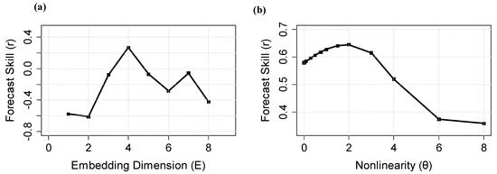
Figure 2.
Results from univariate analysis of hairtail catch by (a) simplex projection and (b) S-map.
For this purpose, the relationships between hairtail catch and six environmental factors are depicted in Figure 3, which clearly shows the absence of linear correlation among these variables. Hence, a nonlinear causality test (convergent cross mapping, CCM) is applied to identify the environmental drivers of hairtail catch. If catch is strongly influenced by environmental factors, it will contain information about past environmental states, thus making it possible to estimate past environmental conditions from the time series of catches. It should be noted that if the environmental factors influence hairtail catch with a time lag, it is necessary to predict an appropriately lagged value of the corresponding environment; thus, reasonable evidence of causal interaction could be obtained by cross mapping from hairtail catch to the environment.
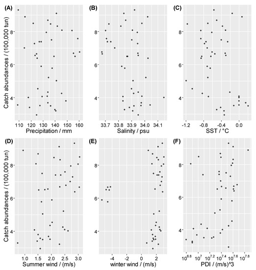
Figure 3.
Relationships (A) between catch abundance and precipitation, (B) between catch abundance and salinity, (C) between catch abundance and SST, (D) between catch abundance and summer wind, (E) between catch abundance and winter wind, (F) between catch abundance and PDI. Here, mm is millimeter; psu is practical salinity units; SST is sea surface temperature; °C is degrees Celsius; m/s is meter per second; PDI is power dissipation index of tropical cyclone.
Table 1 shows the cross-mapping results between catch and the six environmental factors considered in this work, combined with fishing effort. Aside from fishing effort, only two variables show a significant linear correlation with catch abundance, while all six environmental variables show significant nonlinear correlation relationships with catch abundance by cross-map skill. Overall, the effects of the environmental variables on hairtail catch may not be simply one-to-one mapping, and they are much more complex than those captured by CCM analysis or linear correlation function. In order to probe the actual causes influencing catch and elucidate the potential mechanisms of these causative factors, we construct all possible multivariate models by different combinations of all variables demonstrated as significant by CCM.

Table 1.
Results of cross mapping.
4.2. Prediction of Hairtail Abundances: Model Generation and Validation
Although it is usually sufficient to reconstruct a system’s dynamics with a single time series, the system will be incomplete as far as an unclosed system is concerned [13]. In the case of hairtail, fishing effort alone may not skillfully predict future catch abundance because abundance is simultaneously influenced by external environmental factors. Hence, environmental factors act as stochastic external disturbances, which are included in a multivariate reconstruction as coordinates other than catch abundance and fishing effort. It is worth noting that anthropogenic influence on hairtail catch by fishing effort is considered one of the explanatory variables for construction of the EDM models, other than those eliminated in advance by nonlinear regression analysis (e.g., the classical Fox model) [3] because estimation errors of catch abundance would inevitably be introduced into the EDM models by variable-removal operations.
Since the optimal embedding dimension () is set as 4, we limit each multivariate model up to four coordinates to make the system analysis tractable; that is, except for the objective variate (catch abundance) and the anthropogenic factor (fishing effort), there are, at most, two additional environmental variables included in each model, where each environmental coordinate is a 0-, 1-, 2-, 3-, 4-, or 5-year lag of each environmental variable. We set the longest time lags at 5 years, as in reference [2], which is based on the cycle of nutrient circulation among ecosystems. The coordinate of fishing effort is set as a 0-year lag. We use all variables listed in Table 1 (fishing effort and the six other environmental variables) and generate 8474 possible multivariate models (1 one-dimension model, 37 two-dimension models, 666 three-dimension models, and 7770 four-dimension models). In a sense, each model offers a particular perspective on hairtail dynamics based on differing direct or indirect indicators of possible mechanisms. Due to data limitations, we divide the raw data into four parts (1977–1986, 1987–1997, 1998–2007, and 2008–2018) and use the leave-one-out cross-validation method to evaluate model performance. Next, we rank all the models depending on a combination of, which have been shown to perform well in out-of-sample tests [14].
The best three models selected based on the metrics are: A1 [catch(t), fishingeffort(t), salinity(t), summw(t−5)], A2 [catch(t), fishingeffort(t), summw(t), summw(t−5)], and A3 [catch(t), fishingeffort(t), SST(t−3), Preci(t−5)]. As shown in Figure 4, forecast accuracy for these models exceeds 0.93 (= 0.941, 0.938, and 0.937, respectively, at ), and their forecast errors are lower than 0.7 (MAE = 0.661, 0.641, and 0.649, respectively), where fishing effort has been shown to be the common variable, and the variables (salinity(t), summw(t−5), summw(t), sst(t−3), and preci(t−5)) are identified as the most important external environmental factors determining catch abundance. Model A1, <catch(t), fishingeffort(t), salinity(t), summw(t−5)>, shows the best prediction performance in terms of the combination of two metrics from Figure 4.
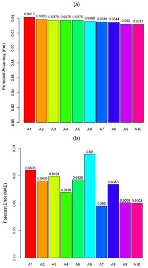
Figure 4.
The selected best ten models: (a) forecast skill (rho) (b) forecast error (MAE).
To validate performance of the selected models, we predict catch abundance during the period from 2008 to 2018 by EDM models constructed with the data during the period from 1977 to 2007. All three models yield statistically significant predictions with p < 0.05. Figure 5 clearly shows the excellent prediction performance of these models, which are closely aligned to the observed trends in catch abundance data. However, there are still some discrepancies between observed and prediction points in each model, such as 2016 by models A2 and A3, 2017 by model A3, and 2018 by model A2. These prediction errors might be explained by an insufficient length of the time series of data used in construction of the EDM models.
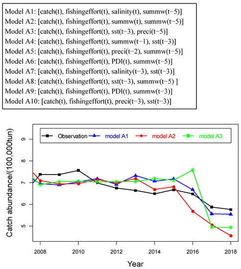
Figure 5.
Out-of-sample prediction of catch abundance by the best three multivariate models.
4.3. Comparison of Catch Forecast Models
In this section, we compare performance of the EDM models with that of traditional parametric models (e.g., linear regression models). To ensure fair comparison of the two methods, we employ the same variables used in EDM models to build the linear regression models. We also use the same evaluation metrics for comparison of the performance of EDM models with that of linear regression models. The results of this comparison are shown in Figure 6. From Figure 6a–c, it can be observed that the best three EDM models have significantly higher prediction accuracy than that of the corresponding linear regression models. Thus, it can be concluded that the nonparametric EDM models, with the flexibility to describe nonlinear dynamic systems, overwhelmingly outperform linear regression models in complex nonlinear systems.
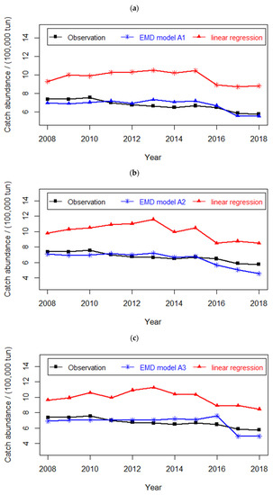
Figure 6.
Comparisons of the prediction: (a) between EDM model A1 and liner regression model (b) between EDM model A2 and liner regression model (c) between EDM model A3 and liner regression model.
5. Discussion
5.1. Environmental Factors
Attempts to reveal the environmental factors affecting hairtail abundance have been made by employing linear regression analysis [11]. However, to the best of our knowledge, these earlier studies did not yield conclusive insights into the nonlinear relationships between hairtail catch abundance and environmental factors, although nonlinear dynamics are ubiquitous in marine ecosystems [35]. Since 1988, use of high-intensity fishing gear has sharply increased, including in hairtail fishing. Fishing effort of hairtail also increased rapidly during this period. Because of these changes in fishing practice, catches of hairtail initially increased from 1988 to 2000 (Figure 1); however, catch abundance of hairtail in the East China Sea has generally declined since 2000, due to years of overfishing.
Aside from the influence of fishing effort on catch, environmental factors are believed to influence hairtail catch. In this work, we demonstrate that EDM models incorporating environmental variables outperform models that consider fishing effort alone. Using multivariate EDM, we conclude that salinity, summer monsoon, SST, precipitation, and PDI of tropical cyclones can be used as variables in the ten best EDM models, as shown in Figure 4.
It is well known that the relationship between environmental factors and fish production is probably linked to ecosystem nutrient cycling. The nutrient supply in primary production is influenced mainly by environmental factors. The saline water flowing from the Kuroshio Current to the ECS shelf is recognized as a rich source of nutrients, including a high concentration of nitrate [39]. It provides abundant organic-matter exporting from the cross-shelf into the deep sea and makes the ECS shelf an area of high production. The summer monsoon season prevails from June to August, coinciding with peak runoff in the Changjiang River [40]. The Changjiang runoff is highly enriched in nitrate and silicate, while the offshore and subsurface water masses are rich in phosphate. In enhancing mixing of these water masses, the summer monsoon supplies abundant nutrients to these waters, thus enhancing primary production. This effect is also reflected in the positive correlation seen between catch and summer monsoon, as shown in Table 1.
Water temperature is one of the vital factors for successful fish reproduction and growth [41]. The increase in water temperature can enhance phytoplankton photosynthesis and increase primary production overall. Finally, it promotes plentiful food availability to support hairtail growth. Terrestrial precipitation is often associated with nutrient richness by inducing river runoff, which generates very high nutrient input to the ECS. Hence, water temperature, combined with terrestrial precipitation, could largely influence the total catch.
Although “tropical cyclones” is not a variable included in the three best EDM models, it does appear as a relevant factor in models A6 and A9, and it could be an important factor in hairtail production in the ECS. Its importance could also be reflected in the positive correlation between catch and the PDI of tropical cyclones shown in Table 1. Tropical cyclones can bring strong winds and heavy rainfall, which result in large increases in nutrients and phytoplankton reproduction in coastal waters after these storms [42]. Fish production thus also increases accordingly [2].
Figure 4 also demonstrates that the ten different EDM models show similar levels of performance. This similarity reflects a fundamental property of the EDM method: the prediction performance of different models depends only on the information of data [13]. From the above analysis, it is clear that the identified environmental factors have a common effect: an impact on nutrient supply, which is the potential mechanism influencing hairtail catch. The environmental factors discussed above are solely extrinsic indicators of this underlying mechanism.
5.2. EDM for Nonlinear Analysis
Marine ecosystems are complex nonlinear systems framed by the intersection of a diverse set of physical, chemical, and biological components [32,43]. Our analysis of the dataset by EDM suggests the nonlinear nature of the marine system. To date, efforts investigating the effects on hairtail abundance of fishing effort and environmental variability have mostly focused on machine-learning regression techniques [1,8]. Those models investigate the relationship based on an assumption of linear correlation. In nonlinear systems, the correlation among the given variables is nonlinear, and “mirage correlations” frequently occur, making traditional regression techniques ill-suited to describing physical behaviors of these systems. In our work, the correlation among these variables is nonlinear (Figure 3), and therefore, nonlinear tools are necessary and suitable to reveal the relationship between variables.
As demonstrated in this work, EDM has the advantages in identifying complex causes and predicting catch abundance in marine systems. The good performance of EDM achieved offers an alternative for researchers to reveal the relationship between fluctuations in fish catch and variability in both fishing effort and marine environmental conditions. For fishery managers, skillful nonlinear tools, e.g., the EDM approach, also enable them to obtain accurate prediction of fish catch, thus assisting them in instituting reasonable fishery policies [44].
EDM is fundamentally a data-driven approach. It uses time-series data to reconstruct an attractor and then identify the environmental variables based on the attractor. Thus, sufficient length of data is a critical issue to the recovery of dynamics. As suggested by Sugihara et al., more than 35–40 points might be a necessary requirement [35]. In our work, we used yearly time series data with 42 observations for each variable, which satisfies the minimum data requirement of EDM. Thus, in view of insufficient available data, it is almost impossible for us to conduct careful investigations on whether the performance of EDM can be enhanced by lengthening time-series data. Hence, such investigations will be considered in future work. Moreover, if high-resolution data (e.g., sampled monthly) can be provided, much more information may be extracted by constructing much more compact models.
6. Conclusions
In this paper, an equation-free method (EDM) has been introduced to explore the key factors influencing catch abundance of hairtail in the ECS and to elucidate the potential mechanisms underlying these effects. First, we applied the simplex method to select the optimal embedding dimension. Then, we applied a convergent cross-mapping method to carry out a causality analysis of hairtail catch abundances. We then constructed multivariate EDM models and applied a combination of metrics to evaluate the performance of these models. Finally, we compared the predictive performance of EDM models and parametric models using historical data; EDM models overwhelmingly outperformed the parametric models.
We find that there would more than one EDM model for a given set of data, which show similar excellent predictive performance. Our model analysis suggests the potential mechanisms explaining the relationships between environmental factors and catch abundance. Impact on nutrient supply is a potential mechanism influencing hairtail catch.
Author Contributions
Conceptualization, J.H. methodology, J.H.; software, J.H.; validation, J.H.; resources, P.W.; data curation, P.W.; writing—original draft preparation, J.H.; writing—review and editing, H.Z.; project administration, J.H.; funding acquisition, J.H., P.W. and H.Z. All authors have read and agreed to the published version of the manuscript.
Funding
This research was supported in part by the Fundamental Research Funds for Zhejiang Provincial Universities and Research Institutes (No. 2019J00046). And this research was also supported by the Bureau of Science and Technology of Zhoushan (No: 2016C41014, No: 2018C21020) and by the National Key Research and Development Projects of China (No. 2019YFD0900901).
Acknowledgments
This research was supported in part by the Fundamental Research Funds for Zhejiang Provincial Universities and Research Institutes (No. 2019J00046). This research was also supported by the Bureau of Science and Technology of Zhoushan (No: 2016C41014, No: 2018C21020) and by the National Key Research and Development Projects of China (No. 2019YFD0900901).
Conflicts of Interest
The authors declare that they have no known competing financial interests or personal relationships that could have appeared to influence the work reported in this paper.
References
- Sun, P.; Chen, Q.; Fu, C.; Zhu, W.; Li, J.; Zhang, C.; Yu, H.; Sun, R.; Tian, Y. Daily growth of young-of-the-year largehead hairtail (Trichiurus japonicas) in relation to environmental variable in the East China Sea. J. Mar. Syst. 2020, 201, 103243. [Google Scholar] [CrossRef]
- Qiu, Y.; Lin, Z.; Wang, Y. Responses of fish production to fishing and climate variability in the northern South China Sea. Prog. Oceanogr. 2010, 85, 197–212. [Google Scholar] [CrossRef]
- Wang, Y.; Jia, X.; Lin, Z.; Sun, D. Responses of Trichiurus japonicas catches to fishing and climate variability in the East China Sea. J. Fish. China 2011, 35, 1881–1889. (In Chinese) [Google Scholar]
- Jahncke, J.; Saenz, B.L.; Abraham, C.L.; Rintoul, C.; Bradley, R.W.; Sydeman, W.J. Ecosystem responses to short-term climate variability in the Gulf of the Farallones, California. Prog. Oceanogr. 2008, 77, 182–193. [Google Scholar] [CrossRef]
- Zainuddin, M.; Kiyofuji, H.; Saitoh, K.; Saitoh, S.I. Using multi-sensor satellite remote sensing and catch data to detect ocean hot spots for albacore (Thunnus alalunga) in the northwestern North Pacific. Deep Sea Res. II 2006, 53, 419–431. [Google Scholar] [CrossRef]
- Dutta, S.; Chanda, A.; Akhand1, A.; Hazra1, S. Correlation of Phytoplankton Biomass (Chlorophyll-a) and Nutrients with the Catch Per Unit Effort in the PFZ Forecast Areas of Northern Bay of Bengal during Simultaneous Validation of Winter Fishing Season. Turk. J. Fish. Aquat. Sc. 2006, 16, 767–777. [Google Scholar]
- Tian, Y.; Kidokoro, H.; Watanabe, T.; Iguchi, N. The late 1980s regime shift in the ecosystem of Tsushima warm current in the Japan/East Sea: Evidence from historical data and possible mechanisms. Prog. Oceanogr. 2008, 7, 127–1445. [Google Scholar] [CrossRef]
- Yu, H.; Yu, H.; Ito, S.-I.; Tian, Y.; Wang, H.; Liu, Y.; Xing, Q.; Bakun, A.; Kelly, R. Potential environmental drivers of Japanese anchovy (Engraulis japonicus) recruitment in the Yellow Sea. J. Mar. Syst. 2020, 212, 103431. [Google Scholar] [CrossRef]
- Chifamba, P.C. The relationship of temperature and hydrological factors to catch per unit effort, condition and size of the freshwater sardine, Limnothrissa miodon (Boulenger), in Lake Kariba. Fish. Res. 2000, 45, 271–281. [Google Scholar] [CrossRef]
- Ling, J.; Yan, L.; Lin, L.; Li, J.; Cheng, J. Reasonable utilization of hairtail Trichiurus japonicas resource in the East China Sea based on its fecundity. J. Fish. China 2005, 12, 726–730. (In Chinese) [Google Scholar]
- Xu, Z.; Chen, J. Migratory routes of Trichiurus lepturus in the East China Sea, Yellow Sea and Bohai Sea. J. Fish. China 2015, 39, 824–835. (In Chinese) [Google Scholar]
- Liu, Z.-F.; Xu, H.-X.; Zhou, Y.-D. An ameliorative study on the forecast of recruitment stock and catch in winter seasons of hairtail, Trichiurus haumela in the East China Sea. J. Zhejiang Ocean Univ. (In Chinese). 2004, 23, 14–18. [Google Scholar]
- Ye, H.; Beamish, R.J.; Glaser, S.M.; Grant, S.C.H.; Hsieh, C.-H.; Richards, L.J.; Schnute, J.T.; Sugihara, G. Equation-free mechanistic ecosystem forecasting using empirical dynamic modeling. Proc. Natl. Acad. Sci. USA 2015, 112, E1569–E1576. [Google Scholar] [CrossRef] [PubMed] [Green Version]
- Mcgowan, J.; Deyle, E.; Ye, H.; Carter, M.; Peretti, C. Predicting coastal algal blooms in southern California. Ecology 2018, 98, 1419–1433. [Google Scholar] [CrossRef] [PubMed] [Green Version]
- Wang, M.; Yoshimura, C.; Allam, A.; Kimura, F.; Honma, T. Causality analysis and prediction of 2-methylisoborneol production in a reservoir using empirical dynamic modeling. Water Res. 2019, 163, 114864. [Google Scholar] [CrossRef]
- Sarah, G.M.; Hao, Y.; George, S. A nonlinear, low data requirement model for producing spatially explicit fishery forecasts. Fish Oceanogr. 2014, 23, 45–53. [Google Scholar]
- Bureau of Fisheries of the Ministry of Agriculture. China Fishery Statistical Yearbook 1978–2019; China Agricultural Press: Beijing, China, 2019. [Google Scholar]
- Maunder, M.N.; Sibert, J.R.; Fonteneau, A.; Hampton, J.; Kleiber, P.; Harley, S.J. Interpreting catch per unit effort data to assess the status of individual stocks and communities. ICES J. Mar. Sci. 2006, 63, 1373–1385. [Google Scholar] [CrossRef]
- Poulsen, R.T.; Holm, P. What Can Fisheries Historians Learn from Marine Science? The Concept of Catch per Unit Effort (CPUE). Int. J. Marit. Hist. 2007, 19, 89–112. [Google Scholar] [CrossRef]
- Maunder, M.N.; Punt, A.E. Standardizing catch and effort data: A review of recent approaches. Fish. Res. 2004, 70, 141–159. [Google Scholar] [CrossRef]
- Maunder, M.N.; Thorson, J.T.; Xu, H.; Oliveros-Ramos, R.; Hoyle, S.D.; Tremblay-Boyer, L.; Lee, H.H.; Kai, M.; Chang, S.K.; Kitakado, T.; et al. The need for spatio-temporal modeling to determine catch-per-unit effort based indices of abundance and associated composition data for inclusion in stock assessment models. Fish. Res. 2020, 229, 105594. [Google Scholar] [CrossRef]
- Harley, S.J.; Myers, R.A.; Dunn, A. A meta-analysis of the relationship between catch-per-unit-effort and abundance. Can. J. Fish. Aquat. Sci. 2001, 58, 1705–1772. [Google Scholar] [CrossRef]
- Thorson, J.T.; Fonner, R.; Haltuch, M.A.; Ono, K.; Winker, H. Accounting for spatiotemporal variation and fisher targeting when estimating abundance from multispecies fishery data. Can. J. Fish. Aquat. Sci. 2017, 74, 1794–1807. [Google Scholar] [CrossRef] [Green Version]
- Korman, J.; Yard, M.D. Effects of environmental covariates and density on the catchability of fish populations and interpretation of catch per unit effort trends. Fish. Res. 2017, 189, 18–34. [Google Scholar] [CrossRef] [Green Version]
- Kai, M.; Thorson, J.T.; Piner, K.R.; Maunder, M.N. Spatio-temporal variation in size-structured populations using fishery data: An application to shortfin mako (Isurus oxyrinchus) in the Pacific Ocean. Can. J. Fish. Aquat. Sci. 2017, 74, 1765–1780. [Google Scholar] [CrossRef] [Green Version]
- Kai, M. Spatio-temporal changes in catch rates of pelagic sharks caught by Japanese research and training vessels in the western and central North Pacific. Fish. Res. 2019, 216, 177–195. [Google Scholar] [CrossRef]
- Nielsen, J.R.; Kristensen, K.; Lewy, P.; Bastardie, F. A statistical model for estimation of fish density including correlation in size, space, time and between species from research survey data. PLoS ONE 2014, 9, e99151. [Google Scholar]
- Punt, A.E.; Walker, T.I.; Taylor, B.L.; Pribac, F. Standardization of catch and effort data in a spatially-structured shark fishery. Fish. Res. 2000, 45, 129–145. [Google Scholar] [CrossRef]
- Emanuel, K. Increasing destructiveness of tropical cyclones over the past 30 years. Nature 2005, 436, 686–688. [Google Scholar] [CrossRef]
- Liu, H.; Fogarty, M.J.; Glaser, S.M.; Altman, I.; Hsieh, C.-H.; Kaufman, L.; Rosenberg, A.A.; Sugihara, G. Nonlinear dynamic features and co-predictability of the Georges Bank fish community. Mar. Ecol. Prog. Ser. 2012, 464, 195–207. [Google Scholar] [CrossRef] [Green Version]
- Hsieh, C.H.; Glaser, S.M.; Lucas, A.J.; Sugihara, G. Distinguishing random environmental fluctuations from ecological catastrophes for the North Pacific Ocean. Nature 2005, 435, 336–340. [Google Scholar] [CrossRef]
- Glaser, S.M.; Fogarty, M.J.; Liu, H.; Altman, I.; Hsieh, C.-H.; Kaufman, L.; MacCall, A.D.; Rosenberg, A.A.; Ye, H.; Sugihara, G. Complex dynamics may limit prediction in marine fisheries. Fish Fish. 2014, 15, 616–633. [Google Scholar] [CrossRef]
- Horan, R.D.; Fenichel, E.P.; Drury, K.L.S.; Lodge, D. Managing ecological thresholds incoupled environmental-human systems. Proc. Natl. Acad. Sci. USA 2011, 108, 7333–7338. [Google Scholar] [CrossRef] [Green Version]
- Deyle, E.R.; Sugihara, G. Generalized theorems for nonlinear state space reconstruction. PLoS ONE 2011, 6, e18295. [Google Scholar] [CrossRef] [PubMed]
- Sugihara, G.; May, R.; Ye, H.; Hsieh, C.-H.; Deyle, E.; Fogarty, M.; Much, S. Detecting causality in complex ecosystems. Science 2012, 338, 496–500. [Google Scholar] [CrossRef] [PubMed]
- Takens, F. Detecting strange attractors in turbulence. In Symposium on Dynamical Systems and Turbulence; Lecture Notes in Mathematics; Rand, D.A., Young, L.S., Eds.; Springer: Berlin/Heidelberg, Germany, 1981; Volume 898, pp. 366–381. [Google Scholar]
- Sugihara, G.; May, R.M. Nonlinear forecasting as a way of distinguishing chaos from measurement error in time series. Nature 1990, 344, 734–741. [Google Scholar] [CrossRef] [PubMed]
- Van Nes, E.H.; Scheffer, M.; Brovkin, V.; Lenton, T.M.; Ye, H.; Deyle, E.; Sugihara, G. Causal feedbacks in climate change. Nat. Clim. Chang. 2015, 5, 445–448. [Google Scholar] [CrossRef]
- Li, Y.H. Material exchange between the East China Sea and the Kuroshio Current. Terr. Atmos. Ocean. Sci. 1994, 5, 625–631. [Google Scholar] [CrossRef]
- Shi, Y.-L.; Yang, W.; Ren, M.-E. Hydrological characteristics of the Changjiang and its relation to sediment transport to the sea. Cont. Shelf Res. 1985, 4, 5–15. [Google Scholar]
- Morgan, M.J.; ORiordan, R.M.; Culloty, S.C. Climate change impacts on potential recruitment in an ecosystem engineer. Ecol. Evol. 2013, 3, 581–594. [Google Scholar] [CrossRef]
- Zheng, G.M.; Tang, D.L. Offshore and nearshore chlorophyll increases induced by typhoon winds and subsequent terrestrial rainwater runoff. Mar. Ecol. Prog. Ser. 2007, 333, 61–74. [Google Scholar] [CrossRef] [Green Version]
- Glaser, S.M.; Ye, H.; Maunder, M.; MacCall, A.; Fogarty, M.J.; Sugihara, G. Detecting and forecasting complex nonlinear dynamics in spatially-structured catch-per-unit effort time series for North Pacific albacore (Thunnus alalunga). Can. J. Fish. Aquat. Sci. 2011, 68, 400–412. [Google Scholar] [CrossRef]
- Munch, S.B.; Giron-Nava, A.; Sugihara, G. Nonlinear dynamics and noise in fisheries recruitment: A global meta-analysis. Fish Fish. 2018, 19, 964–973. [Google Scholar] [CrossRef]
Publisher’s Note: MDPI stays neutral with regard to jurisdictional claims in published maps and institutional affiliations. |
© 2021 by the authors. Licensee MDPI, Basel, Switzerland. This article is an open access article distributed under the terms and conditions of the Creative Commons Attribution (CC BY) license (https://creativecommons.org/licenses/by/4.0/).