Spatial Modeling of Potential Lobster Harvest Grounds in Palabuhanratu Bay, West Java, Indonesia

Abstract

Palabuhanratu Bay is a location in the southern part of Java Island with a high lobster population. Based on field observation, the lobster population in Palabuhanratu Bay is dominated by Panulirus homarus (green sand lobster), Panulirus versicolor (bamboo lobster), Panulirus penicillatus (black lobster), and Panulirus ornatus (pearl lobster). This study aimed to develop a spatial model using satellite-derived data to predict potential lobster harvest grounds in Palabuhanratu Bay. The Earth observational satellite data used were multispectral Landsat 8-SR imagery, and information about chlorophyll-a, salinity, total suspended solids (TSSs), sea surface temperature (SST), and distance from the coastline was extracted. Multiple linear regression was applied to build the prediction model, which was validated using 10-fold cross-validation. The result of the lobster harvest prediction model agreed with the root-mean-square error (RMSE) and adjusted R² values of 0.326 and 0.708, respectively. The distribution of lobsters was strong at the following preferred ranges: chlorophyll-a: 1.1–1.7 mg/m³; salinity: 20.2–23.7 ppt; TSS: 40–56.4 mg/L; SST: 29.5–29.9 °C; and distance from the coastline: 500–4700 m. In this study, the habitats of four species of lobsters and their relationships with satellite-derived parameters were evaluated.

1. Introduction

Sukabumi Regency is a potential lobster-producing area in Indonesia, specifically in the Palabuhanratu Bay area of West Java Island (Figure 1). The waters of Palabuhanratu are characteristic of coral waters, the main habitat of lobsters [1]. Lobsters are a potential fishery commodity and are important for export because of their economic value [2]. According to the Director General of Indonesian Fishery Product Processing and Marketing, in 2014, 69.4% of Indonesia’s lobsters were exported to China and 22.6% were exported to Taiwan. These exports collectively weighed 3427 tonnes and were worth US$ 42.8 million [3]. The majority of lobsters caught in Palabuhanratu Bay are Panulirus homarus (green sand lobster), Panulirus versicolor (bamboo lobster), Panulirus penicillatus (black lobster), and Panulirus ornatus (pearl lobster). [4]. Lobsters have been caught at several locations around the Palabuhanratu Bay area, including the waters of Cisolok, Karang Hawu, Karang De’et, Cimandiri, Sanggra Wayang, Jampang, and Karang Hantu. In addition to being potential lobster harvest grounds, Palabuhanratu Bay also has the potential for lobster cultivation. Palabuhanratu Bay is located in West Java Province, Indonesia, between the coordinates 06°57′ S, 106°22′ E and 07°07′ S, 106°33′ E. Palabuhanratu Bay is bordered by the Cisolok, Cikakak, Palabuhanratu, and Simpenan districts (Figure 1), and it is the largest bay along the southern coast of Java Island [5].

Oceanographic conditions, such as the physical and chemical aspects of seawater, determine the productivity of the waters [6]. Lobster habitats are dependent on chemical aspects of the coastal environment and are spatially distributed along the coastline. The biology of lobsters is influenced by oceanographic conditions, including chlorophyll-a [7,8], TSSs (total suspended solids) [9,10], temperature [11,12,13], substrate [14,15], salinity [16], and other environmental variables [17,18]. It is time-consuming and expensive to conduct observations of oceanographic conditions using conventional methods over a wide area; therefore, remote sensing on a large scale is more cost-effective than field surveys for the periodic collection of large-scale habitat data [19]. Remote sensing and geographic information systems can be applied to extract coastal and marine parameters related to the characteristics of lobster habitats by identifying useful types of data, approaches, and algorithms as quick solutions for water quality assessments.

Remote sensing data on multispectral images, such as those collected by Landsat 8 satellite imaging, are useful for marine monitoring because the spatial resolution of Landsat 8 is 30 m [20], which is regarded as medium resolution and can be applied to a wide area of coverage. The availability of consistent data every 16 days [20] gives Landsat 8 the ability to support research that requires a series of observations. Landsat 8 also possesses various bands as tools to implement marine monitoring algorithms, such as the red, green, blue, and near infra-red bands [20], which can detect chlorophyll-a, salinity, and total suspended solids (TSSs). Landsat 8 also possesses the thermal infrared sensor band [20], which can detect sea surface temperature (SST) values. Landsat-8-derived oceanographic information has been widely used to model the potential occurrence of marine resources such as shrimp, tuna, and other pelagic species. Among the advantages of satellite-derived oceanographic information are free access and timeseries availability, which make this type of information suitable for monitoring and operational purposes.

Lobsters are among the marine resources with high potential for commercialization. Operational monitoring of their abundance is one of the ways to sustain their populations. Research on spatial modeling of lobsters has mostly been carried out on lobster habitats and distributions. The identification of lobsters’ preferred habitats [21] can be linked to the density, abundance, and biomass of each habitat type to allow the prediction of the spatial distribution of lobsters in a particular area [22]. The distribution of lobsters can be used to determine the relationship between the population and marine conservation areas that can support lobsters [23]. In Indonesia, the lobster studies that have been conducted have been limited to biodiversity studies [24,25], spatial bio-economic models [26,27], social ecology aspects [28], population density [29], and habitat suitability [16]. The research on lobsters in Indonesia has not yet focused on the spatial prediction of potential lobster harvest areas. This paper takes a new look at the prediction of potential lobster harvest grounds using a spatial linear regression model based on a recorded capture dataset, as well as satellite-derived data.

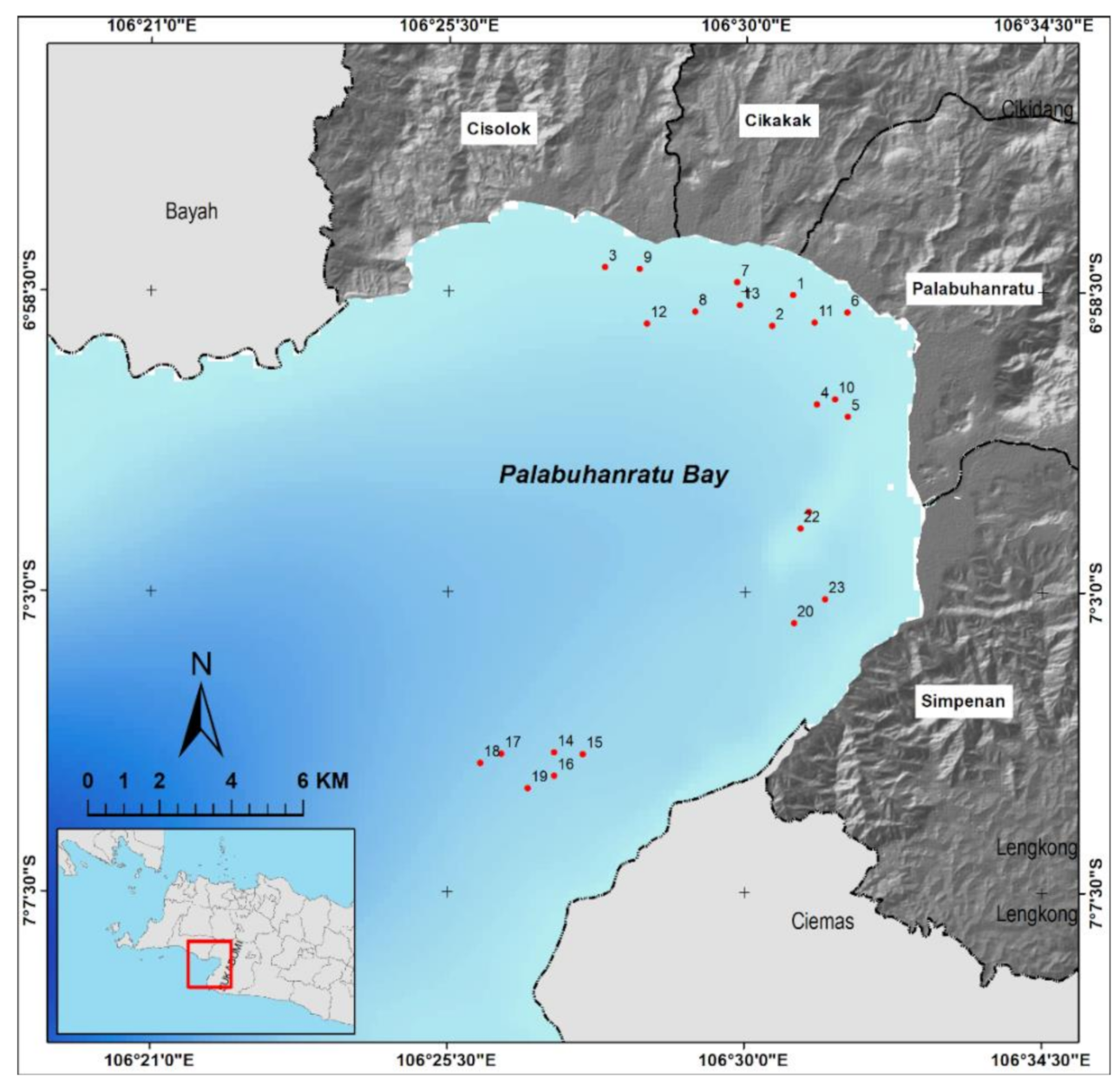
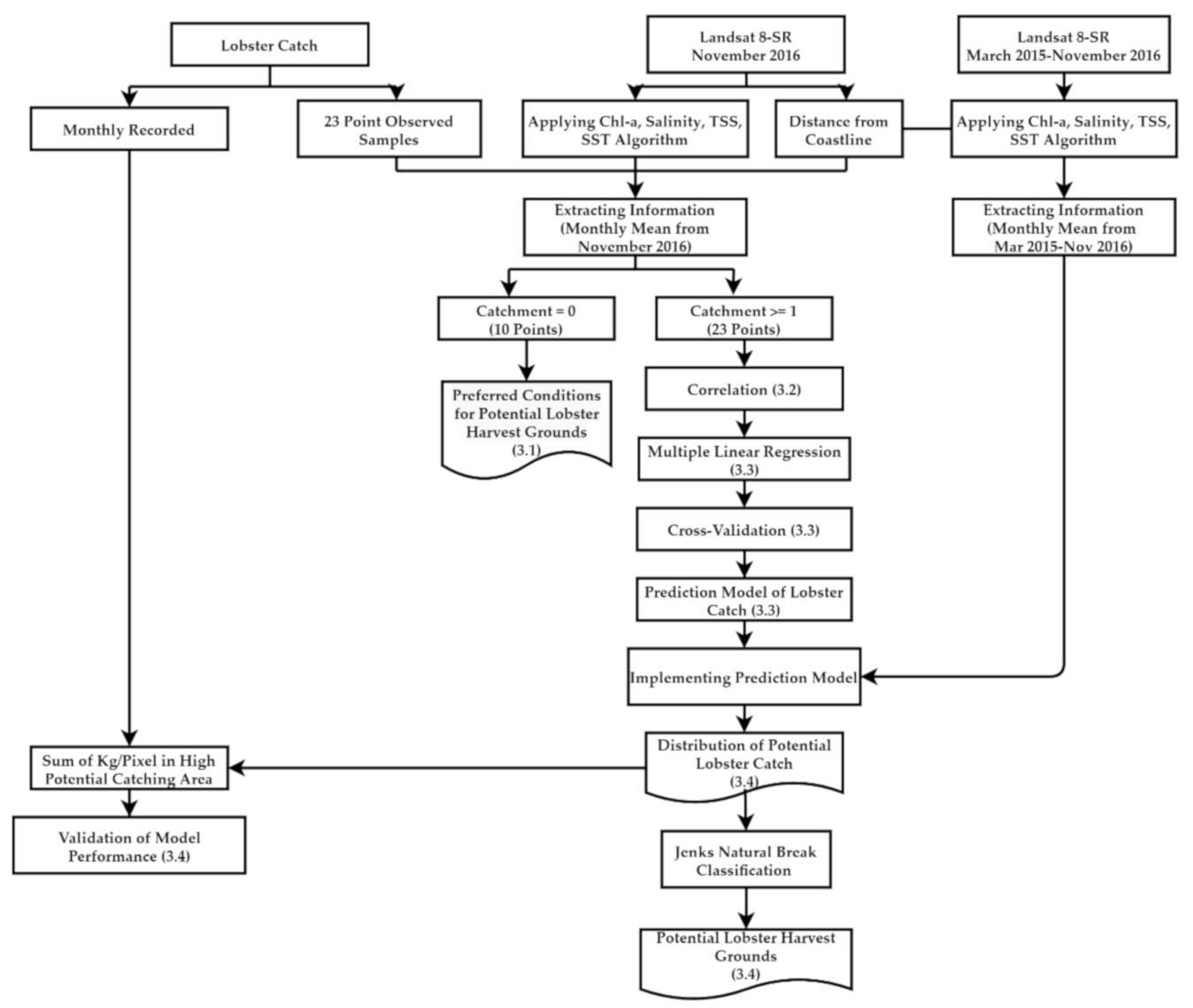
2. Materials and Methods

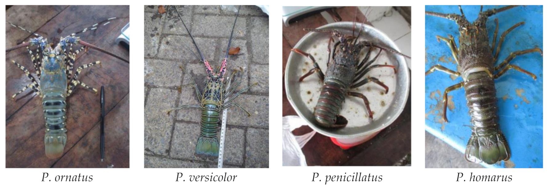
2.1. Lobster Catches

This study used data from lobster catches at 23 sample points taken during November 2016 [30] and monthly lobster harvest data taken from March 2015 to November 2016. The retrieval of data on the numbers, weight, and species of lobsters harvested in Palabuhanratu Bay was carried out from March 2015 to November 2016. The 23 observation points were collected to determine the number, type, sex, carapace length, weight, and exact location of lobsters by following the route of a lobster catching trip conducted by fishermen. The lobsters were collected using a single-layer net consisting of polyamide with a mesh size of 5 inches (12.7 cm) [30], equipped with buoys, weights, and ropes to form a basic gill net [30]. The monthly data on lobster catches was obtained in the form of lobster number data, which we converted into kilograms by multiplying the number of lobsters by the average weight of each type of lobster caught. These data originated from the purchase of lobsters from fishermen by the data collectors [30].

The types of lobsters caught in Palabuhanratu Bay are the green sand lobster (Panulirus homarus), bamboo lobster (Panulirus versicolor), black lobster (Panulirus penicillatus), and pearl lobster (Panulirus ornatus), as shown in Figure 2. The sand lobster has a maximum body length of 31 cm with an average body length of 20–25 cm and a carapace length of approximately 12 cm [31]. This species has a greenish or brownish base color with bright spots scattered over the surface of the abdominal segment and white spots on the legs [31]. The bamboo lobster has an average body length of no more than 30 cm with a maximum body length of 40 cm [31]. This species is characterized by a green head and abdomen with a black carapace [31]. The black lobster has a body length of 20–30 cm with a maximum size of 40 cm [32]. This species has a dark blue and black body, irregular spots on the abdomen, and a white stripe on the legs [32]. Pearl lobsters can reach a body length of 60 cm with an average of 20–35 cm [32]. This species has a greenish and slightly bluish body in the carapace, and each segment of the abdomen is covered with a thick dark line located in the middle, with medium-sized yellowish patches [32].

2.2. Satellite-Derived Parameters

Data on chlorophyll-a, salinity, TSSs, SST, and distance from the coastline were obtained from Landsat 8 Surface Reflectance (Landsat 8-SR) imagery. Landsat 8-SR is generated from a special software called Landsat 8 Surface Reflectance Code (LaSRC). LaSRC generates the top of atmosphere (TOA) reflectance and the TOA brightness temperature (BT) using calibration parameters from the metadata [33]. Landsat 8-SR has a spatial resolution of 30 m per pixel [33], which became the spatial resolution basis for developing the spatial model. The Landsat 8-SR time series images were accessed using the Google Earth Engine app [34]. The chemical conditions of the seawater were extracted with various algorithms implemented using the Landsat 8-SR satellite imagery. The value of chlorophyll-a was estimated using the Wibowo (1994) algorithm following Firdaus (2017) [35]; the salinity was estimated using the Cilamaya (2019) algorithm [36]; the TSSs were estimated using the algorithm of Budhiman et al. (2004) [37]; and the SST was estimated using the algorithm of Syariz et al. (2015) with band 11 [38]. These algorithms (

Table 1. Selected algorithms for predicting lobster catches.

Algorithms
$\mathrm{Chl}-\mathrm{a}\left(\mathrm{mg}/{\mathrm{m}}^3\right)=0.2818\times {\left(\frac{\mathrm{Red}+\mathrm{NIR}}{\mathrm{Green}}\right)}^{3.497}$	(1)
$\mathrm{Salinity}\left(\mathrm{ppt}\right)=139.556970+(86.21318\times \mathrm{Ln}(\mathrm{Blue}\left)\right)-(24.62518\times$Ln (Red))	(2)
$\mathrm{TSS}\left(\mathrm{mg}/\mathrm{L}\right)=7.9038\times \exp \left(23.942\times \mathrm{Red}\right)$	(3)
$\mathrm{SST}(℃)=-0.0197\mathrm{BT}{11}^2+0.2881\mathrm{BT}11+29.004$	(4)

) have been validated previously and are in good agreement with the field measurement dataset [39].

Furthermore, from the satellite images, the 23 observed sample values and the 23 extraction values for chlorophyll-a, salinity, TSSs, SST, and distance from the coastline were tested using multiple linear regression to produce a predictive model for lobster harvests (Figure 3). The extraction values from Landsat 8-SR were calculated by the mean of monthly imagery for November 2016 because the observation time did not coincide with the date the satellite image was taken. The prediction model was validated using the cross-validation (CV) method. If the resulting model showed good results, this meant that the prediction model could be implemented in other satellite images, which would produce a lobster catch distribution prediction. The distribution of these predictions was then classified into three classes with the Jenks Natural Break Classification method [40], which produced a predicted area for potential lobster catches. The kilograms per pixel were summed in a high-potential harvest area to validate model performance with monthly recorded data. To determine preferred conditions for the potential lobster harvest grounds, we used only 10 samples of lobsters that could be found and that represented the preferred water quality conditions for lobsters (Figure 3).

2.3. Multiple Linear Regression

Multiple linear regression analysis fits a linear relationship between two or more independent variables (X₁, X₂, …, X_n) and a dependent variable (Y). This analysis is used to determine the direction of the positive or negative relationship between the independent variables and the dependent variable, and to predict the value of the independent variables if the value of the dependent variable increases or decreases. Simple or multiple linear regression models can be obtained by estimating the parameters with certain methods. The maximum likelihood estimation method and the ordinary least squares method can be used to estimate the parameters of a simple linear regression model or a multiple linear regression model. [41]. The general form of the multiple linear regression model is as follows [41]:

Y = a + b₁X₁+ b₂X₂ +…..+ b_nX_n.

(5)

where Y is the number of lobsters caught, a is offset, X is oceanographic derived information, i.e., chlorophyll-a, salinity, TSSs, SST, depth, and distance from the coastline, and b_n is a coefficient determined by linear regression analysis using a set of lobster catch data with the oceanographic derived information.

The prediction model generated from the regression must be validated with 10-fold CV, which is one of the recommended CV methods for choosing the best model because it tends to provide less biased estimates of accuracy compared to other types of CVs [42]. By default, 10-fold CV uses 75% of the data for training and 25% of the data for testing. Moreover, this study tested several options of data training and testing separation. This model performs training and data testing 10 times and generates predictive errors from each model installation, which is then averaged to determine the predictive statistics for the model. The results can be seen in the values of the root-mean-square error (RMSE) and the coefficient of determination (R²) in the following equation [43,44]:

$$\mathrm{RMSE}={\left(\frac{\sum (y_i-\widehat{y_i)}}{n}\right)}^{1/2},$$

(6)

where y is the observed value, ŷ is the predicted value, i is the sequence of data in the database, and n is the total amount of data.

$${\mathrm{R}}^2={\left(\frac{n\left(\sum xy\right)-\left(\sum x\right)\left(\sum y\right)}{\sqrt{[n\left(\sum x_2\right)-{(\sum x)}^2[n\left(\sum y_2\right)-\left(\sum y{)}^2\right]}}\right)}^2,$$

(7)

where y is the dependent variable, x is the independent variable, and n is the total amount of data.

The estimation algorithms were then implemented using the Landsat 8-SR satellite imagery from November 2016, which produced the data on the distribution of chlorophyll-a, salinity, TSSs, and SST. We then extracted the values of the distribution of chlorophyll-a, salinity, TSSs, SST, depth, and distance from the coastline based on the sample points of the lobster catch data. All extraction values and lobster catch data were used for multiple linear regression tests to produce a predictive spatial model of lobster harvest potential. The multiple linear regression was implemented with the spatial dataset of oceanographic derived parameters to create the spatial distribution of potential lobster harvest areas. Then, cross-validation was carried out on the model to evaluate its performance. The prediction model and the estimation algorithms were then implemented using the Landsat 8-SR satellite imagery from March 2015 to November 2016 to determine the distribution of lobster harvest potential. All of these processes were run in the Google Earth Engine [34] for image preprocessing, extracting the oceanographic derived information. For the correlation analysis, multiple linear regression, and accuracy assessment, this used “stats” [45], “raster” [46], and “gdal” [47] packages for R calculations. The distribution of potential catches can be analyzed by classifying areas as low, medium, or high potential, so we grouped them into three classes with the Jenks Natural Break Classification. The Jenks Natural Break Classification determines the best value for arranging data into different classes by minimizing the average deviation of each class from the class mean while maximizing the deviation of each class from the mean of the other groups [40].

3. Results

3.1. Preferred Conditions for Potential Lobster Harvest Grounds

Lobsters were found under specific environmental conditions (10 observation points with lobsters caught = 0) and, under some conditions, lobsters were not found (13 points with lobsters caught ≥1). Figure 4 shows that the distribution of lobsters was strongly associated with the following ranges of environmental parameters: chlorophyll-a: 1.1–1.7 mg/m³; salinity: 20.2–23.7 ppt; TSSs: 40–56.4 mg/L; SST: 29.5–29.9 °C; and distance from the coastline: 500–4700 m. In the highest lobster harvest areas, the salinity and TSS also had the highest ranges of values.

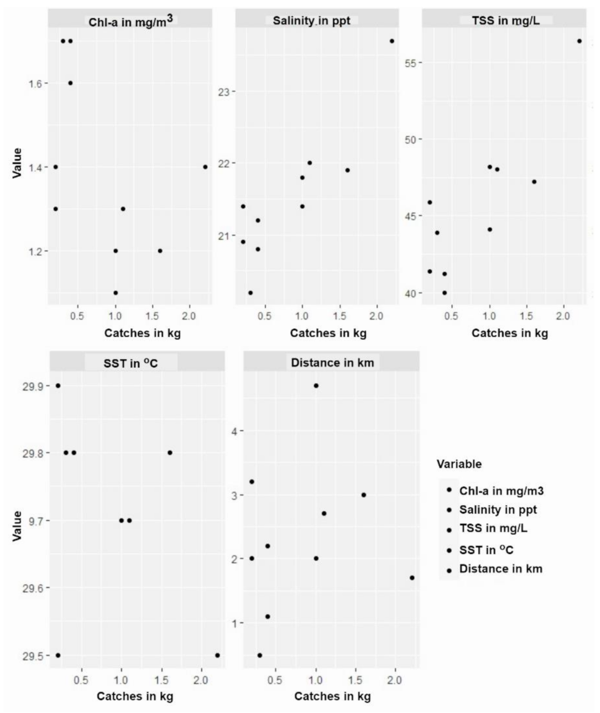
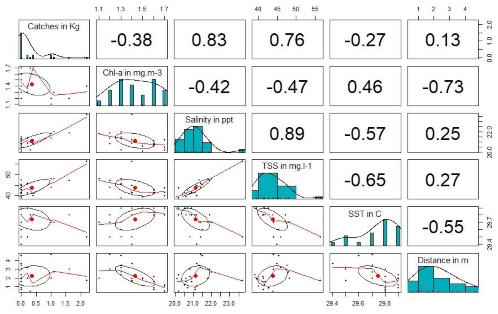
3.2. Correlation between Potential Lobster Harvest Grounds and Environmental Factors

There were very strong relationships between lobster catches and the salinity and TSS variables (Figure 5). This is because the level of salinity can affect the metabolic response of lobsters, which, in turn, affects their distribution, movement, and migration patterns [18]. The level of TSSs can affect the abundance of phytoplankton and water turbidity levels [31], and lobster habitats are located in turbid waters [1]. In addition, there were adequate relationships between lobster catches and two other variables, SST and chlorophyll-a, while there was a weak relationship between lobster catches and distance from the coastline. The number of lobsters caught at 23 sample points was used as the dependent variable when building a predictive model for lobster harvest potential in this study.

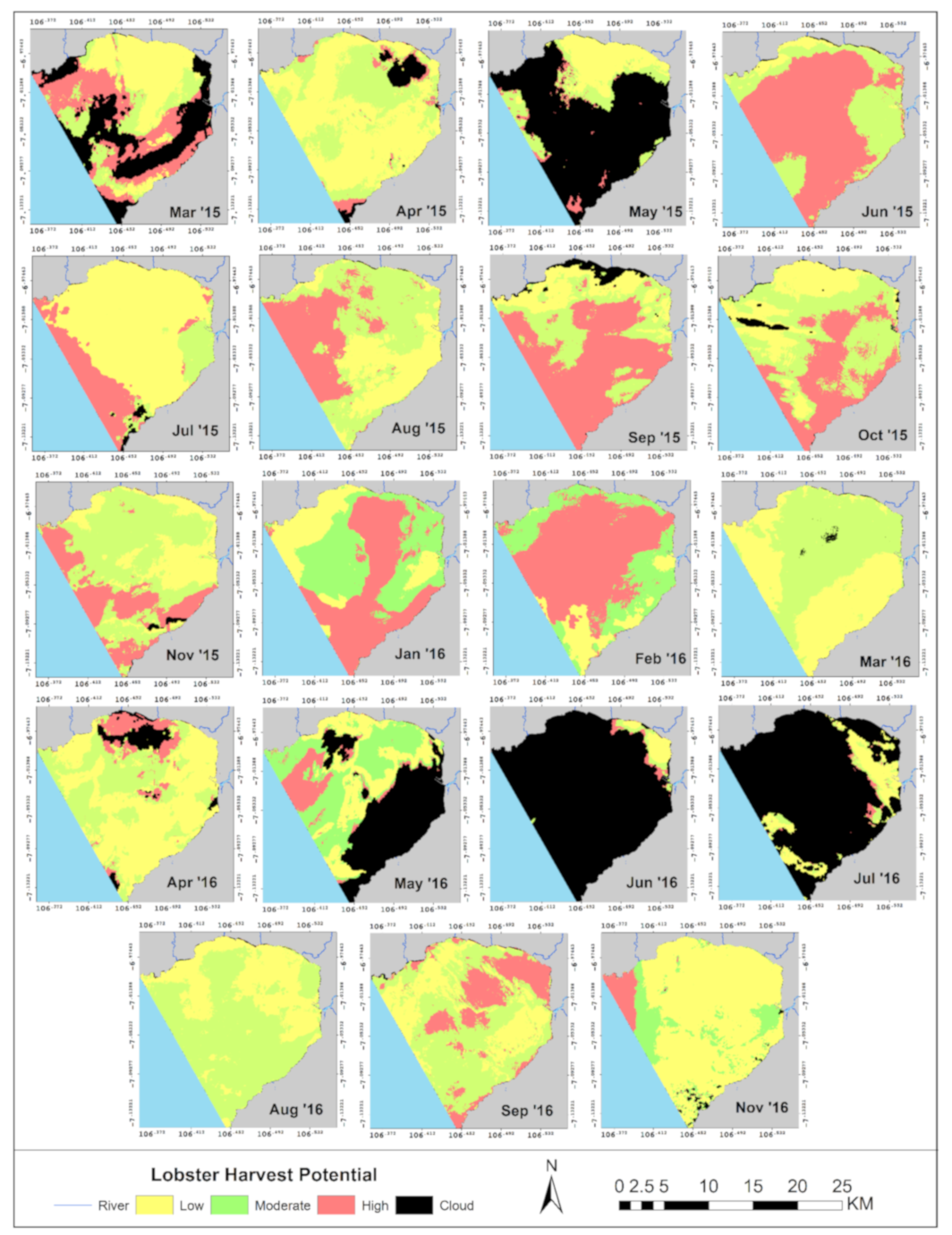
3.3. Spatial Prediction of Potential Lobster Harvest Grounds

The model was calculated using 23 points of lobster catch data: the average values of chlorophyll-a, salinity, TSSs, and SST in November 2016, derived from Landsat 8-SR satellite imagery using estimator algorithms; and distance-from-coastline data. The combination of chlorophyll-a, salinity, TSSs, SST, and distance from the coastline were used as independent variables to build a predictive model for lobster harvest potential. Based on data processing using the multiple linear regression method, the results of the prediction model for the potential of lobster catches were obtained.

Based on

Table 2. Multiple linear regression test results.

	Unstandardized Coefficients		Standardized Coefficients	t	Sig.	Collinearity Statistic
	B	Std. Error	Beta			Tolerance	VIF
(Constant)	−60.7232	22.445		−2.705	0.015
Chl-a	−0.374	0.628	−0.125	−0.597	0.558	0.383	2.614
Salinity	0.554	0.202	0.715	2.744	0.014	0.198	5.059
TSS	0.052	0.044	0.280	1.159	0.2626	0.172	5.820
SST	1.601	0.718	0.329	2.230	0.0395	0.468	2.135
Distance	−0.001	0.100	−0.049	−0.018	0.9856	0.360	2.780

Dependent variable: catches. Residual standard error: 0.3266 on 17 degrees of freedom, multiple R-squared: 0.7742, adjusted R-squared: 0.7078, F-statistic: 11.66 on 5 and 17 DF, p-value: 5.244 × 10^−5.

, the prediction model equation for lobster harvest potential is

Y = −60.7232 − 0.374X₁ + 0.554X₂ + 0.052X₃ + 1.601X₄ − 0.001X₅,

(8)

where Y is the predicted amount of lobsters caught (kg), X₁ is chlorophyll-a (mg/m³), X₂ is the salinity (‰), X₃ is the TSSs (mg/L), X4 is the SST (°C), and X₅ is the distance from the coastline (m). The constant value of distance (X₅) is almost 0, so this variable does not significantly affect the lobster harvest model. Based on the F test, a significance level of 0.000 < 0.05 was obtained. Therefore, we concluded that the six independent variables (X) simultaneously had a significant effect on lobster catches (Y). Based on the t test, significance levels of <0.05 were obtained with the X₂ and X₄ variables, so it can be concluded that salinity and SST had a significant effect on the lobster catches (Y). This model had an RMSE of 0.327, a correlation coefficient (R) of 0.880, and the coefficient of determination (R²) and the adjustment were 0.774 and 0.708, respectively. This indicates that the variation in the independent variables used in the model could explain 70.8% of the variation in the dependent variable (lobster catches), while the remaining 29.2% was influenced by other variables that were not examined in this model. A regression model with a value of R² > 0.5 indicates a good model, because it shows that the independent variable can adequately explain the dependent variable [48].

In the regression calculation, the VIF (variance inflation factor) value was also generated. If the VIF value is >10, that would indicate that the regression coefficient of the model is a poor estimate due to the effect of multicollinearity [49]. From the data processing, it was found that the VIF values of all variables were <10 and the tolerance values were >0.1, which indicates that the results of the model were not affected by multicollinearity.

This study used a relatively small amount of data input (23 points), which might create a high bias for the accuracy assessment. Therefore, multiple cases of CV were performed to determine the range of accuracies. The model was validated using the 10-times random cross-validation technique in R software with “caret” package [50]. Figure 6 shows varied RMSE and R² values across several cases of the training and testing data proportions. The accuracies of the RMSE and R² were 0.2–0.6 and 0.2–0.8, respectively. Moreover, this accuracy assessment result naturally showed that increasing the number of training datasets can improve the accuracy of the model.

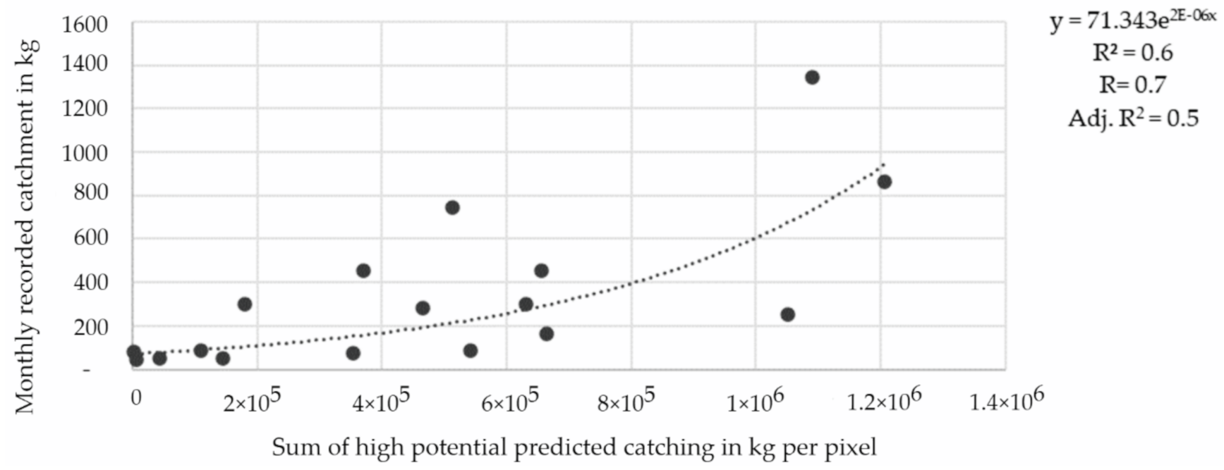
3.4. Lobster Harvest Potential and Relationship with Catch Data in Palabuhanratu Bay

The regression model was implemented using imagery from other months to determine the relationship between the recorded value and the sum of the predicted catch in kilograms per pixel. Due to the unavailability of a monthly point catch, the recorded monthly data on lobsters purchased from fishermen by a collector in the Palabuhanratu fish market were used. It was assumed that the result of the model prediction should be followed with the recorded catch data. This study only included satellite imagery that had cloud cover below 50% of the trendline. An exponential trendline was used to find the R, R², and adj R² values, which were 0.753, 0.567, and 0.538, respectively (Figure 7). This means that the recorded catch values agreed well with the predicted catch values, and that the model could consequently be implemented in other months. Exponential trendlines are curved lines that are useful when data values are increasing or decreasing at a growing rate [51]. The good agreement between the model and actual catch data was not directly followed by the same value. The sum of the predicted catch in the high-potential harvest area showed a much higher value than the actual recorded catch. This is not unexpected, as the estimated potential should be higher than the fishermen’s capability to catch lobsters.

The distribution of potential lobster harvest grounds from March 2015 to November 2016 can be seen in Figure 8. The spatial distribution of lobster harvest potential was divided into three classes: low, moderate, and high potential. The range of values for each class is shown in

Table 3. Classification of predicted catches.

Class	Predicted Catches in kg/pixel
Low	0–2.799
Moderate	2.800–3.433
High	3.434–10.791

.

Figure 8 shows the distribution of potential lobster harvests during 2016–2017. The areas with the highest potential for lobster harvests in March 2015 were in the northwest and southeastern parts of the bay, around the waters of Cisolok and Simpenan, with a potential area of 54 km². In April 2015, the area with the highest potential for lobster harvests was 4 km², which had decreased from the previous month and had moved further out to sea. Furthermore, in May 2015, the area with the highest potential for lobster harvests was 11 km², which had moved to the southwest of the bay. The area of highest lobster harvest potential in June 2015 increased to 128 km² and was mostly located in the deeper areas of the sea. However, in the waters of Ciemas, Simpenan, and Palabuhanratu, the potential areas were located around the coast. In July 2015, the area with the highest lobster harvest potential was in the deeper seas of the Ciemas and Bayah waters, with an area of 35 km². The highest potential area for lobster harvests in August 2015 then moved to the northwest of the bay, with an area of 46 km². In September 2015, the area with the highest potential for lobster harvests tended to be on the coast in the Ciemas and Simpenan waters, with an area of 62 km². The area with the highest potential for lobster harvests in October 2015 remained around the coast of Palabuhanratu and Simpenan, but had shrunk to 36 km². Then, in November 2015, the area with the highest potential for lobster harvests was around the coast of Simpenan and close to the deeper sea in the west of the bay, with an area of 25 km².

The beginning of 2016 was preceded by the formation of areas with the highest potential for lobster harvests from the north to the west of the bay, in the waters of Cisolok and Cikakak and along the coast of Simpenan, with an area of 61 km². In February 2016, the area with the highest potential for lobster harvests moved to the middle of the bay, with an area of 92 km². In April 2016, the area with the highest potential for lobster harvests was around the coast of Cisolok and Cikakak, with an area of 14 km². Then, in May 2016, the area with the highest potential for lobster harvests moved toward the deeper sea in Bayah, with an area of 11 km². In June and July, the areas with the highest potential for lobster harvests were very small and were located in the east of the bay, with areas of 2 and 3 km², respectively, which was because most of the imagery was obscured by clouds. The areas with the highest potential for lobster harvests in September 2016 were on the Cikakak and Palabuhanratu coasts and slightly spread out into the deeper sea of Cikakak, with an area of 18 km². Then, in November 2016, the highest potential for lobster harvests increasingly moved toward the deep sea, with an area of 11 km². By contrast, March and August 2016 did not have high lobster harvest potential, suggesting that lobster fishing is not recommended during these months.

4. Discussion

In recent years, the topic of lobster harvesting has become a sensitive issue in Indonesia, particularly regarding the commercialization of juvenile lobsters [52]. Even though Indonesia’s waters have large potential for harvests of mature lobsters, exportation is still dominated by juveniles with less economic value and at greater risk of stock collapse. Fishermen likely catch the juveniles because they are easier to catch than mature lobsters. However, the over-exploitation of juveniles will cause a loss in terms of future lobster resources. The Indonesian government is currently formulating regulations for the harvest of juvenile and mature lobsters.

The recommended map of potential harvest areas for marine resources (i.e., pelagic fishes and tuna) has already been widely used by Indonesian fishermen and has been successful in improving the numbers caught [53]. However, in terms of implementation, local authorities’ involvement in disseminating this information has played a large role [54,55]. This study proposed a predictive map of lobster harvest grounds that will help fishermen increase their probability of catching mature lobsters in open-water areas. If the number of successful mature lobster catches increases, this should be followed by increased interest from fishermen in catching mature rather than juvenile lobsters. This is because the price of a mature lobster is much higher than that of a juvenile lobster. Improving the number of mature lobsters caught might be a solution to the problem of juvenile lobster exploitation in Indonesia.

Based on our study, the potential lobster harvest grounds are mostly on the coast of the Simpenan waters, which are known to have corals that are preferred by lobsters for their habitat [31]. This is reinforced by interviews with fishermen in Palabuhanratu Bay, which have shown that lobster catch locations are mostly found around Simpenan. From Figure 8, in the month that was classified as having a lower potential, the area with a high potential for lobster harvests was larger and toward the deeper sea. This was because, in that month, lobsters tend to move into deeper waters at a depth of approximately 37 to 55 m to spawn [56], which shifted the lobster harvest areas to the deeper sea. The area with the highest potential was seen in June 2015, with an area of 128 km².

Throughout the observations, Landsat-8 images of Palabuhanratu Bay could not always be collected. This was because of limitations of the long temporal resolution (revisit time of 16 days) and on the availability of cloud-free data. An alternative is the Sentinel-2 (S2) image series, which provides dense observations (revisit time of 5 days under S2A and S2B satellites) [57]. However, the S2 images do not have a thermal band, which is used for extracting the SST value. As this study found that SST and salinity have a strong correlation, they play an important role in modeling lobster harvest areas. This fact correlates favorably with studies by Mahima et al. [11], Pradhan et al. [13], and Zhao et al. [12] and also further supports the effect of climate change on marine food chains. Moreover, SST and salinity were found to be important in the modeling harvest potential for other marine resources as well, such as tuna [58] and pelagic fish [59].

This study found that the fluctuation in lobster catches could be determined by optimal and ideal oceanographic conditions using chlorophyll-a, salinity, TSS, SSTs, distance from the coastline, and other oceanographic parameters. This study provided a new understanding of the relationship of those parameters to lobster harvest grounds. Given that our findings were based only on four species of lobster and a small number of samples, the results from such analyses should consequently be treated with considerable caution. In future studies, we suggest analyzing the spatial model for each species separately, as well as using more samples and more timeseries datasets on lobster catches. Furthermore, other physical oceanographic parameters, such as rainfall, ocean currents, and tides, can be used to develop better models.

5. Conclusions

The variables chlorophyll-a, salinity, TSSs, SST, and distance from the coastline simultaneously had a significant effect on lobster catches. From these five variables, the lobster harvest prediction model potential was obtained using the multiple linear regression method, namely Y = −60.7232 − (0.374 × Chl-a) + (0.554 × Salinity) + (0.052 × TSS) + (1.601 × SST) − (0.001 × Distance). This model had an adjusted R² value of 0.708; therefore, it could be used to predict lobster harvest potential at different times. The sea surface temperature, followed by salinity, were the variables most valuable to the prediction model. It should be noted that the model was built on the basis of the local algorithm of Landsat-8-derived oceanographic parameters, so the presented results are not applicable to global predictions, as the algorithm we used might not fit with other regional oceanographic characteristics. However, the proposed prediction model followed the monthly recorded harvest in an exponential manner. Overall, the predicted potential lobster harvest grounds were generally located off the coast of Simpenan and the highest recorded potential area was 128 km² in June 2015.

References

1. Moosa, M.K.; Aswandy, I. Udang Karang (Panulirus spp.) Dari Perairan Indonesia; Lembaga Ilmu Pengetahuan Indonesia: Jakarta, Indonesia, 1984. [Google Scholar]
2. Fauzi, M.; Prasetyo, A.P.; Hargiyatno, I.T.; Satria, F.; Utama, A.A. Hubungan panjang-berat dan faktor kondisi lobster batu (Panulirus penicillatus) di perairan selatan Gunung Kidul dan Pacitan. Bawal 2013, 5, 97–102. [Google Scholar]
3. Fadila, I. Larangan tangkap lobster: Ekspor lobster bisa meningkat signifikan. 2015. Available online: https://ekonomi.bisnis.com/read/20150129/99/396347/larangan-tangkap-lobster-ekspor-lobster-bisa-meningkat-signifikan (accessed on 24 December 2019).
4. Khikmawati, L.T.; Martasuganda, S.; Sondita, M.F.A. The body of lobster catches in Palabuhanratu than the applicable regulatory. J. Ilmu Teknol. Kelaut. Trop. 2017, 9, 507–520. [Google Scholar] [CrossRef] [Green Version]
5. Sudrajat, S.M.N.I.; Rosyid, A.; Bambang, A.N. Analisis teknis dan finansial usaha penangkapan ikan layur (Trichiurus sp) dengan alat tangkap pancing ulur (handline) di pelabuhan perikanan nusantara Palabuhanratu Sukabumi. J. Fish. Resour. Util. Manag. Technol. 2014, 3, 141–149. [Google Scholar]
6. Hutabarat, S.; Evans, S. Pengantar Oseanografi; UI-Press: Jakarta, Indonesian, 1984. [Google Scholar]
7. Cooke-Panton, K. An Analysis of Puerulus Settlement of the Caribbean Spiny Lobster (Panulirus Argus) Stock in Jamaica with Practical Management Recommendations; United Nations University: Iceland, 2014; Available online: https://www.grocentre.is/static/gro/publication/306/document/kim14prf.pdf (accessed on 24 December 2019).
8. Chiswell, S.M.; Booth, J.D. Sources and sinks of larval settlement in Jasus edwardsii around New Zealand: Where do larvae come from and where do they go? Mar. Ecol. Prog. Ser. 2008, 354, 201–217. [Google Scholar] [CrossRef]
9. Williams, K.C.; Jones, C.; van Hung, L.; Tuan, L.A.; Hoang, D.H.; Huong, L.L.; Thuy, N.B.; Pahlevi, R.S.; Priyambodo, B. Sustainable Tropical Spiny Lobster Aquaculture in Vietnam and Australia (and Extension to Indonesia); ACIAR: Canberra, Australia, 2010.
10. Thangaraja, R.; Radhakrishnan, E.V. Fishery and ecology of the spiny lobster Panulirus homarus (Linnaeus, 1758) at Khadiyapatanam in the southwest coast of India. J. Mar. Biol. Assoc. India 2012, 54, 69–79. [Google Scholar] [CrossRef]
11. Jaini, M.; Wahle, R.A.; Thomas, A.C.; Weatherbee, R. Spatial surface temperature correlates of American lobster (Homarus americanus) settlement in the Gulf of Maine and southern New England shelf. Bull. Mar. Sci. 2018, 94, 737–751. [Google Scholar] [CrossRef]
12. Zhao, X.; Ding, P.; Pang, J. Implications of ocean bottom temperatures on the catch ability of American lobster. In Proceedings of the E3S Web of Conferences, EDP Sciences, Wuhan, China, 14–16 December 2018; Volume 79. [Google Scholar]
13. Pradhan, S.K.; Iburahim, S.A.; Nakhawa, A.D.; Shenoy, L. Effect of environmental parameters on estuarine lobster and crab fishery and its management in thane estuary, Maharashtra. J. Entomol. Zool. Stud. 2019, 7, 102–104. [Google Scholar]
14. Beni, Z.; Wardiatno, Y. Biological aspect of double-spined rock lobster (Panulirus penicillatus) in Wonogiri Regency waters, Central Java, Indonesia. IOP Conf. Ser. Earth Environ. Sci. 2020, 420. [Google Scholar] [CrossRef]
15. Butler, M.J. Collecting and processing lobsters. J. Crustac. Biol. 2017, 37, 340–346. [Google Scholar] [CrossRef]
16. NF, Z.S.; Rivani, A.; Puspitasari, B.; Ikhwansyah, F.; Maulidyah, F.; Dwi D, R.; Eka P, S.; Widyatmanti, W. Marine environmental suitability mapping for lobster sea-cage culture in east Lombok using remote sensing data and GIS approaches. Aquac. Indones. 2017, 17, 60. [Google Scholar] [CrossRef] [Green Version]
17. Aiken, D.E.; Waddy, S.L. Environmental influence on recruitment of the American lobster, Homarus americanus: A perspective. Can. J. Fish. Aquat. Sci. 1986, 43, 2258–2270. [Google Scholar] [CrossRef]
18. Mercaldo-Allen, R.; Kuropat, C.A. Review of American Lobster (Homarus Americanus) Habitat Requirements and Responses to Contaminant Exposures; U.S. Department of Commerce, National Oceanic and Atmospheric Administration: Washington, DC, USA, 1994.
19. Rhodes, C.J.; Henrys, P.; Siriwardena, G.M.; Whittingham, M.J.; Norton, L.R. The relative value of field survey and remote sensing for biodiversity assessment. Methods Ecol. Evol. 2015, 6, 772–781. [Google Scholar] [CrossRef]
20. USGS. Using the USGS Landsat Level-1 Data Product. Available online: https://www.usgs.gov/land-resources/nli/landsat/using-usgs-landsat-level-1-data-product (accessed on 24 December 2019).
21. De Lara, V.C.-F.; Butler, M.; Hernández-Vázquez, S.; Del Próo, S.G.; Serviere-Zaragoza, E. Determination of preferred habitats of early benthic juvenile California spiny lobster, Panulirus interruptus, on the Pacific coast of Baja California Sur, Mexico. Mar. Freshw. Res. 2005, 56, 1037–1045. [Google Scholar] [CrossRef] [Green Version]
22. Rios-Lara, V.; Salas, S.; Javier, B.P.; Ayora, P.I. Distribution patterns of spiny lobster (Panulirus argus) at Alacranes Reef, Yucatan: Spatial analysis and inference of preferential habitat. Fish. Res. 2007, 87, 35–45. [Google Scholar] [CrossRef]
23. Whomersley, P.; Van der Molen, J.; Holt, D.; Trundle, C.; Clark, S.; Fletcher, D. Modeling the dispersal of spiny lobster (Palinurus elephas) larvae: Implications for future fisheries management and conservation measures. Front. Mar. Sci. 2018, 5, 1–16. [Google Scholar] [CrossRef] [Green Version]
24. Setyanto, A.; Soemarno; Wiadnya, D.G.R.; Prayogo, C. Biodiversity of lobster larvae (Panulirus spp.) from the Indonesian Eastern Indian Ocean. IOP Conf. Ser. Earth Environ. Sci. 2019, 370. [Google Scholar] [CrossRef]
25. Wahyudin, R.; Hakim, A.; Qonita, Y.; Boer, M.; Farajallah, A.; Mashar, A.; Wardiatno, Y. Lobster diversity of Palabuhanratu Bay, South Java, Indonesia with new distribution record of Panulirus ornatus, P. polyphagus and Parribacus antarcticus. AACL Bioflux 2017, 10, 308–327. [Google Scholar]
26. Damora, A.; Adrianto, L.; Wardiatno, Y.; Suman, A. Dynamic spatial allocation of scalloped spiny lobster (Panulirus homarus) in the coast of Gunungkidul, Indonesia. IOP Conf. Ser. Earth Environ. Sci. 2019, 348, 012113. [Google Scholar] [CrossRef] [Green Version]
27. Pranata, B.; Sabariah, V. Suhaemi Aspek biologi dan pemetaan daerah penangkapan lobster (Panulirus spp) di perairan Kampung Akudiomi Distrik Yaur Kabupaten Nabire. Sumber Daya Akuatik Indopasifik 2017, 1, 1–14. [Google Scholar]
28. Nurfiarini, A.; Wijaya, D.; Satria, F.; Kartamihardja, E.S. Pendekatan sosial-ekologi untuk penilaian kesesuaian lokasi restocking lobster pasir Panulirus homarus (Linnaeus, 1758) pada beberapa perairan di Indonesia. J. Penelit. Perikan. Indones. 2016, 22, 123–138. [Google Scholar]
29. Erlania, E.; Radiarta, I.N.; Sugama, K. Dinamika kelimpahan benih lobster (Panulirus spp.) Di perairan Teluk Gerupuk, Nusa Tenggara Barat: Tantangan pengembangan teknologi budidaya lobster. J. Ris. Akuakultur 2014, 9, 475. [Google Scholar] [CrossRef] [Green Version]
30. Khikmawati, L.T. Modifikasi Hang-in Ratio Jaring Insang Dasar dan Pengaruhnya Terhadap Karakteristik Hasil Tangkapan di Palabuhanratu Jawa Barat; Institut Pertanian Bogor: Bogor, Indonesia, 2017. [Google Scholar]
31. WWF Indonesia. Perikanan Lobster Laut, 1st ed.; WWF Indonesia: Jakarta, Indonesian, 2015; ISBN 9789791461689. [Google Scholar]
32. Kadafi, M.; Widaningroem, R. Biological aspects and maximum sustainable yield of spiny lobster (Panulirus spp.) in Ayah coastal waters Kebumen Regency. J. Fish. Sci. 2006, 8, 108–117. [Google Scholar]
33. USGS. Landsat 8 Surface Reflectance Code (LASRC) product guide (No. LSDS-1368 Version 2.0); USGS: Reston, VA, USA, 2019.
34. Gorelick, N.; Hancher, M.; Dixon, M.; Ilyushchenko, S.; Thau, D.; Moore, R. Google Earth Engine: Planetary-scale geospatial analysis for everyone. Remote Sens. Environ. 2017, 202, 18–27. [Google Scholar] [CrossRef]
35. Firdaus, F. Persebaran Fitoplankton di Estuari Cimandiri Sebelum dan Sesudah Adanya PLTU Pelabuhanratu; Universitas Indonesia: Jawa Barat, Indonesia, 2017. [Google Scholar]
36. Kaffah, S.; Supriatna; Damayanti, A. Cilamaya estuary zonation based on sea surface salinity with 2 Sentinel-2A satellite imagery. IOP Conf. Ser. Earth Environ. Sci. 2020, 481, 481. [Google Scholar] [CrossRef]
37. Budhiman, S.; Hobma, T.W.; Vekerdy, Z. Remote sensing for mapping TSM concentration in Mahakam Delta: An analytical approach. In Proceedings of the 13th OMISAR Workshop on Validation and Application of Satellite Data for Marine Resources Conservation, Bali, Indonézia, 5–9 October 2004. [Google Scholar]
38. Syariz, M.A.; Jaelani, L.M.; Subehi, L.; Pamungkas, A. Retrieval of sea surface temperature over Poteran Island water of Indonesia with Landsat 8 TIRS image: A preliminary algorithm. Int. Arch. Photogramm. Remote Sens. Spat. Inf. Sci. 2015, XL-2/W4, 87–90. [Google Scholar] [CrossRef] [Green Version]
39. Mukhtar, M.K.; Manessa, M.D.M.; Supriatna, S. The validation of water quality parameter algorithm using Landsat 8 and Sentinel-2 image in Palabuhanratu Bay. In Proceedings of the LEAF Conference (preprint), Depok, Indonesia, 6–7 November 2020. [Google Scholar]
40. Jenks, G. The Data Model Concept in Statistical Mapping. International Yearbook of Cartography 7: George Philip. 1967, pp. 186–190. Available online: https://support.esri.com/en/technical-article/000006743 (accessed on 24 December 2019).
41. Kutner, M.H.; Nachtsheim, C.J.; Neter, J. Applied Linear Statistical Models, 4th ed.; Gordon, B., Ed.; McGraw-Hill/Irwin: New York, NY, USA, 2004; Volume 29, ISBN 0072386886. [Google Scholar]
42. Kohavi, R. A study of cross-validation and bootstrap for accuracy estimation and model selection. Int. Jt. Conf. Artif. Intell. 1995, 2, 1137–1143. [Google Scholar]
43. Chai, T.; Draxler, R.R. Root mean square error (RMSE) or mean absolute error (MAE)? -Arguments against avoiding RMSE in the literature. Geosci. Model Dev. 2014, 7, 1247–1250. [Google Scholar] [CrossRef] [Green Version]
44. Lewis-Beck, M.; Bryman, A.; Futing Liao, T. R-squared. SAGE Encycl. Soc. Sci. Res. Methods 2012, 1187–1190. [Google Scholar] [CrossRef]
45. Bolar, K. Interactive Document for Working with Basic Statistical Analysis; [R package stat version 0.1.0]. Available online: https://cran.r-project.org/web/packages/STAT/index.html (accessed on 24 December 2019).
46. Hijmans, R.J.; van Etter, J.; Cheng, J.; Mattiuzzi, M.; Summer, M.; Greenberg, J.A.; Lamigueiro, O.P.; Bevan, A.; Racine, E.B.; Shortridge, A.; et al. Geographic Data Analysis and Modeling; [R package raster version 2.9-5]. Available online: https://CRAN.R-project.org/package=raster (accessed on 24 December 2019).
47. Bivand, R.; Keitt, T.; Rowlingson, B.; Pebesma, E.; Sumner, M.; Hijmans, R.; Baston, D.; Rouault, E.; Warmerdam, F.; Ooms, J.; et al. Bindings for the “Geospatial” Data Abstraction Library; [R package rgdal version 1.5-23]. Available online: http://rgdal.r-forge.r-project.org/ (accessed on 24 December 2019).
48. Lind, D.A.; Marchal, W.G.; Wathen, S.A. Statistical Techniques in Business & Economics; McGraw Hill: New York, NY, USA, 2015; ISBN 9780073401805. [Google Scholar]
49. Hair, J.F.; Anderson, R.; Tatham, R.; Black, W.C. Multivariate Data Analysis, 3rd ed.; Macmillan: New York, NY, USA, 1995. [Google Scholar]
50. Kuhn, M. Building predictive models in R using the caret Package; [R package caret version 3.45]. J. Stat. Softw. 2008, 28, 1–26. [Google Scholar] [CrossRef] [Green Version]
51. Microsoft. Choosing the Best Trendline for Your Data. Available online: https://support.microsoft.com/en-us/office/choosing-the-best-trendline-for-your-data-1bb3c9e7-0280-45b5-9ab0-d0c93161daa8 (accessed on 25 January 2021).
52. Gokkon, B. Indonesia’s Lobster Export Safeguards Won’t End Smuggling, Scientists Warn. Available online: https://news.mongabay.com/2020/06/indonesias-lobster-export-safeguards-wont-end-smuggling-scientists-warn/ (accessed on 24 December 2020).
53. Atmajaya, O.D.D.; Simbolon, D.; Wiryawan, B. Persepsi pemanfaatan peta daerah penangkapan ikan di perairan Sendang Biru Malang. ALBACORE J. Penelit. Perikan. Laut 2018, 1, 163–170. [Google Scholar] [CrossRef]
54. Avianti, D. Efektivitas Pemanfaatan Peta Prakiraan Daerah Penangkapan Ikan Oleh Nelayan Gillnet di Pelabuhan Perikanan Samudera Cilacap; IPB University: Bogor, Indonesian, 2019. [Google Scholar]
55. Huwaida, H. Evaluasi Pemanfaatan Peta Prakiraan Daerah Penangkapan Ikan Pada Perikanan Long Line di Pelabuhan Perikanan Samudera CILACAP; IPB University: Bogor, Indonesian, 2019. [Google Scholar]
56. Boesono, H.; Anggoro, S.; Bambang, A.N. Laju tangkap dan analisis usaha penangkapan lobster (Panulirus sp) dengan jaring lobster (gillnet monofilament) di perairan kabupaten Kebumen. J. Saintek Perikan. 2011, 7, 77–87. [Google Scholar] [CrossRef]
57. ESA. Sentinel-2—Missions—Sentinel. Available online: https://sentinel.esa.int/web/sentinel/missions/sentinel-2 (accessed on 24 February 2021).
58. Cornic, M.; Rooker, J.R. Influence of oceanographic conditions on the distribution and abundance of blackfin tuna (Thunnus atlanticus) larvae in the Gulf of Mexico. Fish. Res. 2018, 201, 1–10. [Google Scholar] [CrossRef]
59. Oozeki, Y.; Takasuka, A.; Barange, M. Characterizing Spawning Habitats of Japanese Sardine (Sardinops melanostictus), Japanese Anchovy (Engraulis japonicus), and Pacific Round Herring (Etrumeus teres) in the Northwestern Pacific; California Cooperative Oceanic Fisheries Investigation Report 48; Yokohama: Tokyo, Japan, 2007. [Google Scholar]
Figure 1. Research location. Red dots show the collected lobster catch points.
Fishes 06 00016 g001
Figure 2. Lobster type in Palabuhanratu Bay [30].
Fishes 06 00016 g002
Figure 3. Research methodology.
Fishes 06 00016 g003
Figure 4. The harvest weights of lobsters under different ranges of environmental conditions.
Fishes 06 00016 g004
Figure 5. Correlations (R) between variables. A value that is close to ±1 has a high correlation, and vice versa.
Fishes 06 00016 g005
Figure 6. Model cross-validation test. The model improves if the RMSE value is close to 0 and the R2 is close to 1.
Fishes 06 00016 g006
Figure 7. Relationship between predicted and observed catches (kg).
Fishes 06 00016 g007
Figure 8. Potential lobster harvest grounds. Several months (i.e., January–February 2015, January 2016 and December 2016) did not have available images due to high cloud coverage.
Fishes 06 00016 g008