
Article

Revealing Seasonal Environmental Associations and Spatial Heterogeneity of Pacific Yellowfin Tuna CPUE Using an Interpretable Neural Network Framework

1
College of Marine Living Resources Sciences and Management, Shanghai Ocean University, Shanghai 201306, China
2
National Engineering Research Center for Oceanic Fisheries, Shanghai Ocean University, Shanghai 201306, China
3
Key Laboratory of Sustainable Exploitation of Oceanic Fisheries Resources, Ministry of Education, Shanghai 201306, China
4
Key Laboratory of Oceanic Fisheries Exploration, Ministry of Agriculture and Rural Affairs, Shanghai 201306, China
5
Scientific Observing and Experimental Station of Oceanic Fishery Resources, Ministry of Agriculture and Rural Affairs, Shanghai 201306, China
*
Author to whom correspondence should be addressed.
Fishes 2026, 11(9), 539; https://doi.org/10.3390/fishes11090539 (registering DOI)
Submission received: 7 August 2026 / Revised: 3 September 2026 / Accepted: 10 September 2026 / Published: 13 September 2026
(This article belongs to the Section Biology and Ecology)

Abstract

Understanding the spatial distribution patterns of pelagic species such as yellowfin tuna (Thunnus albacares) is essential for ecosystem-based fisheries management. However, characterizing CPUE–environment relationships remain challenging because these relationships may be nonlinear and spatially heterogeneous across large oceanic regions. To address these challenges, we developed an interpretable spatial modeling framework, geographically neural network weighted regression integrated with GeoShapley analysis (GNNWR-GeoShapley), which combines the nonlinear learning capability of neural networks with spatially explicit characterization and interpretation of model relationships. Using Pacific longline fishery data and multi-source environmental variables from 2004 to 2023, we constructed quarterly models of CPUE–environment relationships and compared the performance of GNNWR with Generalized additive model (GAM), geographically weighted regression (GWR), graph neural network (GNN) models, and Geographical Random Forest (GRF). The results demonstrated that GNNWR showed the best overall performance across seasons, effectively capturing nonlinear relationships and spatial heterogeneity in yellowfin tuna nominal CPUE. GeoShapley analysis further revealed that sea surface and subsurface (150 m) temperature and salinity were among the most important environmental variables associated with nominal CPUE variations. Nonlinear response patterns indicated that SST values above approximately 25 °C and T150 values above approximately 19 °C were associated with positive model contributions, whereas higher salinity values (>35) exhibited negative contributions. Moreover, spatial effects represented by the geographical location variable (GEO) and their interactions with environmental variables revealed pronounced spatial heterogeneity, with the contribution patterns of environmental factors varying across seasons and regions. This study provides an interpretable spatial modeling framework for characterizing complex species–environment relationships and offers new insights into the spatial variability of Pacific yellowfin tuna nominal CPUE for fisheries oceanography and sustainable resource management.
Key Contribution: This study develops an interpretable spatial modeling framework by integrating GNNWR with GeoShapley to improve the interpretation of Pacific yellowfin tuna nominal CPUE patterns. The proposed framework provides new insights into spatially heterogeneous CPUE–environment associations by simultaneously capturing nonlinear relationships, spatially varying relationships, and environmental contributions across seasons.

1. Introduction

Yellowfin tuna (Thunnus albacares) is broadly distributed across tropical and subtropical oceans [1]. It represents one of the major target species of global longline fisheries. Their stock status is critical to global fishery economics and food security [2]. The Pacific Ocean accounted for 68% of the global yellowfin catch in 2024 [3], making it the most important fishing ground. The spatial distributions of yellowfin tuna are closely related to marine environmental factors, which shape their foraging behavior, migration routes, and aggregation characteristics [4]. However, the Pacific Ocean is vast, with a longitudinal span of over 15,000 km. It encompasses diverse marine environmental systems such as the Western Pacific Warm Pool, the equatorial cold tongue, and the equatorial upwelling zone, exhibiting significant spatial heterogeneity and environmental complexity [5,6]. These complex environmental dynamics pose significant challenges to characterizing the spatially heterogeneous and nonlinear relationships between the spatial distribution of pelagic fishes and environmental factors, thereby complicating the implementation of effective fisheries management.
Extensive research has investigated the environmental associations underlying tuna distribution patterns. Early statistical methods capture nonlinear environmental effects well [7,8]; however, being global models, they fail to resolve spatial heterogeneity. The subsequent application of Geographically Weighted Regression (GWR) successfully resolved the spatial heterogeneity in resource–environment responses [9,10]. But these methods usually rely on the assumption of local stationarity and are difficult to effectively depict strong nonlinear relationships in large-scale complex marine environments. Recently, machine learning algorithms such as Random Forests [11], Gradient Boosting Trees [12], Geographical Random Forests [5], and Neural Networks [13] have been widely applied in habitat modeling. Although these methods can effectively capture complex nonlinear relationships, many models lack explicit representations of spatial structures, limiting their ability to interpret spatially varying relationships between environmental factors and species distributions [14].
To address these issues, the Geographically Neural Network Weighted Regression (GNNWR) model integrates the ability of GWR to represent spatial heterogeneity with the powerful nonlinear learning capability of neural networks [15]. GNNWR has demonstrated potential for capturing both spatial heterogeneity and nonlinear relationships in urban and environmental studies [16,17]. This capability is particularly relevant to pelagic species, whose relationships with environmental conditions can vary substantially across large and heterogeneous oceanic regions. Therefore, we attempted to apply GNNWR to characterize the complex spatially heterogeneous and nonlinear relationships between nominal CPUE of yellowfin tuna in the Pacific Ocean and environmental factors. Furthermore, to enhance model interpretability, we introduce the recently proposed GeoShapley method [18]. By explicitly incorporating spatial information into the explanation framework, GeoShapley enables the quantification of complex interactions between geographical locations and environmental variables, allowing for improved interpretation of spatial heterogeneity in species–environment relationships.
In this study, we combined the GNNWR model with GeoShapley to investigate the environmental associations with yellowfin tuna nominal CPUE patterns in the Pacific Ocean. We integrated 20 years of longline fishery data (from 2004 to 2023) and marine environmental data to construct the models. We aimed to address the primary scientific question of how nonlinear and spatially heterogeneous CPUE–environment relationships vary across the Pacific and seasons, and how these relationships can be effectively interpreted. By integrating GNNWR with GeoShapley, we further sought to address the limitation of existing spatial machine-learning approaches that may capture nonlinear patterns but provide limited insight into how environmental effects vary spatially and interact with geographic context. Our primary objectives are: (1) to construct a GNNWR model for Pacific yellowfin tuna nominal CPUE and evaluate its performance by comparing it with traditional Generalized additive model (GAM), GWR, Graph Neural Network (GNN), and GRF models; (2) to interpret the GNNWR model results using the GeoShapley method, thereby characterizing the contributions of environmental variables and their seasonal and spatial variations; (3) to provide a new perspective for understanding the large-scale ecological adaptation strategies of highly migratory species in complex pelagic environments, offering scientific information relevant to fisheries oceanography and regionally differentiated spatial management in the Pacific.

2. Materials and Methods

2.1. Data Sources

2.1.1. Fisheries Data

We extracted open-access longline records (2004–2024) from the Western and Central Pacific Fisheries Commission (WCPFC) and the Inter-American Tropical Tuna Commission (IATTC) repositories for a vast Pacific domain (35° S–35° N, 130° E–80° W). The original fisheries data have a spatial resolution of 5° × 5° and a monthly temporal resolution. And the dataset includes operational time, latitude and longitude of the fishing operations, fishing effort (number of hooks), as well as the catch in weight and catch in numbers of yellowfin tuna.

2.1.2. Environmental Data

As a warm-water pelagic species, the distribution, migration, and aggregation behaviors of yellowfin tuna are significantly regulated by marine environmental factors [19]. In this study, we initially selected 21 environmental variables—encompassing thermohaline, hydrodynamic, and biogeochemical indicators—that potentially affect the spatial distribution of this species. Detailed information regarding these variables, including their specific depth layers and data sources, is summarized in Table 1.

2.2. Data Processing

2.2.1. Data Preparation

Because the fisheries response variable was available at a spatial resolution of 5° × 5°, all environmental variables were aggregated to the same analytical grid to ensure spatial consistency between the factors and CPUE observations. The 5° × 5° resolution was therefore determined by the spatial support of the available longline fishery data rather than being selected as an intrinsically optimal ecological resolution. Although several environmental datasets were originally available at finer spatial resolutions, disaggregating the fisheries data to finer grids would not provide additional information on the response variable and could introduce artificial spatial structure or pseudo-replication. The spatial aggregation allows the characterization of broad-scale environmental gradients associated with major Pacific oceanographic systems, such as the Western Pacific Warm Pool and the equatorial cold tongue, while inevitably smoothing sub-grid environmental variability, including thermal fronts, mesoscale eddies, and localized upwelling processes. Therefore, the present analysis is intended to characterize broad-scale seasonal spatial patterns and spatially heterogeneous environmental associations with yellowfin tuna nominal CPUE rather than fine-scale habitat features or mesoscale ecological processes.
Temporally, the monthly data of both fishery and environmental variables were aggregated into quarterly intervals: Q1 (January–March), Q2 (April–June), Q3 (July–September), and Q4 (October–December). This temporal aggregation was used to characterize seasonal environmental conditions and reduce short-term variability in both the fishery and environmental observations. Furthermore, because the model constructs spatial structures based on spatial proximity, data points located at the peripheral boundaries of the study area or adjacent to landmasses were excluded during preprocessing to reduce potential edge effects and preserve spatial continuity. To further evaluate the temporal transferability of the trained GNNWR model, independent-year validation was conducted using the 2024 fishery and environmental data. The 2024 data were not included in model training and were used solely for an independent assessment of model performance under an unseen year.

2.2.2. CPUE Calculation

Catch per unit effort (CPUE) is commonly used as an indicator of fishing efficiency and a proxy for relative abundance in fisheries studies [20,21]. In this study, we calculated the 20-year average nominal CPUE for yellowfin tuna within each 5° × 5° grid cell for the four quarters. The nominal CPUE was calculated as follows:
CPUE i , j = Catch i , j Effort i , j × 1000
C P U E i , j , C a t c h i , j and E f f o r t i , j represent the CPUE, the total number of fish caught, and the total number of hooks deployed within the grid cell at longitude i and latitude j.
Due to the lack of complete operational information, such as hook depth, bait type, vessel-specific fishing strategy, and targeting behavior, a fully standardized CPUE was not available for this study. Nominal CPUE integrates both ecological signals from yellowfin tuna distribution and variation arising from fishing practices and catchability. Differences in gear configuration and targeting behavior may affect observed CPUE independently of environmental conditions, and because fishing practices are not uniformly distributed in space or time, they may confound or contribute to the estimated CPUE–environment relationships. The estimated environmental associations may thus partly reflect unobserved operational variation and should be interpreted with appropriate caution.
To mitigate short-term variability associated with individual fishing operations, we applied 20-year spatial averaging and quarterly temporal aggregation. These procedures emphasize relatively persistent spatial patterns in CPUE and reduce the influence of transient operational effects. Accordingly, the modeled relationships are interpreted as associations between environmental conditions and observed nominal CPUE patterns, rather than as direct measures of population abundance or as causal effects on yellowfin tuna stocks.

2.2.3. Environmental Factor Selection

To select the optimal environmental factors, we first conducted a Spearman correlation analysis quarterly (Figure S1) to evaluate the relationships between the 21 initial environmental variables and nominal CPUE. To reduce multicollinearity, we subsequently applied the Variance Inflation Factor (VIF) test. Variables exhibiting high collinearity were progressively eliminated based on their correlation strength, VIF values, and environmental relevance. Ultimately, eight environmental variables were retained: SST, T150, SSS, S150, MLD, DO, NPP, and SLA (Table 2). The retained variables showed acceptable levels of multicollinearity under the adopted screening criterion and were used for subsequent model training. Detailed procedures regarding the variable selection process are provided in Text S1 of the Supplementary Information.

2.3. GNNWR-Geoshapley Model

Traditional spatial statistical models, such as GWR, effectively address spatial non-stationarity by allowing parameters to vary over space; however, they often struggle to capture complex nonlinear relationships. Conversely, deep learning models like Graph Neural Networks (GNNs) excel at learning complex spatial dependencies through message-passing mechanisms and attention architectures. Yet they lack the explicit geographic weighting mechanisms required for intuitive spatial interpretation.
To overcome these respective limitations, we employed the GNNWR model. GNNWR seamlessly integrates the spatial weighting principles of GWR with the robust nonlinear fitting capabilities of neural networks [15]. The core of GNNWR lies in its neural network module, which utilizes a Spatially Weighted Neural Network (SWNN) to represent the non-stationary weight matrix, thereby enabling local parameter estimation. Given its proven superiority in modeling complex spatial phenomena [16,22], we applied GNNWR to investigate the environmental associations of yellowfin tuna nominal CPUE in the Pacific Ocean. The model structure is formulated as follows:
CPUE i   =   w 0 u i , v i × β 0 + k = 1 p w k u i , v i × β k x ik + ε i   i = 1 , 2 , , n
where w k u i , v i represents the spatial weight of the k-th independent variable for sample i at location u i , v i , a n d   β = β 0 , β 1 , , β k are the coefficients of the Ordinary Least Squares Regression (OLR), reflecting the average state of the Pacific yellowfin tuna nominal CPUE. The Ordinary Least Squares estimate of β is expressed as follows:
β ^   =   ( X T X ) 1 X T CPUE
The predicted value of CPUE is calculated as follows:
C PU ^ E i   =   k = 0 8 w ik × β ^ k ( OLR ) × x ik = x i T W i X T X 1 X T CPUE
where W i is the spatial weight matrix. The GNNWR approach employs a Spatial Weight Neural Network (SWNN) to dynamically determine distance-based spatial weights. By utilizing the distances between an evaluation point i and all other sample sites as inputs, the SWNN relies on hidden-layer transformations and the deep learning capacity of neural architectures to accurately approximate the optimal distance-weight linkages, subsequently exporting the spatial weight matrix. The matrix W i is calculated as follows:
W i   =   SWNN d i 1 s , d i 2 s , , d in s T
where d i 1 s , d i 2 s , , d i n s represent the spatial distances from point i to all other points.
In this study, the SWNN consists of three hidden fully connected layers with 128, 64, and 32 neurons, respectively. Each hidden layer uses LeakyReLU with a negative slope of 0.2 as the activation function, together with the specified dropout and batch-normalization operations. The final layer contains nine output units corresponding to the nine explanatory variables and is implemented as a linear layer without a non-negative activation function. Consequently, the spatial weights w ik generated by the SWNN are not restricted to positive values and may take either positive or negative values. Table 3 and Figure 1 present the GNNWR parameters and the detailed model architecture used in this study. The training set was used to optimize the model parameters, while the validation set was used to assess model performance during training and to evaluate its stability and generalization ability. The independent test set, which was not involved in model training or validation, was used for the final assessment of model performance on unseen data.
While the GNNWR model possesses a certain degree of structural interpretability, the integration of neural networks can inherently make the underlying ecological relationships between environmental variables and nominal CPUE more difficult to interpret. Therefore, in this study, we employed the interpretable GeoShapley method to explain the results of the GNNWR model. GeoShapley extends the Shapley framework to spatial data by explicitly incorporating the geographical effect (GEO), which represents the contribution of spatial location itself to model output, while also accounting for its interactions with environmental variables. Here, the interaction between GEO and an environmental variable represents the extent to which the association between that environmental variable and nominal CPUE varies across geographical locations, thereby reflecting spatially varying CPUE–environment associations. This allows the contributions of individual environmental variables and the GEO effect, as well as their interactions, to be decomposed and quantified, providing a more comprehensive understanding of spatial heterogeneity in the modeled CPUE–environment associations [23]. A detailed description of the GeoShapley method and its implementation in this study is provided in Supplementary Text S7.

2.4. Model Evaluation

This study systematically evaluates the performance of four models, GAM, GWR, GNN, GRF, and GNNWR, at the quarterly scale (Q1–Q4) using the coefficient of determination (R2), mean absolute error (MAE), and root mean square error (RMSE). The formulas for these evaluation metrics are as follows:
R 2 = 1 j = 1 n Z j Z ^ j 2 j = 1 n Z j Z ¯ 2
RMSE = 1 n j = 1 n ( Z ^ j Z j ) 2
MAE = 1 n j = 1 n Z j Z ^ j
where Z ^ j   and   Z j represent the predicted and observed values at the j-th sample location, respectively, and n is the total number of samples.

3. Results

3.1. Model Performance

3.1.1. Model Performance Comparison

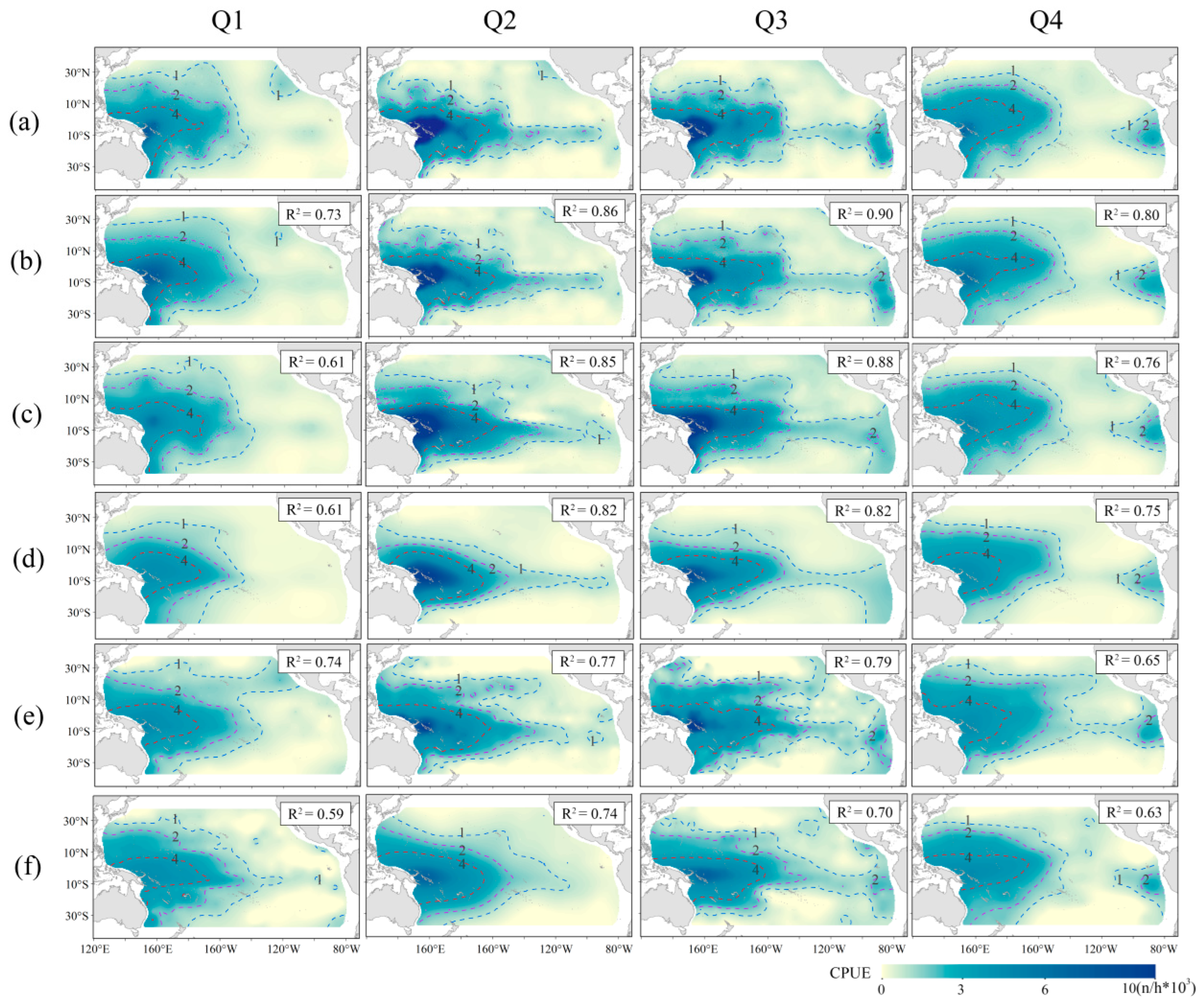
Table 4 compares the performance of the five models across the four quarters. Overall, GNNWR showed consistently strong performance across seasons. Although GWR slightly outperformed GNNWR on the test set in Q1, GNNWR achieved competitive performance across all four quarters, with particularly strong performance in the remaining seasons. The test-set performance of GNNWR was optimal in Q3, with an R2 of 0.902 and an RMSE of 0.977. These results indicate that GNNWR demonstrates generally robust performance across seasons while accounting for the nonlinear and spatially heterogeneous associations between nominal CPUE and environmental conditions.
Figure 2 depicts the spatial patterns of modeled nominal CPUE generated by the different models across the four quarters. Throughout the year, all models presented similar overall spatial trends. However, in Q3 and Q4, GAM and GWR significantly overestimated CPUE in the Northeast Pacific Ocean, displaying considerable fluctuations in the extent of high-value regions and indicating poor spatial stability. Meanwhile, the GNN model exhibited relatively smooth spatial patterns across all quarters, with limited representation of local spatial variation. GRF and GNNWR showed improved spatial agreement with the observed nominal CPUE patterns. Notably, GNNWR provided the most consistent spatial representation across all seasons, accurately reproducing both the distribution range and spatial gradients of high-CPUE regions, and exhibited the closest agreement with the observed patterns among all models.
To further assess model performance, we conducted a spatial visual analysis of the absolute errors for the five models across different quarters (Figure S2). The results demonstrated that the magnitude of spatial errors for GNNWR was consistently lower than that of GAM, GWR, GNN, and GRF in all quarters.
We also visualized the standardized residuals of the GNNWR model spatially for each quarter (Figure S3). The results indicated that the majority of grid-cell residuals fell within the relatively low interval of [−0.5, 0.5], with positive and negative residuals spatially dispersed and no apparent large-scale clusters of systematic overestimation or underestimation. Furthermore, Moran’s I tests were conducted for the standardized residuals (Table S4), and no statistically significant global spatial autocorrelation was detected in any quarter (all p > 0.05), suggesting that the major spatial structure was adequately accounted for by the GNNWR model.
Overall, the comparative results indicate that GNNWR outperforms the other models in both fitting accuracy and error metrics across seasons. Therefore, we selected GNNWR as the primary modeling approach for subsequent analyses in this study.

3.1.2. Independent-Year Validation of the GNNWR Model

To further evaluate the temporal transferability of the GNNWR model, an independent-year validation experiment was conducted using environmental conditions and observed nominal CPUE data from 2024. The trained seasonal models were applied to estimate yellowfin tuna CPUE distributions based on the environmental conditions of 2024, and the estimated results were compared with the corresponding observed nominal CPUE patterns.
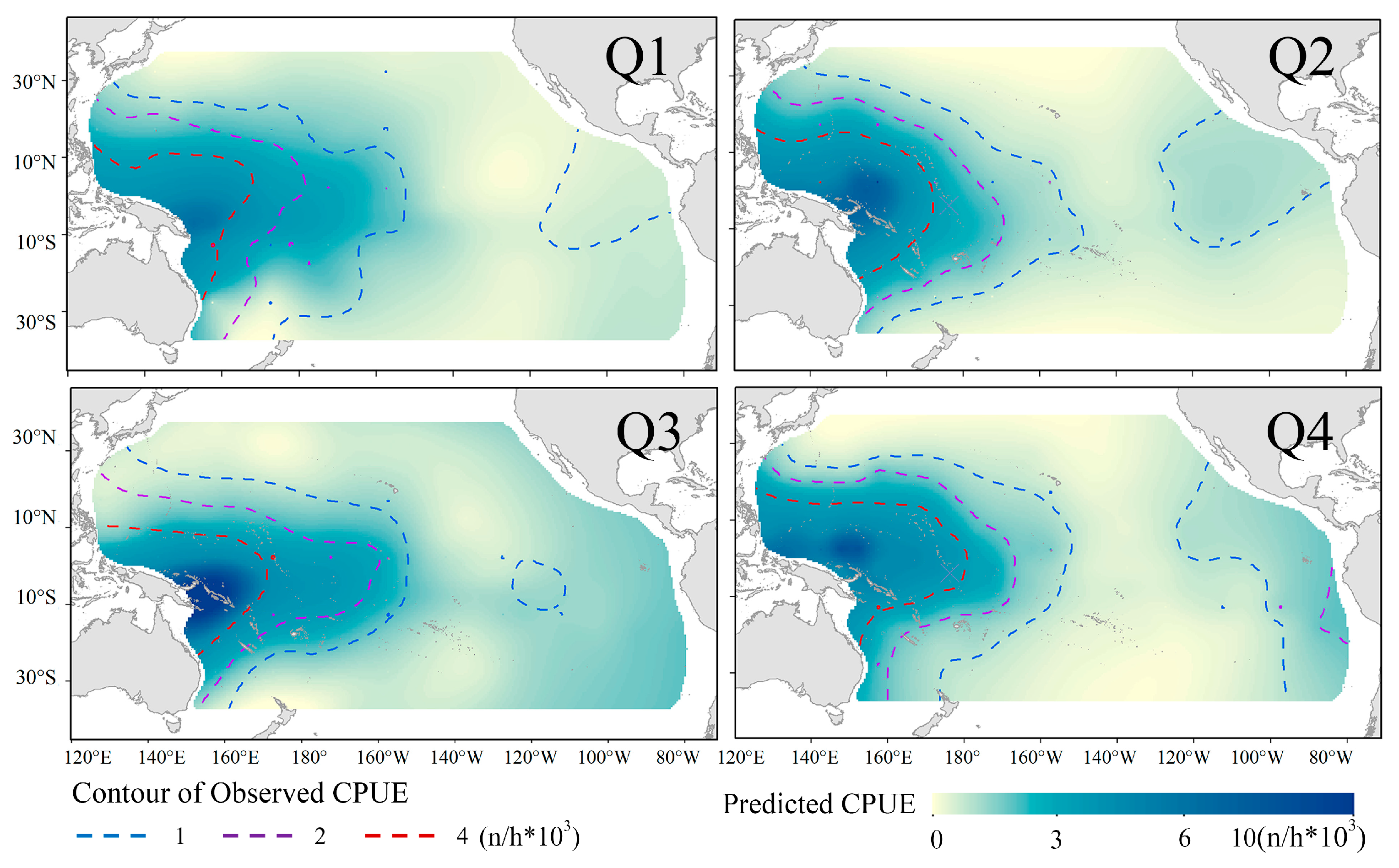
Table 5 summarizes the performance of the GNNWR model in the independent-year validation using the 2024 dataset. Across the four seasons, the model showed moderate agreement with the observed nominal CPUE, with R2 values ranging from 0.39 to 0.48. The highest performance was obtained in Q3 (R2 = 0.48, RMSE = 1.69, and MAE = 1.21). Although the model performance was lower than that obtained using the 20-year climatological dataset, the independent-year validation provides additional evidence regarding the temporal transferability of the model under environmental conditions from an independent year. The spatial comparison between observed and estimated CPUE distributions further indicated that the GNNWR model could reasonably reproduce the major spatial patterns of yellowfin tuna CPUE (Figure 3). Specifically, both the observed and estimated distributions consistently identified the central and western Pacific as regions with relatively high CPUE, whereas lower CPUE values were generally distributed in the eastern Pacific.
Overall, the independent-year validation suggests that the GNNWR model retains the ability to capture the large-scale spatial variability of yellowfin tuna nominal CPUE under different environmental conditions, supporting its applicability for characterizing spatially heterogeneous species–environment relationships.

3.2. Interpretation of the GNNWR Model Based on GeoShapley

3.2.1. The Ranking of the Importance of the Environmental and Spatial Factors

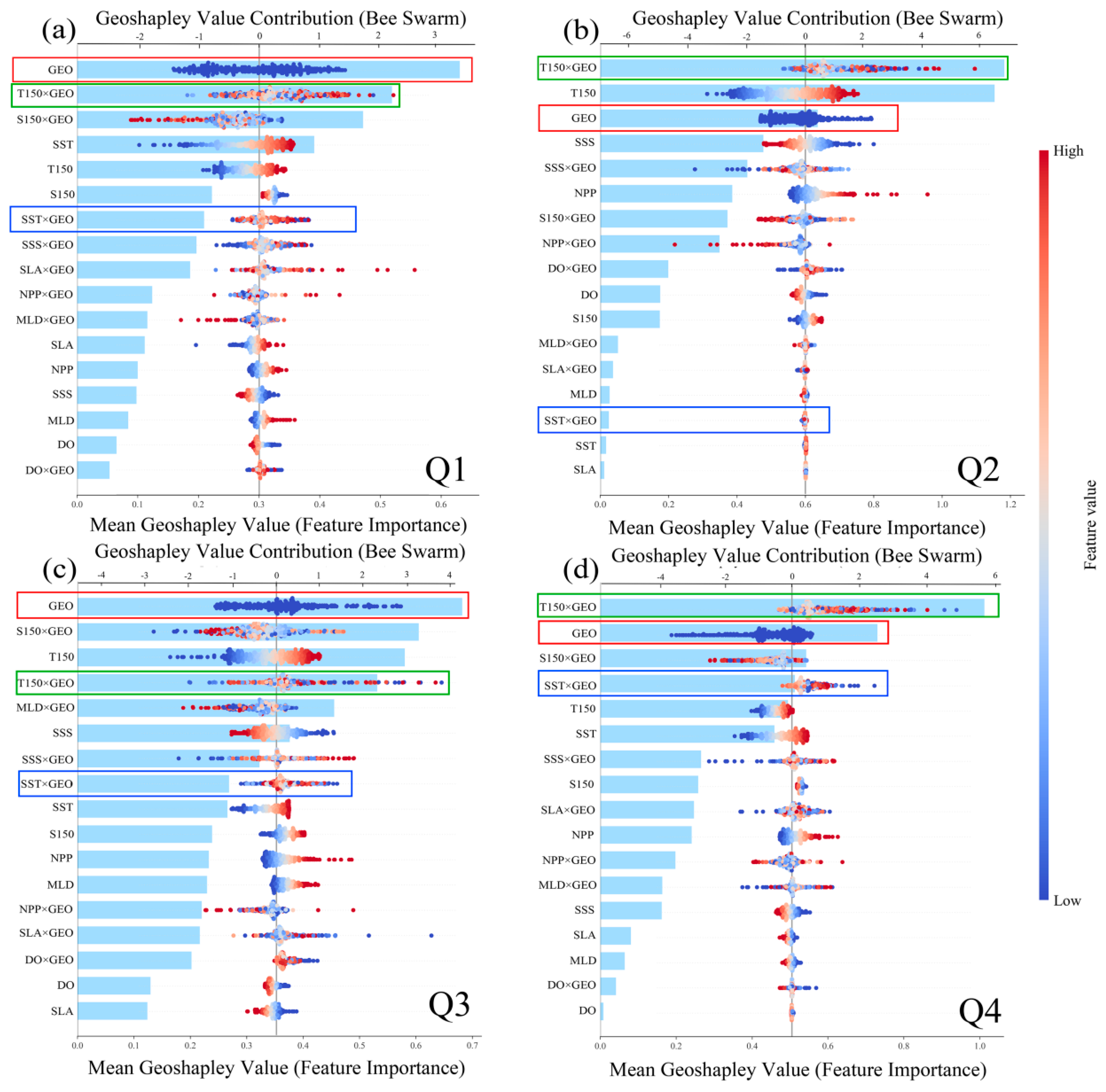
Figure 4 presents the global importance rankings of various environmental factors and their spatial interaction terms (×GEO) across the four quarters, illustrating the relative contributions of these factors to the GNNWR model output for Pacific yellowfin tuna nominal CPUE across seasons. Table S3 details the quantitative GeoShapley values for the top ten features.
The spatial effect (GEO), alongside surface and subsurface thermohaline variables and their spatial interactions, constituted the primary contributors of the model output. Notably, GEO consistently ranked in the top three across all seasons, acting as the dominant contributing factor in Q1 and Q3. Furthermore, the spatial interaction of subsurface temperature (T150 × GEO) contributed overwhelmingly in Q2 and Q4, yielding mean absolute GeoShapley values of 1.18 and 1.01, respectively (Table S3). While the main effect of T150 maintained persistently high importance year-round, SST and its interaction (SST × GEO) exhibited more pronounced seasonal fluctuations.
Beyond temperature, seawater salinity also showed high importance. Both the main effects of SSS and S150, as well as their interaction effects, made substantial contributions to the GNNWR model output. In contrast, NPP, MLD, SLA, and DO yielded relatively low GeoShapley values, indicating relatively lower contributions to modeled CPUE in the present analysis.

3.2.2. Response of Resource Abundance to Environmental Factors

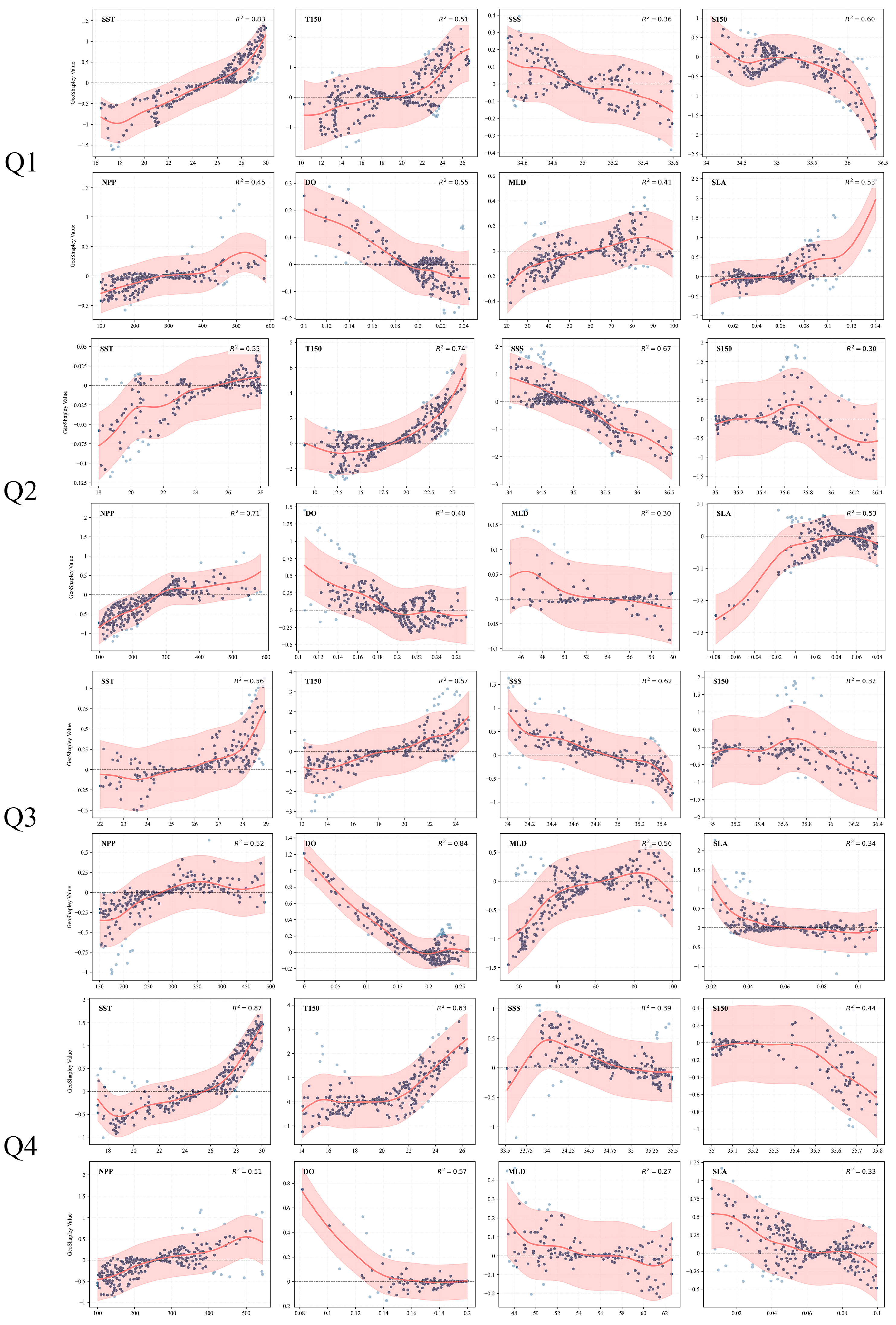
Figure 5 illustrates the marginal contribution curves of individual environmental factors to yellowfin tuna nominal CPUE, calculated while accounting for the contributions of the other factors. To characterize the nonlinear response patterns, generalized additive models (GAMs) were fitted to the discrete GeoShapley values. The GAM curves and their 95% confidence intervals provide a flexible representation of the nonlinear relationships and associated uncertainty without imposing a predefined functional form.
Our findings demonstrate pronounced nonlinear relationships between yellowfin tuna nominal CPUE and most environmental variables. Specifically, SST shows a transition from predominantly negative to positive model-derived contributions at approximately 25 °C, with the positive contribution increasing at higher values, particularly in Q1 and Q4. Similarly, T150 shows a model-derived turning point at approximately 19 °C, where its contribution shifts from negative to positive. Conversely to the temperature trends, the marginal effects of salinity (SSS and S150) decrease as their values increase, showing increasingly negative contributions when salinity exceeds 35 PSU. Furthermore, NPP shows increasingly positive model-derived contributions above approximately 300 mg/m2/day, while DO shows negative contributions when its value exceeds approximately 0.19 mol/m3. It should be noted that these patterns describe changes in the model-derived contributions of environmental variables, rather than direct causal effects or physiological thresholds.

3.2.3. Seasonal and Spatial Heterogeneity of Key Factors

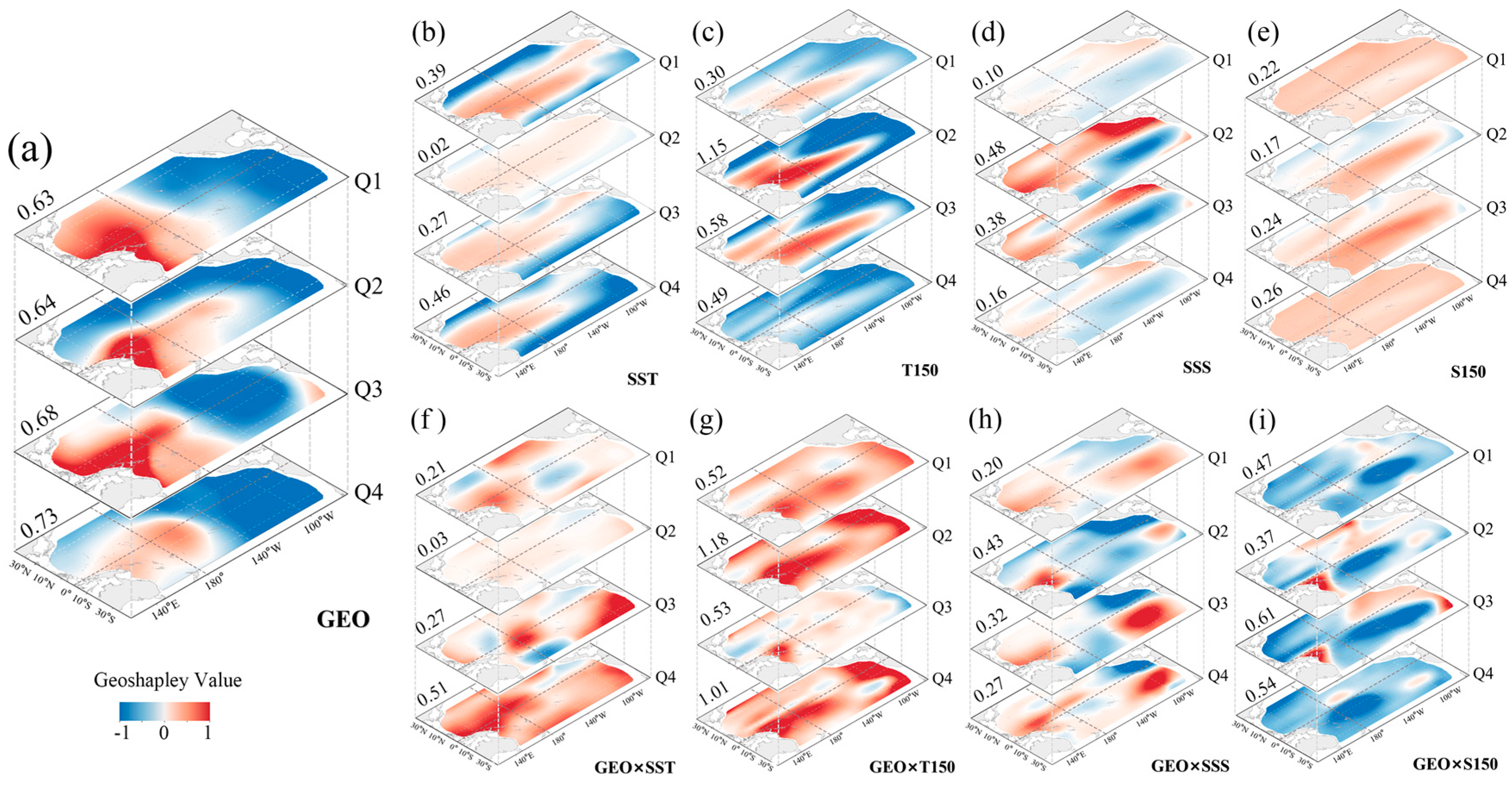
To further explore the seasonal and spatial variations of key factors, we mapped the localized GeoShapley values for the GEO, the main effects of four environmental factors (SST, T150, SSS, and S150), and their spatial interaction effects across the four quarters (Figure 6). The comparison reveals that different environmental factors exhibited significant spatiotemporal heterogeneity within the study area, with distinct differences in their contribution intensity and spatial extent across various oceanic regions and seasons.
The GEO generally showed a consistent “high in the west, low in the east” spatial distribution pattern across the four quarters, demonstrating pronounced spatial heterogeneity (Figure 6a). Although the exact spatial patterns fluctuated seasonally, positive GeoShapley contributions were persistently concentrated in the Western and Central Pacific Ocean. This indicates a relatively high positive contribution of the spatial component to modeled CPUE in these regions across seasons.
The main effect of SST primarily exhibited positive GeoShapley values along the equator in the Central Pacific, with a relatively weaker contribution in Q2 (Figure 6b). The incorporation of the spatial interaction term (Figure 6f) revealed that spatial location amplified the positive contribution of SST in the Central, Western, and parts of the Eastern Pacific. In contrast, the positive contributions of T150 was more concentrated, mainly locating in the Central and Western Pacific and extending eastward along the 20° S latitude (Figure 6c). Considering spatial interactions (Figure 6g), T150 × GEO displayed a widespread positive contribution, particularly significant in the Central and Western Pacific and the Eastern Pacific regions adjacent to the American continent.
The main effect of SSS exhibited a distinct north-south differentiation (Figure 6d), characterized by positive values in the North Pacific and negative values in the South. Its spatial interaction effect (SSS × GEO) showed concentrated high-value distributions in the Central, Western, and Eastern Pacific, indicating a pronounced spatial modulation effect (Figure 6h). While the main effect of S150 was largely positive (Figure 6e), combining it with the spatial effect (S150 × GEO) shifted it to a primarily negative contribution (Figure 6i), particularly in the Pacific south of the equator. Furthermore, its clustered areas of negative values exhibited a distinct westward shift across the seasons.

4. Discussion

4.1. Environmental Relationships of Key Factors with Pacific Yellowfin Tuna Nominal CPUE

Figure 4 shows that surface and subsurface temperature and salinity consistently ranked as the most important variables, highlighting the importance of the marine vertical thermohaline structure in characterizing spatial and seasonal variation in yellowfin tuna nominal CPUE.
As a typical warm-water species, the tuna’s metabolic rates, reproduction, and migratory behaviors are heavily regulated by seawater temperature [1]. Studies have shown that adult yellowfin tuna generally appear in waters with SST between 20 °C and 31 °C, while juveniles prefer warmer waters, primarily congregating in areas above 23 °C [24]. This aligns with the results displayed in the marginal effect plots (Figure 5), where SST was associated with positive contributions to modeled CPUE when exceeding 25 °C.
Furthermore, the mean absolute GeoShapley values for T150 and its spatial interaction (T150 × GEO) remained persistently high across all seasons, indicating their relatively high contributions to the GNNWR model output. Yellowfin tuna exhibit distinct diel vertical migration (DVM) behavior; at night, they are primarily distributed in the warm surface waters above the thermocline, whereas during the day, they frequently dive below the thermocline to forage, shuttling back and forth between the surface and deeper layers [25,26]. During typical foraging behavior, their daytime diving depths are generally concentrated between 50 and 300 m, and adult Pacific yellowfin tuna frequently operate and forage within the 150–250 m depth range [27,28]. Therefore, the 150 m water layer, often situated near the lower boundary of the thermocline, serves as a primary foraging habitat [29]. This depth range highly overlaps with the deployment depths of longline hooks. Such vertical overlap could potentially influence the likelihood of yellowfin tuna encountering fishing gear and, consequently, contribute to variations in observed nominal CPUE. Thus, the high importance of T150 may reflect its association with yellowfin tuna vertical habitat use and their availability to the fishery. Although the T150 depth range may overlap with the fishing depth of longline gear, this interpretation remains hypothetical because hook-depth and gear-configuration data were unavailable. Therefore, the importance of T150 should be interpreted as an environmental association with observed nominal CPUE rather than direct evidence of a fishing-depth overlap effect.
Beyond temperature, salinity also showed relatively high model contributions, particularly through its main and spatial interaction effects at 150 m. Salinity is related to environmental conditions that can affect physiological processes and prey distributions [30]. Our model revealed high importance for salinity and its spatial interactions, particularly at 150 m. Subsurface salinity stabilizes water stratification, creating deep-water environments favorable for prey aggregation and foraging. Marginal effect plots (Figure 5) demonstrated that SSS yielded positive contributions to CPUE below 34.9 but negative contributions above this threshold, while S150 exhibited a primarily inhibitory effect. This inhibition likely results from deepened stratification and restricted vertical mixing in high-salinity water masses. Furthermore, excessive salinity has been suggested to increase the metabolic costs associated with ionic balance in tuna, which may influence foraging activity and catchability [30,31]. Because S150 is more closely related to subsurface habitat conditions compared with SSS, it exhibited more prominent model importance. This also highlights the necessity of incorporating subsurface environmental variables into fishery resource modeling [19].

4.2. Spatial and Seasonal Variability in Environmental Associations

The spatial distribution of GEO exhibits a clear “high in the west and low in the east” pattern (Figure 6). This indicates that, across the study area, spatial variation in yellowfin tuna nominal CPUE is associated not only with the measured environmental variables but also with spatially structured factors that are not explicitly represented in the model. Firstly, the Central and Western Pacific has more suitable marine conditions for the survival of yellowfin tuna. As the world’s largest warm-water region, the Western Pacific “Warm Pool” provides a stable and optimal habitat for the thermophilic yellowfin tuna [32]. In contrast, the Eastern Pacific is influenced by the Peru Current and the equatorial upwelling system. These processes bring cold water to the surface, forming a low-temperature “Cold Tongue”, thereby suppressing the aggregation and distribution of yellowfin tuna [5]. In addition to these natural environmental impacts, human fishing activities have also reinforced the spatial clustering of CPUE. The longline tuna fishing industry has gradually formed relatively stable operational sea areas and empirical fishing grounds during the long-term production process, and the Central and Western Pacific, which contains important and historically established tuna fishing grounds, attracts a large number of fishing vessels to continuously concentrate their operations [33]. Under the combined effect of these multiple factors, the GEO variable in Figure 6a exhibited a prominent “high in the west, low in the east” distribution pattern. Additionally, the spatial effect represented by GEO may implicitly encapsulate latent factors that were not explicitly considered, which the GEO component of the GeoShapley framework captures effectively.
Beyond the geographic pattern, the contributions of sea surface and subsurface temperature to modeled CPUE also exhibit pronounced seasonal and spatial heterogeneity. The main effects of SST and T150 (Figure 6b,c) show spatial patterns broadly consistent with the distribution of the warm pool and cold tongue. This suggests that large-scale oceanographic structures may be reflected in the spatial variation of yellowfin tuna nominal CPUE. After introducing spatial interaction effects, the contributions of sea temperature to modeled CPUE show significant spatial heterogeneity, indicating that its effect is not uniform throughout the study area but is modulated by regional marine environments and ecological processes. Spatially, the Central and Western Pacific remain the core regions of high SST and T150 interaction effects, further highlighting the ecological significance of these regions. In the Eastern Pacific region near South America, the main effects of SST and T150 show negative constraints on CPUE, but their spatial interaction effects (SST × GEO, T150 × GEO) exhibit strong positive contributions. Although the surface water temperature in this region is lower, the upwelling brings a high-nutrient environment that can support high primary productivity [34], which may contribute to spatial variation in CPUE through changes in local oceanographic conditions and prey availability. This may partly explain the positive spatial interaction contributions observed in this region, particularly in Q2 and Q4.
In addition to spatial variations, the relative importance of sea surface and subsurface temperatures demonstrates a distinct seasonal variation. In Q2, both the main and interaction effects of SST reach their lowest levels (Figure 4 and Figure 6b,f), reducing its explanatory power. Meanwhile, T150 and T150 × GEO increase sharply, becoming the dominant environmental factors associated with CPUE. This shift may be related to seasonal changes in the western Pacific warm pool [35], during which spatial SST gradients may become weaker, while subsurface thermal conditions retain stronger spatial variation. As the warm pool contracts, SST gradients recover and the relative contribution of SST to modeled CPUE increases.
Salinity effects also exhibit clear spatial and seasonal variability. The main effect of SSS shows a strong north–south spatial contrast, while its interaction effect shows relatively high positive contributions near the Solomon Islands and in the southeastern Pacific. Near the Solomon Islands, complex topography–current interactions enhance mixing and local productivity, thereby promoting fish aggregation [36,37]. Conversely, in the southeastern Pacific, despite a negative main effect, the SSS × GEO becomes strongly positive during Q3 and Q4, coinciding spatially with the intensified Peru-Chile upwelling system [5]. Furthermore, the S150 × GEO exhibits significant negative clustering south of the equator, with its core area shifting westward seasonally. This spatial and seasonal variation may be associated with changes in the equatorial Cold Tongue and the periodic strengthening of the Southeast Trade Winds [38], which jointly enhance upwelling and contribute to seasonal changes in the subsurface hydrographic environment.

4.3. Performance Advantages and Applications of the GNNWR-GeoShapley Framework

The GNNWR model integrates neural networks with geographically weighted regression, substantially expanding the capacity of spatial regression methods to capture complex, nonlinear relationships [22]. In this study, GNNWR demonstrated generally strong performance across the four quarters. Although GRF and GNN also demonstrated strong capability in capturing nonlinear relationships, GNNWR showed good overall performance and spatial consistency, particularly in representing spatial gradients and variations of CPUE (Figure 2), while maintaining relatively low residual errors across the study area (Figure S2). Moreover, the visualization of GeoShapley results indicated that GNNWR provided a more effective characterization of spatial heterogeneity (Figure 6), supporting its ability to characterize spatially varying environmental associations.
Although marine ecosystems are characterized by dynamic processes, fluid boundaries, and strong oceanographic connectivity, these features can still generate spatially heterogeneous CPUE–environment relationships across different regions. In this context, the distance-based weighting in GNNWR is not intended to represent fixed ecological boundaries, but rather to characterize location-dependent variations in the relationships between nominal CPUE and environmental conditions. Combined with the nonlinear learning capability of neural networks, GNNWR therefore provides a spatially explicit approach for investigating spatially heterogeneous CPUE–environment associations in pelagic ecosystems. However, GNNWR does not explicitly represent all dynamic processes operating within oceanic ecosystems; rather, it is intended to characterize the geographic variation in the statistical relationships between nominal CPUE and environmental conditions.
To further assess the applicability of the CPUE–environment relationships identified by GNNWR under independent annual conditions, an additional validation experiment was conducted using environmental data from 2024. Although the model performance was lower than that obtained using the 20-year averaged dataset, it reasonably reproduced the major spatial patterns of yellowfin tuna nominal CPUE. Rather than evaluating the model’s forecasting capability, this experiment was designed to examine the robustness of the identified relationships under an independent annual environmental state.
More importantly, the integration of GeoShapley substantially improved the interpretability of the GNNWR framework. Unlike traditional global importance measures, GeoShapley enables the quantification of spatially varying contributions from environmental factors and their interactions, providing a more detailed understanding of environment-related CPUE distribution patterns. The results revealed that the contributions of key environmental variables varied considerably across seasons and geographic regions, highlighting the importance of considering spatial heterogeneity when interpreting CPUE–environment associations.
Compared with previous machine learning approaches, the GNNWR–GeoShapley framework provides a spatially explicit framework for characterizing nonlinear and spatially heterogeneous CPUE–environment relationships. This framework does not aim to replace conventional stock assessment approaches, but offers a complementary approach for investigating the complex associations between environmental conditions and nominal CPUE. Given the complex environmental gradients and extensive spatial variability of pelagic ecosystems, the proposed framework can help characterize how these associations vary across different seasons and geographic regions, providing insights for ecosystem-based fisheries research.

4.4. Considerations for Interpreting CPUE—Environment Relationships

In this study, nominal CPUE was used because complete operational information required for CPUE standardization, including hook depth, bait type, vessel-specific fishing practices, and targeting behavior, was not consistently available. It is important to recognize that CPUE represents the outcome of both the availability of yellowfin tuna and the probability of their capture. Consequently, spatial or seasonal differences in fishing practices may be reflected in CPUE variation alongside changes associated with environmental conditions. This is particularly relevant in pelagic fisheries, where fishing depth and targeting strategies can vary according to the expected distribution of different tuna species. For example, changes in hook depth may alter the vertical range of the fishing gear and hence the probability of encountering yellowfin tuna, even under similar environmental conditions.
Such variation in catchability does not necessarily invalidate the observed CPUE–environment relationships, but it may affect their magnitude and spatial expression. When fishing practices and environmental conditions vary concurrently, part of the apparent environmental association may reflect differences in fishing operations rather than the ecological response of yellowfin tuna alone. Conversely, if fishing practices are relatively consistent within particular areas or seasons, the observed spatial patterns may still contain meaningful information on the environmental conditions associated with yellowfin tuna occurrence. Therefore, the environmental relationships identified here are best viewed as relationships with observed CPUE that integrate ecological and fishery-related processes. Incorporating more comprehensive operational information and standardized CPUE in future studies would help further distinguish these components and provide a more refined understanding of the underlying species–environment relationships.

5. Conclusions

This study developed an interpretable spatial modeling framework by integrating Geographically Neural Network Weighted Regression (GNNWR) with GeoShapley analysis to investigate the complex relationships between environmental conditions and Pacific yellowfin tuna nominal CPUE. By combining nonlinear learning capability with spatially explicit modeling, the proposed framework provides a comprehensive approach for characterizing nonlinear and spatially heterogeneous CPUE–environment associations across a large-scale marine ecosystem.
Our results identified vertical ocean thermohaline structure as one of the most important environmental factors associated with yellowfin tuna nominal CPUE patterns. Subsurface environments, particularly at 150 m, showed consistent contributions to model output across seasons, highlighting the importance of vertical habitat structure in explaining the distribution patterns of pelagic top predators. Importantly, the magnitude and spatial extent of these environmental contributions varied markedly across seasons. Furthermore, the spatial effect (GEO) and its interactions with local environmental variables were identified as important contributors to model output, indicating that spatial context plays an important role in explaining variations in yellowfin tuna nominal CPUE patterns beyond environmental conditions alone. The GeoShapley framework further enhanced model interpretability by quantitatively characterizing the spatially varying contributions of environmental variables and highlighting the value of spatially explicit modeling for understanding species–environment relationships in fisheries science.
This study also has several limitations. The current analysis was based on quarterly averaged CPUE and environmental conditions, which effectively captured broad seasonal spatial patterns but may not fully represent short-term ecological variability. Because the model was developed using 20-year averaged environmental conditions and CPUE, its application to annual environmental states may be affected by differences in temporal scales and interannual variability. In addition, limited operational fishing information restricted further CPUE standardization and the separation of ecological signals from fishing-related effects. Although GNNWR accounts for spatially varying relationships, its performance relative to other advanced spatially heterogeneous modelling frameworks remains to be further evaluated. Future studies incorporating higher-resolution temporal observations, detailed fishing operation variables, and multi-depth environmental profiles may further improve the characterization of yellowfin tuna nominal CPUE variability. Moreover, the relationships identified by GeoShapley represent model-based associations rather than direct causal effects and should be further evaluated using independent ecological observations.
Overall, the GNNWR-GeoShapley framework provides a powerful and interpretable approach for revealing nonlinear and spatially heterogeneous species–environment relationships. This study demonstrates the potential of spatially explicit artificial intelligence methods for improving ecological interpretation and sustainable management of Pacific pelagic resources.

Supplementary Materials

The following supporting information can be downloaded at: https://www.mdpi.com/article/10.3390/fishes11090539/s1, Text S1: Selection of Environmental Variables; Text S2: Implementation of five-fold cross-validation; Text S3: Construction of the GAM Model; Text S4: Construction of the GWR Model; Text S5: Construction of the GNN Model; Text S6: Construction of the GRF Model; Text S7: Introduction to the GeoShapley Method; Figure S1: Spearman correlation analysis between environmental factors and CPUE across four quarters; Figure S2: Absolute Errors of Different Models.(a) GAM, (b) GWR, (c) GNN, (d) GRF, (e) GNNWR; Figure S3: Spatial distribution of standardized residuals for GNNWR; Table S1: R2 from five-fold cross-validation for GAM, GWR, GNN, GRF and GNNWR; Table S2: RMSE from five-fold cross-validation for GAM, GWR, GNN, GRF and GNNWR; Table S3: Statistical summary of GeoShapley values for environmental factors and geographic interactions across four quarters; Table S4: Global Moran’s I test results for standardized residuals of the GNNWR model [1,18,19,31,32,39,40,41,42].

Author Contributions

Conceptualization, M.L. and X.Y.; methodology, M.L.; software, Z.H.; validation, M.L., Z.H. and X.Y.; formal analysis, X.Y.; investigation, M.L.; resources, J.Z.; data curation, Z.H.; writing—original draft preparation, M.L.; writing—review and editing, M.L.; visualization, M.L.; supervision, X.Y.; project administration, X.Y.; funding acquisition, J.Z. All authors have read and agreed to the published version of the manuscript.

Funding

This work was supported by National Key R&D Program of China under the project “Scientific and Technological Innovation in Marine Agriculture and Freshwater Fisheries” (2024YFD2400603) and the Dynamic Monitoring and Assessment Project for Globally Important Fish Resources (2025) funded by the Ministry of Agriculture and Rural Affairs of the People’s Republic of China (D-8025-25-5002).

Institutional Review Board Statement

Not applicable.

Informed Consent Statement

Not applicable.

Data Availability Statement

The data that support the findings of this study are available from the corresponding author upon reasonable request.

Acknowledgments

This project was funded in part by the National Key Research and Development Program of China. We thank all our colleagues from the Research Laboratory for their work during data collection.

Conflicts of Interest

The authors declare no conflicts of interest.

References

  1. Pecoraro, C.; Zudaire, I.; Bodin, N.; Murua, H.; Taconet, P.; Díaz-Jaimes, P.; Cariani, A.; Tinti, F.; Chassot, E. Putting all the pieces together: Integrating current knowledge of the biology, ecology, fisheries status, stock structure and management of yellowfin tuna (Thunnus albacares). Rev. Fish Biol. Fish. 2016, 27, 811–841. [Google Scholar] [CrossRef] [Scilit]
  2. Báez, J.C.; Czerwinski, I.A.; Ramos, M.L.; Bellido, J.M.; Coll, M. New Fishing Strategies to Face Climate Change Effects on the Spanish Tropical Tuna Fisheries off Indian Ocean. Fish. Oceanogr. 2025, 34, 17–26. [Google Scholar] [CrossRef] [Scilit]
  3. Western and Central Pacific Fisheries Commission (WCPFC). WCPFC Tuna Fishery Yearbook 2025 (with Data Available Through 2024); Pacific Community (SPC) & WCPFC: Noumea, New Caledonia, 2025; Available online: https://www.wcpfc.int (accessed on 1 May 2026).
  4. Brill, R.W.; Block, B.A.; Boggs, C.H.; Bigelow, K.A.; Freund, E.V.; Marcinek, D.J. Horizontal movements and depth distribution of large adult yellowfin tuna (Thunnus albacares) near the Hawaiian Islands, recorded using ultrasonic telemetry: Implications for the physiological ecology of pelagic fishes. Mar. Biol. 1999, 133, 395–408. [Google Scholar] [CrossRef] [Scilit]
  5. Hua, Z.; Yang, X.; Li, M.; Feng, S.; Zhu, J. Spatial Heterogeneity-Based Explainable Machine Learning Methods—Modeling the Relationship Between Yellowfin Tuna Fishery Resources and the Environment in the Pacific Ocean. Fishes 2025, 10, 417. [Google Scholar] [CrossRef] [Scilit]
  6. Langley, A.; Harley, S.; Hoyle, S.; Davies, N.; Hampton, J.; Kleiber, P. Stock Assessment of Yellowfin Tuna in the Western and Central Pacific Ocean, in WCPFC SC5 SA WP-3, Port Vila, Vanuatu; Western and Central Pacific Fisheries Commission (WCPFC): Port Vila, Vanuatu, 2009; pp. 10–21. [Google Scholar]
  7. Setiawati, M.D.; Sambah, A.B.; Miura, F.; Tanaka, T.; As-Syakur, A.R. Characterization of bigeye tuna habitat in the Southern Waters off Java–Bali using remote sensing data. Adv. Space Res. 2015, 55, 732–746. [Google Scholar] [CrossRef] [Scilit]
  8. Schick, R.; Lutcavage, M.E. Inclusion of prey data improves prediction of bluefin tuna (Thunnus thynnus) distribution. Fish. Oceanogr. 2009, 18, 77–81. [Google Scholar] [CrossRef] [Scilit]
  9. Jiang, S.; Yang, X.; Zhu, J. Analysis of spatial and temporal heterogeneity of the relationship between skipjack tuna fishery and marine environment in the Western and Central Pacific Ocean. J. Fish. China 2022, 29, 744–754, (In Chinese with English abstract). [Google Scholar] [CrossRef]
  10. Zheng, H.; Yang, X.; Zhu, J. Environmental impact mechanism of skipjack tuna fishery in Western and Central Pacific Ocean based on Multi-scale Geographical Weighted Regression Model (MGWR). South China Fish. Sci. 2023, 19, 1–10, (In Chinese with English abstract). [Google Scholar] [CrossRef]
  11. Song, B.; Liu, J.; Zhang, T.; Chen, Q. A Hybrid Deep Learning Model for Predicting Tuna Distribution Around Drifting Fish Aggregating Devices. Sustainability 2026, 18, 2406. [Google Scholar] [CrossRef] [Scilit]
  12. Yang, L.; Zhou, W.; Zhang, C.; Tang, F. A comparative machine learning study identifies light gradient boosting machine (lightgbm) as the optimal model for unveiling the environmental drivers of yellowfin tuna (Thunnus albacares) distribution using shapley additive explanations (shap) analysis. Biology 2025, 14, 1567. [Google Scholar] [CrossRef] [Scilit]
  13. Ienaga, N.; Higuchi, K.; Takashi, T.; Gen, K.; Tsuda, K.; Terayama, K. Vision-based egg quality prediction in Pacific bluefin tuna (Thunnus orientalis) by deep neural network. Sci. Rep. 2021, 11, 6. [Google Scholar] [CrossRef] [Scilit]
  14. Wang, Z.; Wang, Y.; Wu, S.; Du, Z. House Price Valuation Model Based on Geographically Neural Network Weighted Regression: The Case Study of Shenzhen, China. ISPRS Int. J. Geo-Inf. 2022, 11, 450. [Google Scholar] [CrossRef] [Scilit]
  15. Du, Z.; Wang, Z.; Wu, S.; Zhang, F.; Liu, R. Geographically neural network weighted regression for the accurate estimation of spatial non-stationarity. Int. J. Geogr. Inf. Sci. 2020, 34, 1353–1377. [Google Scholar] [CrossRef] [Scilit]
  16. Qi, J.; Du, Z.; Wu, S.; Chen, Y.; Wang, Y. A spatiotemporally weighted intelligent method for exploring fine-scale distributions of surface dissolved silicate in coastal seas. Sci. Total Environ. 2023, 886, 163981. [Google Scholar] [CrossRef] [Scilit]
  17. Zhang, Z.; Wu, S.; Zhang, B.; Du, Z.; Xia, Q. The Distribution of Surface Heat Flow on the Tibetan Plateau Revealed by Data-Driven Methods. J. Geophys. Res. Solid Earth 2024, 129, e2023JB028491. [Google Scholar] [CrossRef] [Scilit]
  18. Li, Z. GeoShapley: A Game Theory Approach to Measuring Spatial Effects in Machine Learning Models. Ann. Am. Assoc. Geogr. 2024, 114, 1365–1385. [Google Scholar] [CrossRef] [Scilit]
  19. Li, M.; Yang, X.; Wang, Y.; Wang, Y.; Zhu, J. The Use of the GWPCA-MGWR Model for Studying Spatial Relationships between Environmental Variables and Longline Catches of Yellowfin Tunas. J. Mar. Sci. Eng. 2024, 12, 1002. [Google Scholar] [CrossRef] [Scilit]
  20. Hilborn, R.; Walters, C.J. Quantitative Fisheries Stock Assessment: Choice, Dynamics and Uncertainty; Springer Science & Business Media: Berlin/Heidelberg, Germany, 2013. [Google Scholar]
  21. Beverton, R.J.H.; Holt, S.J. On the Dynamics of Exploited Fish Populations; Fishery Investigations Series II. Vol. Fishery Investigations Series II, No. 19; Her Majesty’s Stationery Office: London, UK, 1957. [Google Scholar]
  22. Chen, Y.; Wu, S.; Wang, Y.; Zhang, F.; Liu, R.; Du, Z. Satellite-Based Mapping of High-Resolution Ground-Level PM2.5 with VIIRS IP AOD in China through Spatially Neural Network Weighted Regression. Remote Sens. 2021, 13, 1979. [Google Scholar] [CrossRef] [Scilit]
  23. Guang, X.; Xiang, L.; He, Y.; Zhang, N.; Zheng, J.; Qin, Y.; Kong, D.; Wang, H.; Lin, L.; Zhu, B. Development and validation of a Geospatial eXplainable Artificial Intelligence (GeoXAI) framework for mapping mosquito density in metropolitans. Appl. Geogr. 2025, 181, 103685. [Google Scholar] [CrossRef] [Scilit]
  24. Reglero, P.; Tittensor, D.; Álvarez-Berastegui, D.; Aparicio-González, A.; Worm, B. Worldwide distributions of tuna larvae: Revisiting hypotheses on environmental requirements for spawning habitats. Mar. Ecol. Prog. Ser. 2014, 501, 207–224. [Google Scholar] [CrossRef] [Scilit]
  25. Schaefer, K.M.; Fuller, D.W.; Aldana, G. Movements, behavior, and habitat utilization of yellowfin tuna (Thunnus albacares) in waters surrounding the Revillagigedo Islands Archipelago Biosphere Reserve, Mexico. Fish. Oceanogr. 2013, 23, 65–82. [Google Scholar] [CrossRef] [Scilit]
  26. Hoolihan, J.P.; Wells, R.J.D.; Luo, J.; Falterman, B.; Prince, E.D.; Rooker, J.R. Vertical and horizontal movements of yellowfin tuna in the Gulf of Mexico. Mar. Coast. Fish. 2014, 6, 211–222. [Google Scholar] [CrossRef] [Scilit]
  27. Schaefer, K.M.; Fuller, D.W.; Block, B.A. Vertical Movements and Habitat Utilization of Skipjack (Katsuwonus pelamis), Yellowfin (Thunnus albacares), and Bigeye (Thunnus obesus) Tunas in the Equatorial Eastern Pacific Ocean, Ascertained Through Archival Tag Data. Reviews: Methods and Technologies in Fish Biology and Fisheries; Springer: Berlin/Heidelberg, Germany, 2009; pp. 121–144. [Google Scholar] [CrossRef] [Scilit]
  28. Schaefer, K.M.; Fuller, D.W.; Block, B.A. Movements, behavior, and habitat utilization of yellowfin tuna (Thunnus albacares) in the northeastern Pacific Ocean, ascertained through archival tag data. Mar. Biol. 2007, 152, 503–525. [Google Scholar] [CrossRef] [Scilit]
  29. Houssard, P.; Lorrain, A.; Tremblay-Boyer, L.; Allain, V.; Graham, B.S.; Menkes, C.E.; Pethybridge, H.; Couturier, L.I.; Point, D.; Leroy, B.; et al. Trophic position increases with thermocline depth in yellowfin and bigeye tuna across the Western and Central Pacific Ocean. Prog. Oceanogr. 2017, 154, 49–63. [Google Scholar] [CrossRef] [Scilit]
  30. Maury, O.; Gascuel, D.; Marsac, F.; Fonteneau, A.; De Rosa, A.-L. Hierarchical interpretation of nonlinear relationships linking yellowfin tuna (Thunnus albacares) distribution to the environment in the Atlantic Ocean. Can. J. Fish. Aquat. Sci. 2001, 58, 458–469. [Google Scholar] [CrossRef]
  31. Song, L.M.; Zhang, Y.; Xu, L.X.; Jiang, W.X.; Wang, J.Q. Environmental preferences of longlining for yellowfin tuna (Thunnus albacares) in the tropical high seas of the Indian Ocean. Fish. Oceanogr. 2008, 17, 239–253. [Google Scholar] [CrossRef] [Scilit]
  32. Lan, K.-W.; Shimada, T.; Lee, M.-A.; Su, N.-J.; Chang, Y. Using Remote-Sensing Environmental and Fishery Data to Map Potential Yellowfin Tuna Habitats in the Tropical Pacific Ocean. Remote Sens. 2017, 9, 444. [Google Scholar] [CrossRef] [Scilit]
  33. Miller, M.M.; Bush, S.R.; van Zwieten, P.A. Sub-regionalisation of fisheries governance: The case of the Western and Central Pacific Ocean tuna fisheries. Marit. Stud. 2014, 13, 17. [Google Scholar] [CrossRef] [Scilit]
  34. Hauschildt, J.; Thomsen, S.; Echevin, V.; Oschlies, A.; José, Y.S.; Krahmann, G.; Bristow, L.A.; Lavik, G. The fate of upwelled nitrate off Peru shaped by submesoscale filaments and fronts. Biogeosciences 2021, 18, 3605–3629. [Google Scholar] [CrossRef] [Scilit]
  35. Yin, Z.; Dong, Q.; Kong, F.; Cao, D.; Long, S. Seasonal and interannual variability of the Indo-Pacific Warm Pool and its associated climate factors based on remote sensing. Remote Sens. 2020, 12, 1062. [Google Scholar] [CrossRef] [Scilit]
  36. Srinivasan, K.; Renault, L.; McWilliams, J.C. Varieties of Submesoscale Dynamics in the South-West Pacific. In Ocean Sciences Meeting; American Geophysical Union: Washington, DC, USA, 2016. [Google Scholar]
  37. Sun, Y.; Wang, Y.-C.; Hsu, L.-H.; Meng, P.-J.; Hsieh, H.-Y. Upwelling as a nursery for fish larvae: Summer observations from the Taiwan Bank. Reg. Stud. Mar. Sci. 2026, 95, 104831. [Google Scholar] [CrossRef] [Scilit]
  38. Moum, J.N.; Perlin, A.; Nash, J.D.; McPhaden, M.J. Seasonal sea surface cooling in the equatorial Pacific cold tongue controlled by ocean mixing. Nature 2013, 500, 64–67. [Google Scholar] [CrossRef] [Scilit]
  39. Deary, A.L.; Moret-Ferguson, S.; Engels, M.; Zettler, E.; Jaroslow, G.; Sancho, G. Influence of Central Pacific Oceanographic Conditions on the Potential Vertical Habitat of Four Tropical Tuna Species. Pac. Sci. 2015, 69, 461–475. [Google Scholar] [CrossRef] [Scilit]
  40. Leung, S.; Thompson, L.; McPhaden, M.J.; Mislan, K.A.S. ENSO drives near-surface oxygen and vertical habitat variability in the tropical Pacific. Environ. Res. Lett. 2019, 14, 064020. [Google Scholar] [CrossRef] [Scilit]
  41. Zagaglia, C.R.; Lorenzzetti, J.A.; Stech, J.L. Remote sensing data and longline catches of yellowfin tuna (Thunnus albacares) in the equatorial Atlantic. Remote Sens. Environ. 2004, 93, 267–281. [Google Scholar] [CrossRef] [Scilit]
  42. Ziegel, E.R. Geographically Weighted Regression. Technometrics 2006, 48, 149. [Google Scholar] [CrossRef] [Scilit]
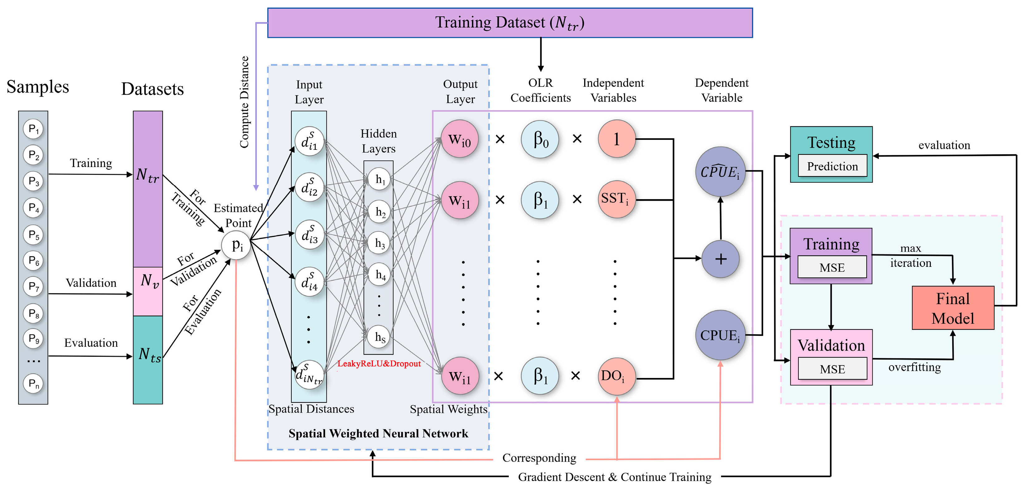
Figure 1. The CPUE estimation process of the GNNWR model.
Fishes 11 00539 g001
Figure 2. Comparison of Mode Performance. (a) True nominal CPUE, (b) GNNWR, (c) GRF, (d) GNN, (e) GWR, (f) GAM. The blue, purple, and red dashed lines represent CPUE isolines of 1, 2, and 4, respectively, with units of n/h × 103 (numbers per 1000 hooks).
Fishes 11 00539 g002
Figure 3. Spatial comparison between observed and predicted nominal CPUE distributions in 2024. Contour lines represent the spatial distribution of observed CPUE values, while the color-gradient background indicates the spatial patterns of predicted CPUE, with color intensity reflecting the relative magnitude of predicted values.
Fishes 11 00539 g003
Figure 4. Quarterly GeoShapley analysis of environmental factors for Pacific yellowfin tuna nominal CPUE. (a), (b), (c) and (d) represent the results for Q1–Q4, respectively. The bar chart presents the mean absolute GeoShapley values, illustrating the average impact of each feature on the model output. The beeswarm plot demonstrates the impact of individual sample points on the model output. The position of the points along the x-axis is determined by the corresponding GeoShapley values; a greater distance from the centerline indicates a stronger impact on the model output, with positive and negative GeoShapley values indicating positive and negative contributions to modeled CPUE, respectively. Each point’s color is mapped to the raw value of the corresponding feature, with a blue-to-red spectrum indicating low-to-high measurements. “GEO” denotes the location factor, for which the color assignment does not represent a numerical magnitude. In addition, three relatively special factors are highlighted with red, blue, and green boxes in the figure to facilitate comparative analysis.
Fishes 11 00539 g004
Figure 5. Seasonal nonlinear marginal contributions of environmental factors to yellowfin tuna nominal CPUE derived from GeoShapley analysis. Blue dots represent individual sample observations, while the red solid line indicates the GAM-fitted curve. The gray dashed horizontal line represents a GeoShapley value of zero, indicating no marginal contribution of the corresponding environmental factor to the model output. The pink shaded area represents the 95% confidence interval. The upper right corner of each subplot displays the coefficient of determination (R2) for the corresponding GAM fit. The x-axis represents the value range of the environmental factor, and the y-axis denotes the marginal contribution (GeoShapley value) of that factor to the model output.
Fishes 11 00539 g005
Figure 6. Seasonal and spatial distribution patterns of GeoShapley values for environmental factors and their spatial interactions. Pictures illustrate the localized contributions of: (a) The spatial effect (GEO); (be) main environmental factors (SST, T150, SSS, and S150); and (fi) their respective spatial interaction effects (×GEO). Red and blue areas indicate positive and negative contributions to model output, respectively. The mean absolute GeoShapley value is annotated in the upper left corner of each subplot.
Fishes 11 00539 g006
Table 1. Basic information of environmental variables.
VariablesUnitSpatial ResolutionData Source
SST, T50, T100,
T150, T200
SSS, S50, S100,
S150, S200
°C1° × 1°https://www.argo.org.cn/
(accessed on 15 March 2025)
PSU1° × 1°
U5, U55, U105,
V5, V55, V105
m/s0.333° × 1°https://ftp.cpc.ncep.noaa.gov/
(accessed on 15 March 2025)
MLD
CHL
NPP
m
mg/m3
mg/m2/day
0.167° × 0.167°https://orca.science.oregonstate.edu/
(accessed on 15 March 2025)
SLAm0.25° × 0.25°https://cds.climate.copernicus.eu/
(accessed on 15 March 2025)
DOmol/m31° × 1°https://aims2.llnl.gov/search/cmip6/
(accessed on 15 March 2025)
Note: SST, T50, T100, T150, and T200 represent water temperatures at different depths; SSS, S50, S100, S150, and S200 represent salinities at different depths; U5, U55, U105, V5, V55, and V105 denote ocean current velocities at various depths, where U represents the zonal (east-west) velocity and V represents the meridional (north-south) velocity; MLD stands for mixed layer depth; CHL is chlorophyll concentration; NPP is net primary productivity; SLA is sea level anomaly; and DO represents dissolved oxygen concentration at the shallowest local minimum in the vertical dissolved oxygen profile.
Table 2. VIF values of key environmental variables for the four seasons.
VariablesVIF Values ≤ 7.5 Correlation   Coefficient ≥ 0.7
Q1Q2Q3Q4
SST6.755.775.215.27T50, T100
T1506.813.776.147.06T200, S100
SSS3.083.003.454.88S50, S100, V5
S1506.864.837.177.12S100, S200, V5
MLD3.641.653.711.74
SLA1.271.361.351.16
NPP1.812.122.561.60CHl
DO2.602.371.442.55
Note: The table presents the VIF values of the selected environmental variables and the factors strongly correlated with them in the Spearman analysis across four quarters. Detailed correlation results are shown in Figure S1.
Table 3. Settings of architectures and hyperparameters for the GNNWR model.
Hidden Layer 1Hidden Layer 2Hidden Layer 3Output LayerLearning RateMax EpochsBatch SizeDropout
128643290.0012000160.5
Table 4. Performance comparison of GAM, GWR, GNN, GRF and GNNWR based on five-fold cross-validation.
R2RMSE
SeasonModelTrainValidTestTrainValidTest
Q1GAM0.693 ± 0.0080.660 ± 0.0530.5881.091 ± 0.0201.137 ± 0.1031.425
GWR0.719 ± 0.0090.674 ± 0.0200.7441.044 ± 0.0261.108 ± 0.0621.123
GNN0.715 ± 0.0290.651 ± 0.0450.6141.050 ± 0.0461.154 ± 0.0941.380
GRF0.808 ± 0.0070.686 ± 0.0400.6130.864 ± 0.0021.093 ± 0.0821.381
GNNWR 0.799 ± 0.025 0.714 ± 0.0560.7330.881 ± 0.0531.042 ± 0.1311.148
Q2GAM0.788 ± 0.0180.631 ± 0.0630.7371.256 ± 0.1211.616 ± 0.3311.575
GWR0.759 ± 0.0130.697 ± 0.0310.7701.339 ± 0.1011.475 ± 0.3311.279
GNN0.837 ± 0.0180.808 ± 0.0360.8221.099 ± 0.0931.182 ± 0.3441.125
GRF0.841 ± 0.0100.774 ± 0.0620.8451.086 ± 0.0891.238 ± 0.3891.020
GNNWR0.842 ± 0.0330.788 ± 0.0750.8641.132 ± 0.1421.236 ± 0.3100.983
Q3GAM0.707 ± 0.0330.582 ± 0.1070.6951.266 ± 0.0531.467 ± 0.2171.723
GWR0.738 ± 0.0260.645 ± 0.0540.7861.204 ± 0.0801.329 ± 0.1341.442
GNN0.797 ± 0.0300.709 ± 0.0880.8201.051 ± 0.0611.061 ± 0.2601.323
GRF0.877 ± 0.0080.716 ± 0.0600.8760.821 ± 0.0281.225 ± 0.2441.007
GNNWR0.868 ± 0.0090.767 ± 0.0820.9020.850 ± 0.0411.088 ± 0.2370.977
Q4GAM0.772 ± 0.0140.636 ± 0.0790.6340.988 ± 0.0391.246 ± 0.2401.284
GWR0.755 ± 0.0080.689 ± 0.0620.6511.024 ± 0.0321.130 ± 0.1941.254
GNN0.728 ± 0.0620.658 ± 0.1070.7511.074 ± 0.1491.199 ± 0.2771.058
GRF0.819 ± 0.0230.676 ± 0.1200.7630.862 ± 0.0701.168 ± 0.3211.033
GNNWR0.823 ± 0.0200.710 ± 0.0620.7980.869 ± 0.0591.106 ± 0.1780.954
Note: The table reports the R2 and RMSE for each model, along with detailed statistics, including the mean ± standard deviation from five-fold cross-validation on the training and validation sets, as well as the performance on the test set. The full five-fold cross-validation results are provided in Tables S1 and S2 in Supplementary Information.
Table 5. The predictive performance of the GNNWR model for the independent-year validation.
SeasonR2RMSEMAE
Q10.392.241.52
Q20.461.621.44
Q30.481.691.21
Q40.472.021.33
Disclaimer/Publisher’s Note: The statements, opinions and data contained in all publications are solely those of the individual author(s) and contributor(s) and not of MDPI and/or the editor(s). MDPI and/or the editor(s) disclaim responsibility for any injury to people or property resulting from any ideas, methods, instructions or products referred to in the content.