Fishery Sustainability and Climate Change Shocks in Gulf Cooperation Council Countries: Insights from a Panel VAR Model

Abstract

Fishery production in the Gulf Cooperation Council (GCC) region faces growing threats from overfishing, climate change, marine pollution, and habitat degradation, which reduce stock regeneration and ecosystem stability. Inadequate management systems and limited technological adoption further constrain productivity, posing risks to food security and economic stability. This study examines the dynamic impact of climate change shocks on fishery sustainability in GCC countries, using the Panel Vector Autoregression (PVAR) framework to examine both short- and long-run interactions between climate variables and fishery production. The study observed a long-run cointegration between total fisheries production and climate variables. Results reveal strong dynamic linkages, with temperature and carbon emissions exhibiting stable long-term trends and relatively low forecast errors. In contrast, precipitation and fishery output show higher volatility and greater sensitivity to short-term shocks. Temperature shocks have a significant negative effect on fishery production, highlighting the need for climate adaptation policies that protect marine ecosystems, enhance monitoring, and promote sustainable fishing practices. The findings highlight the importance of considering climate variability and adaptive strategies to ensure sustainable fisheries in the region. The novelty of this study is applying a dynamic PVAR approach to GCC fisheries, accounting for short-run and long-run climate impacts and providing region-specific policy-relevant insights that address sustainability under climate variability.

1. Introduction

Fisheries production is a significant sector, providing food, creating employment and economic opportunities, and supporting global food security. In 2022, global fisheries production totaled 92.3 million tons, of which 91.0 million tons was from marine fisheries [1]. However, fisheries production is increasingly affected by multiple factors, including climate variability, economic conditions, political influences, management strategies, and social changes [2,3,4].

Fishery systems are increasingly recognized as highly sensitive to climate change shocks, which affect marine ecosystems through rising temperatures, changing precipitation patterns, and increased environmental stress [5,6]. These changes can significantly alter fish productivity, resource availability, and the long-term sustainability of fisheries. Lincoln [7] highlights that climate variability poses substantial risks to marine ecosystems and coastal economies, particularly in regions that are highly dependent on fisheries as a source of food security and economic activity. Climate change, as a globally recognized issue, is one of the most influential factors shaping long-term trends, while fishery production remains highly variable and responds quickly to short-term climatic shocks [8]. Despite the importance of these interactions, the causal relationships between fishery production and climate factors remain unclear, and effective policy and management strategies remain. Understanding these dynamic links is essential to ensure sustainable fisheries under changing climatic conditions.

In Gulf Cooperation Council (GCC) countries, fisheries production plays a vital role despite limited water resources and challenging environmental conditions. Oman is considered the largest fisheries producer among GCC countries, accounting for approximately 0.09% of total global production [1]. Fishery production faces several interrelated environmental, economic, and institutional challenges, particularly in the GCC region. Overfishing and limited stock regeneration reduce fish availability and threaten the sustainability of key fish species [8,9,10]. Climate change, through rising sea temperatures and ecosystem disruption, further affects marine biodiversity and catch stability. Coastal pollution, discharge, oil-related marine degradation, and habitat destruction damage fishery breeding and reduce production. In addition, fisheries mismanagement, inadequate enforcement of regulations, and the slow adoption of modern technologies constrain productivity and efficiency. Together, these factors undermine long-term fishery output, food security, and economic stability.

Although fisheries production is affected by numerous ecological and socioeconomic factors, this study focuses specifically on climate-related variables because of data availability constraints. Accordingly, the results should be interpreted within this defined analytical scope.

Therefore, this study aims to analyze the dynamic effects of climate change shocks on fishery sustainability in GCC countries, focusing on short- and long-run responses estimated using the panel VAR (PVAR) framework and its environment. Based on this objective, this study will address the following hypotheses:

H1: 

Shocks to the average mean surface air temperature have a significant negative impact on fishery sustainability in GCC countries over time.

H2: 

Precipitation shocks generate measurable short- and long-run effects on fishery sustainability.

H3: 

Emissions shocks significantly influence fishery sustainability and contribute to the variance of its forecast error.

H4: 

Fishery sustainability responds asymmetrically to climate change shocks in GCC countries.

This study is significant because it provides empirical evidence on how climate change shocks, specifically average mean surface air temperature, precipitation, and emissions, affect fishery sustainability in GCC countries. By applying a VAR-based panel approach, this study investigates short- and long-run dynamics, which could help to identify the most influential climatic factors on fisheries production in the GCC region. The findings can inform policymakers and stakeholders in designing adaptive strategies to enhance fishery production, ensure food security, and support sustainable economic development in the region. Moreover, the study contributes to the global understanding of climate impacts on fisheries, offering insights applicable to other arid and semi-arid regions facing similar challenges. Therefore, this study contributes to the United Nations Sustainable Development Goals, particularly SDG 13 and SDG 14.

2. Literature Review

Climate change is projected to significantly affect major food production sectors, particularly fisheries and agriculture, with fisheries expected to experience greater losses than agriculture, and the most severe impacts likely to occur in communities with lower socioeconomic status [11]. Therefore, several studies have investigated the impact of climate change on fishery production using various analytical methods [12,13,14,15].

A study assessed how climate change will affect global marine fish biomass using a size-structured macroecological model coupled with historical catch data. Results indicated that climate change could reduce global fish biomass by up to 30%, due to nutrient-limited primary production, shrinking phytoplankton, and higher temperature-driven natural mortality, with regional variations partially offsetting each other [16]. A similar study, using temperature-specific models and retrospective modeling to assess the impact of historical and future warming on global fish stocks, found that fish yields have declined over the past 80 years, with most species projected to experience negative growth under continued warming [12].

Furthermore, Radhakrishnan [17] used Autoregressive Distributed Lag (ARDL) models to examine the impact of climate change on the fisheries sector, finding that CO₂ emissions positively affect fish GDP, while temperature and precipitation generally have limited effects, although precipitation shows a positive influence in some cases. Another study using an integrated climate–biodiversity–fisheries–economic model shows that extremely high temperatures reduce fish production, lower catch potential, and cause significant economic and livelihood losses in fisheries worldwide, especially in climate-vulnerable regions [18].

Furthermore, a study used a two-stage instrumental variable (2SIV) approach and the JKS causality test to investigate the relative influence of climatic and economic factors on fish production. The results found that temperature and carbon emissions negatively affect fish production, while rainfall, economic growth, and fish consumption have positive effects on fish production [19].

Other scholars have used the Vector Autoregression (VAR) model, or combined it with other econometric models, to investigate the impact of climate change. For instance, Machibya [20] examined the economic interconnection between the fisheries and agriculture sectors in Tanzania and their impact on GDP growth using a VAR model to identify causal and dynamic relationships; the results reveal significant linkages among fisheries, agriculture, and GDP, with agriculture showing a strong Granger-causal effect on both GDP and fisheries. Additionally, ref. [21] examined the relationship among fishermen’s investment, technological innovation, and economic growth using a VAR model. The results indicated significant positive effects of fishermen’s investment on economic growth. Additionally, fishermen’s investment positively influenced technological innovation, whereas technological progress had an insignificant impact on investment.

In the context of GCC countries, a study assessed the status of marine fish production and determined the key economic, climatic, and environmental factors affecting fisheries in Saudi Arabia. The study employs an econometric production function analysis to estimate output elasticities and applies Schaefer’s surplus production model to evaluate sustainability. The results indicate that the number of industrial fishing boats and fishers significantly increases fish production, while wind speed has a significant negative effect [22].

Another study evaluated the potential impacts of climate change on marine biodiversity and fisheries catches in the Arabian Gulf and addressed the vulnerability of national economies, applying three separate ecological niche modelling approaches under a business-as-usual climate scenario. The results indicated substantial projected declines in marine biodiversity across the Arabian Gulf under climate change, with notable risks of local species extinction by 2090 relative to 2010, particularly in the southwestern part of the Gulf [23].

Finally, a reviewed paper assessed the impacts of climate change on the marine ecosystem and fisheries resources of the Arabian Gulf. The review revealed a significant research gap, with very few studies explicitly addressing climate change impacts on fishery production in the Gulf’s marine ecosystem [8].

Unlike earlier studies, which focused on biodiversity loss, catch projections, or the separate effects of climate and economic factors, this study contributes to the literature by providing a dynamic, multi-country analysis of climate change shocks and fishery sustainability in the Gulf Cooperation Council (GCC) region. Using a PVAR framework, it emphasizes short-run adjustments and long-run responses of fisheries sustainability to climate shocks, allowing for endogenous interactions among the study’s variables. This study extends previous research by capturing the dynamic effects of climate shocks using a multi-country PVAR framework with impulse response functions (IRFs) and forecast error variance decomposition (FEVD). Its novelty lies in analyzing both short- and long-term climate impacts on GCC fisheries and providing region-specific policy insights for sustainability.

3. Materials and Methods

This section presents the methodology employed to investigate the dynamic effects of climate change shocks on fishery sustainability in the GCC region.

3.1. Data

Although factors such as fishing effort, technology, and fisheries management policies influence fisheries production, consistent data for these variables are not available across all GCC countries. Therefore, this study focuses on the effects of climate factors, such as temperature, precipitation, and CO₂ emissions, to better understand their impact on fishery sustainability in the GCC region.

The study uses annual panel data for GCC countries including Bahrain, Kuwait, Oman, Qatar, Saudi Arabia, and the United Arab Emirates, over the period 1975–2024, based on data availability and consistency. Fishery sustainability is proxied by total fisheries production (metric tons) obtained from the World Development Indicators [24]. Climate change variables include average mean surface air temperature (°C), precipitation (mm), and carbon dioxide emissions from energy (kt), sourced from the Climate Change Knowledge Portal [25].

3.2. Preliminary Tests

Before estimating the PVAR framework and its environment, preliminary tests were applied. The study applies the Skewness, Kurtosis, and Jarque–Bera (JB) tests to investigate the normality of the studied data proposed by Jarque [26].

3.2.1. Fisher-Type Unit Root

Given that total fisheries production (TFP), average mean surface air temperature (ASAT), precipitation (PREI), and carbon dioxide emissions (EMSN) are macro-level and climate-related variables that typically exhibit persistence and trending behavior over time, a Fisher panel unit root test proposed by [27] combining individual unit root tests using the augmented Dickey–Fuller test [28] for the panel data was implemented to examine their stationarity properties. The justification for using this method is that it is widely used in macro-panel and climate econometric studies.

3.2.2. Pedroni Residual Panel Cointegration

To examine the existence of a long-run equilibrium relationship among the variables in a panel data setting, this study employs the Pedroni residual panel cointegration test. Unlike traditional time-series cointegration tests, Pedroni’s approach is specifically designed for heterogeneous panels, helping determine whether climate and fishery variables move together over the long term, despite short-term fluctuations.

The Pedroni test is based on estimating a panel regression model according to the test [29]. The residual-based panel cointegration equation for fishery production can be written as:

$${TFP}_{it}={\phi }_i+{\delta }_{it}+{\beta }_i{CC}_{it}+{\epsilon }_{it}$$

(1)

where ${TFP}_{it}$ is the dependent variable for the panel unit $i$ at time $t$, which is the total fishery production, and ${CC}_{it}$. The explanatory climate change variables in this study are ASAT, PREI, and EMSN. ${\phi }_i$ is individual fixed effects; ${\delta }_{it}$ is individual deterministic trends; ${\beta }_i$ is heterogeneous long-run slope coefficients and ${\epsilon }_{it}$ denotes the residuals used for the cointegration tests.

After obtaining residuals $\widehat{{\epsilon }_{it}}$, Pedroni constructs two types of statistics:

A. Within-dimension (panel tests):

$$Z_{panel}=f\left(\widehat{{\epsilon }_{it}},\Delta {\epsilon }_{it}\right)$$

(2)

B. Between-dimension (group tests):

$$Z_{group}=g\left(\widehat{{\epsilon }_{it}},\Delta {\epsilon }_{it}\right)$$

(3)

Pedroni provides seven panel statistics (four panel statistics and three group-mean statistics) based on pooling or averaging the residual tests across GCC countries.

3.3. PVAR Framework

The VAR model was introduced by [30] as a flexible framework for analyzing dynamic interrelationships among multiple time series. Unlike traditional econometric models, which often impose strong prior theoretical restrictions, the VAR model treats all variables as endogenous. The Panel Vector Autoregression (PVAR) framework was formalized in the context of economics, proposed by [31].

For examining the dynamic relationship between fisheries and climate change, for panel data (i = 1, …, N; t = 1, …, T) with K variables, the PVAR model of order $p$ is written as:

$$Y_{it}=A_1{Y}_{i,t-1}+A_2{Y}_{i,t-2}+\dots +A_p{Y}_{i,t-p}+{\epsilon }_{it},i$$

(4)

where $Y_{it}$ for the study:

$$Y_{it}=\left[\begin{array}{c} {\mathrm{T}\mathrm{F}\mathrm{P}}_{it}\\ {\mathrm{A}\mathrm{S}\mathrm{A}\mathrm{T}}_{it}\\ {\mathrm{P}\mathrm{R}\mathrm{E}\mathrm{I}}_{it}\\ {\mathrm{E}\mathrm{M}\mathrm{S}\mathrm{N}}_{it}\end{array}\right]$$

$A_1$, …, $A_p$ are coefficient matrices describing the dynamic effects of lagged variables. ${\epsilon }_{it}$ is a vector of error terms. $i$ indexes cross-sectional units (GCC countries) and $t$ indexes time.

3.3.1. PVAR Diagnosis

After estimating a PVAR model and its stability, it is important to check whether the residuals ${\epsilon }_t$ are serially uncorrelated. To ensure the model is correctly specified, the study performs the Lagrange Multiplier (LM) test for residual serial correlation [32]. The Null hypothesis (${\mathrm{H}}_0$): No serial correlation up to lag $h$, while the alternative hypothesis (H₁) states that serial correlation is present. If the LM statistic exceeds the critical ${\chi }^2$ value (Chi²), residuals are serially correlated, indicating model misspecification.

3.3.2. Impulse Response Function

To analyze the dynamic effects of shocks in climate variables on fishery production, the study used the IRFs derived from the moving average representation of the PVAR:

$$Y_{it}=\mu +{\displaystyle \sum _{s=0}^{\mathrm{\infty }}}{\mathsf{\Phi }}_s{\epsilon }_{i,t-s}$$

(5)

The response of the variable $k$ to a one-unit shock in the variable $j$ at horizon $h$ is:

$$IR{F}_{k,j}\left(h\right)={\displaystyle \frac{\partial Y_{k,i,t+h}}{\partial {\epsilon }_{j,i,t}}}=[{\mathsf{\Phi }}_h{]}_{k,j}$$

(6)

This method allows the study to trace how shocks in climate variables (e.g., ASAT, PREI, or EMSN) affect TFP over time, where ${\mathsf{\Phi }}_0=I_K$ (identity matrix); ${\mathsf{\Phi }}_i$ = matrices of dynamic multipliers showing the effect of shocks $i$ periods ahead; and ${\epsilon }_t$ = vector of structural shocks. $k,j =1,\dots ,K$ (number of endogenous variables) and $h=0,1,2,\dots \mathrm{N}$ (time horizon after the shock). This study used 10 horizons ($h)$.

3.3.3. Forecast Error Variance Decomposition

To complement the impulse response analysis, the study conducts FEVD, which quantifies the relative contribution of each shock to the forecast error variance of each variable. The h-step ahead forecast error variance is given by:

$$\mathsf{\Omega }\left(h\right)={\displaystyle \sum _{s=0}^{h-1}}{\mathsf{\Phi }}_s\mathsf{\Sigma }{\mathsf{\Phi }}_s^{\prime }$$

(7)

The proportion of the forecast error variance of the variable $k$ explained by shocks in the variable $j$ at the horizon $h$ is:

$$FEV{D}_{k,j}\left(h\right)={\displaystyle \frac{{\displaystyle {\sum }_{s=0}^{h-1}}(e_k^{\prime }{\mathsf{\Phi }}_{s}P{e}_j{)}^2}{{\displaystyle {\sum }_{s=0}^{h-1}}{e}_k^{\prime }{\mathsf{\Phi }}_s\mathsf{\Sigma }{\mathsf{\Phi }}_s^{\prime }{e}_k}}$$

(8)

The FEVD approach helps determine the extent to which fluctuations in fishery production are driven by its own shocks versus climate-related shocks over different time horizons (15 horizons were used).

To identify structural shocks in the IRF and FEVD analysis, this study employs a Cholesky decomposition with a recursive ordering. Although all variables are endogenous within the PVAR framework, structural identification requires assumptions regarding simultaneous interactions. Consistent with the study’s focus on the effects of climate change shocks on fishery sustainability, the climate-related variables LnASAT, LnPREI, and LnEMSN are ordered before LnTFP. This ordering assumes that climate shocks can contemporaneously affect fishery sustainability, whereas the feedback from fishery sustainability to climate variables occurs with at least a one-period lag. The recursive structure imposes a lower-triangular contemporaneous covariance matrix, ensuring orthogonal shocks. Consequently, the IRF and FEVD results are conditional on the selected ordering, and alternative orderings may generate different dynamic responses.

3.3.4. Granger Causality Test

To assess the direction of predictive causality among the variables, the panel Granger causality test was implemented, which is suggested by Dumitrescu & Hurlin [33]. H₀ states that a variable does not Granger-cause another variable. Rejection of H₀ indicates the presence of directional causality within the system. The study checked four granger casualty equations, as follows:

$$TF{P}_t={\alpha }_0+{\displaystyle \sum _{i=1}^p}{\alpha }_{1i}TF{P}_{t-i}+{\displaystyle \sum _{i=1}^p}{\alpha }_{2i}ASA{T}_{t-i}+{\displaystyle \sum _{i=1}^p}{\alpha }_{3i}PRE{I}_{t-i}+{\displaystyle \sum _{i=1}^p}{\alpha }_{4i}EMS{N}_{t-i}+{\epsilon }_{1t}$$

(9)

$$ASA{T}_t={\beta }_0+{\displaystyle \sum _{i=1}^p}{\beta }_{1i}ASA{T}_{t-i}+{\displaystyle \sum _{i=1}^p}{\beta }_{2i}TF{P}_{t-i}+{\displaystyle \sum _{i=1}^p}{\beta }_{3i}PRE{I}_{t-i}+{\displaystyle \sum _{i=1}^p}{\beta }_{4i}EMS{N}_{t-i}+{\epsilon }_{2t}$$

(10)

$$PRE{I}_t={\gamma }_0+{\displaystyle \sum _{i=1}^p}{\gamma }_{1i}PRE{I}_{t-i}+{\displaystyle \sum _{i=1}^p}{\gamma }_{2i}TF{P}_{t-i}+{\displaystyle \sum _{i=1}^p}{\gamma }_{3i}ASA{T}_{t-i}+{\displaystyle \sum _{i=1}^p}{\gamma }_{4i}EMS{N}_{t-i}+{\epsilon }_{3t}$$

(11)

$$EMS{N}_t={\delta }_0+{\displaystyle \sum _{i=1}^p}{\delta }_{1i}EMS{N}_{t-i}+{\displaystyle \sum _{i=1}^p}{\delta }_{2i}TF{P}_{t-i}+{\displaystyle \sum _{i=1}^p}{\delta }_{3i}ASA{T}_{t-i}+{\displaystyle \sum _{i=1}^p}{\delta }_{4i}PRE{I}_{t-i}+{\epsilon }_{4t}$$

(12)

where ${\alpha }_0$; ${\beta }_0$; ${\gamma }_0$ and ${\delta }_0$ are the intercepts representing the average levels of the dependent variable when other effects are zero. ${\alpha }_{1i}-{\alpha }_{4\mathrm{i}},{\beta }_{1i}-{\beta }_{4\mathrm{i}}, {\gamma }_{1i}-{\gamma }_{4\mathrm{i}}, \mathrm{and} {\delta }_{1i}-{\delta }_{4\mathrm{i}}$ are slope parameters (coefficients). ${\epsilon }_{1t}$, ${\epsilon }_{2t}$, ${\epsilon }_{3t}$, ${\epsilon }_{4t}$ are error terms. This is the ${\mathrm{H}}_0$ of no Granger causality.

3.4. The Robustness Curves Checks

For robustness checks of the PVAR model, this study employs structural residual innovation curves to examine the dynamic effects of unexpected shocks by decomposing the residuals of the PVAR model, following the approach further developed by [34]. Structural shocks were obtained by imposing the Cholesky decomposition. By isolating orthogonal innovations, this method provides a clearer understanding of the dynamic impact of climate change shocks on fishery production.

Furthermore, the endogeneity curves of the PVAR model were examined to assess the degree of dynamic feedback within the system. These curves are usually derived from IRFs and FEVD. These tools were further developed in the VAR literature by [35,36].

3.5. Forecast Evaluation Method

Finally, to assess the predictive accuracy of the estimated PVAR model, forecasts were produced for periods not included in the estimation sample for the study variables. Forecast accuracy was assessed using the four statistical indicators named Root Mean Square Error (RMSE), Mean Absolute Error (MAE), Mean Absolute Percentage Error (MAPE), and Theil’s inequality coefficient (Theil’s U). Lower values of these indicators imply better forecasting performance of the PVAR model. Theil’s U allows comparison between the PVAR model and the simple benchmark model [37].

4. Results

This section presents empirical results, followed by the PVAR model estimation results and their environment.

4.1. Empirical and Cointegration Results

Table 1. Descriptive summary of data.

Variable		Mean	Std. Dev.	Min	Max
TFP	overall	67,708.610	112,791.600	1980.000	923,786.300
	between		83,455.040	5783.561	222,887.900
	within		83,057.690	−71,529.300	768,607.000
ASAT	overall	27.129	1.110	24.320	29.340
	between		0.960	25.699	28.061
	within		0.679	25.278	28.837
PREI	overall	83.708	37.792	15.040	215.640
	between		23.388	57.9330	118.558
	within		31.159	2.259	217.976
EMSN	overall	105,890.300	145,743.500	3450.000	684,000.000
	between		125,957.200	19,723.460	354,042.900
	within		89,308.050	−164,053.000	533,186.900
Normality test
Test	TFP	ASAT	PREI	EMSN
Skewness	4.452	−0.352	0.808	2.403
Kurtosis	27.759	2.309	3.868	8.470
JB (p-value)	8653.443 *** (0.00)	12.1720 *** (0.00)	42.064 *** (0.00)	662.638 *** (0.00)

Note: observations for all panels: N = 300; n = 6 and T = 50. *** = significant at 1%. TFP = total fisheries production, ASAT = average mean surface air temperature, PREI = precipitation, and EMSN = carbon dioxide emissions. Source: Author calculations (2026).

presents the descriptive statistics of the selected variables. The normality result indicated that the JB test rejects the H0 of normality for all variables (p < 0.01). Likewise, skewness and kurtosis statistics indicate asymmetric and leptokurtic distributions. These results indicate that the study variables do not follow a normal distribution; therefore, the variables were transformed into natural logarithmic form before estimating the PVAR model.

Table 2. Panel Fisher-unit-root test for the selected variables.

At Level I(0)
Variables	P	Z	L*	Pm
LnTFP	14.297 (0.28)	−0.272 (0.39)	−0.349 (0.36)	0.469 (0.32)
LnASAT	28.224 *** (0.00)	−3.161 *** (0.00)	−3.072 *** (0.00)	3.312 *** (0.00)
LnPREI	215.171 *** (0.00)	−13.356 *** (0.00)	−24.591 *** (0.00)	41.472 *** (0.00)
LnEMSN	12.918 (0.375)	0.278 (0.601)	0.141 (0.556)	0.187 (0.426)
At First difference I(1)
Variables	P	Z	L*	Pm
LnTFP	220.068 *** (0.00)	−12.899 *** (0.00)	−25.149 *** (0.00)	42.472 *** (0.00)
LnASAT	432.523 *** (0.00)	−19.904 *** (0.00)	−49.431 (0.00)	85.839 (0.00)
LnPREI	432.524 *** (0.00)	−19.904 *** (0.00)	−49.431 *** (0.00)	85.839 *** (0.00)
LnEMSN	313.877 *** (0.00)	−16.579 *** (0.00)	−35.871 *** (0.00)	61.620 *** (0.00)

Note: P = Inverse chi-squared (12); Z = Inverse normal; L* = Inverse logit t statistic (34), and Pm = Modified inverse chi-squared. The Panel Fisher-unit-root test supposes that: H0: All panels contain unit roots; Ha: At least one panel is stationary. *** = significant at 1%. Source: Author calculations (2026).

presents the results of the Fisher Panel unit root tests. The results indicate that TFP and EMSN are non-stationary at levels but become stationary after first differencing, implying integration of order one, I(1). In contrast, ASAT and PREI are stationary at levels, suggesting that they are integrated of order zero, I(0). These findings confirm a mixed order of integration among the variables, justifying the subsequent use of a PVAR-based framework.

Following the panel unit root tests, the Pedroni cointegration test was applied only to variables found to be integrated of order one (I(1)). Variables that were stationary at levels were excluded from the cointegration analysis to ensure compliance with the assumptions underlying the Pedroni test.

Furthermore,

Table 3. Pedroni Residual Cointegration Test Results.

Alternative Hypothesis: Common AR Coefficients (Within-Dimensional)
Statistic	Unweighted data		Weighted data
	Statistic	p-value	Statistic	Prob.
Panel v-Statistic	−0.786	0.784	−0.479	0.684
Panel rho-Statistic	1.770	0.962	−0.398	0.345
Panel PP-Statistic	1.673	0.953	−1.434 *	0.076
Panel ADF-Statistic	1.102	0.865	−0.324	0.373
Alternative hypothesis: Individual AR coefficients (between-dimension)
Statistic	Statistic	p-value
Group rho-Statistic	−0.238	0.406
Group PP-Statistic	−2.047 **	0.020
Group ADF-Statistic	−0.294	0.384

Note: ${\mathrm{H}}_0$: No cointegration. Trend assumption: Deterministic intercept and trend. ** & * = significant at 5% & 10%, respectively. Source: Author calculations (2026).

reports the results of the Pedroni residual panel cointegration test under the $H_0$ of no cointegration with a deterministic intercept and trend. For both weighted and unweighted specifications, the within-dimension statistics (panel v, panel ρ, and panel ADF) are mostly insignificant, suggesting that the null hypothesis (H₀) cannot be rejected. However, panel PP showed a significant result at 5% (in weighted status). Similarly, the between-dimensional results show that only the PP group statistics are significant at the 5% level, while the remaining statistics are not. The Pedroni test results provide partial but meaningful evidence of cointegration. Although several statistics are not significant, the weighted Panel PP statistic and the Group PP statistic reject the null hypothesis of no cointegration, suggesting a long-run equilibrium relationship between fisheries production and climate variables. While the strength of the evidence varies across different test specifications, the significant PP statistics provide sufficient support for long-run cointegration and justify the application of the PVAR framework. These results are justified by reflecting the structural dependence of fisheries on climatic conditions that influence marine ecosystems, fish stock availability, and biological productivity, thereby establishing a stable long-run equilibrium relationship between fisheries output and climate dynamics.

Table 4. Cross-section specific results.

Cross ID	Phillips-Peron Results (Non-Parametric)				ADF Results (Parametric)
	AR(1)	Variance	HAC	Bandwidth	AR(1)	Variance
Bahrain	−0.087	4,604,932	2,755,256	8	−0.315	4,495,280
Kuwait	0.583	1,822,673	1,665,061	2	0.553	1,775,368
Oman	0.867	4.50 × 109	7.59 × 109	3	0.818	4.07 × 109
Qatar	0.572	7,284,108	7,312,676	1	0.568	7,378,396
Saudi Arabia	0.769	1.42 × 108	1.69 × 108	3	0.778	1.45 × 108
United Arab Emirates	0.569	42,854,647	45,084,684	3	0.601	43,495,395

Note: ADF = Augmented Dickey–Fuller. AR(1) refers to a first-order autoregressive coefficient, i.e., the coefficient on the lagged level of the variable. Source: Author calculations (2026).

presents the cross-section-specific Phillips–Perron (PP) and Augmented Dickey–Fuller (ADF) residual unit root tests underlying the Pedroni cointegration analysis. The cross-section-specific results reveal only minor differences between the non-parametric PP and parametric ADF approaches, as both yield similar AR(1) coefficients across countries, indicating robust estimates. For most GCC countries, positive AR(1) coefficients indicate persistent deviations from the long-run equilibrium, suggesting slower adjustment dynamics. In contrast, Bahrain exhibits a negative AR(1) coefficient under the PP approach, implying faster adjustment and less persistent deviations. Oman and Saudi Arabia show the highest AR(1) coefficients, indicating stronger persistence in the residual process. Furthermore, the substantial variation in variance estimates across countries reflects heterogeneity in the scale and volatility of fisheries production and climate-related conditions within the GCC region. These findings highlight cross-country differences in the speed of adjustment toward long-run equilibrium.

4.2. Fishery Production PVAR Model Results

According to the panel unit root tests, all variables were transformed into their stationary form before PVAR estimation. Variables identified as I(1) were first-differenced, while variables that were already stationary were retained in levels. Consequently, the PVAR model was estimated using stationary series, thereby avoiding spurious regression problems associated with non-stationary data.

Table 5. Basic PVAR results.

Variable	LnTFP	LnASAT	LnPREI	LnEMSN
LnTFP(-1)	0.924 [12.06] ***	−0.003 [−0.54]	−0.364 [−2.85] ***	−0.072 [−0.98]
LnTFP(-2)	0.062 [0.81]	0.003 [0.69]	0.270 [2.11] **	0.078 [1.06]
LnASAT(-1)	−2.386 [−2.59] ***	0.629 [10.63] ***	−2.679 [−1.75] *	1.709 [1.93] *
LnASAT(-2)	1.468 [1.58]	0.324 [5.42] ***	−2.894 [−1.87] *	−2.283 [−2.55] **
LnPREI(-1)	−0.017 [−0.46]	0.004 [1.75] *	−0.017 [−0.27]	−0.013 [−0.37]
LnPREI(-2)	−0.074 [−1.98] **	−0.001 [−0.23]	−0.097 [−1.56]	−0.036 [−1.00]
LnEMSN(-1)	0.107 [1.796] *	−0.011 [−2.858] ***	−0.194 [−1.96] **	0.496 [8.66] ***
LnEMSN(-2)	−0.102 [−1.718] *	0.010 [2.594] ***	0.282 [2.85] ***	0.487 8.52] ***
C	3.521 [1.985] **	0.146 [1.281]	23.197 [7.85] ***	2.290 [1.34]
R-squared	0.974	0.864	0.334	0.964
Adj. R-squared	0.973	0.860	0.315	0.963
Sum sq. resids	15.678	0.065	43.479	14.516
S.E. equation	0.237	0.015	0.395	0.228
F-statistic	1301.827	221.351	17.510	935.523
Log likelihood	10.483	801.078	−136.395	21.570
Akaike AIC	−0.010	−5.501	1.010	−0.087
Schwarz SC	0.104	−5.386	1.124	0.027
Mean dependent	10.199	3.301	4.303	10.899
S.D. dependent	1.447	0.041	0.477	1.186

Note: t-statistics in [ ]. ***, ** & * = significant at 1%,5% & 10%, respectively. Source: Author calculations (2026).

presents the results of the PVAR model. The findings indicate that fishery production (LnTFP) is highly persistent, as its first lag, LnTFP(-1), is strongly significant (t = 12.06, p < 0.01), while the second lag, LnTFP(-2), is insignificant (t = 0.81).

Surface air temperature (LnASAT) has a significant negative effect on fishery production at the first lag, LnASAT(-1) (t = −2.59, p < 0.01), whereas the second lag, LnASAT(-2), shows no significant effect (t = 1.58). Precipitation (LnPREI) exhibits a limited impact, with only the second lag, LnPREI(-2), being marginally significant (t = −1.98, p < 0.05). Emissions (LnEMSN) significantly influence fishery production at both lags, with LnEMSN(-1) positively significant (t = 1.80, p < 0.10) and LnEMSN(-2) negatively significant (t = −1.72, p < 0.10). In addition, emissions strongly affect environmental variables such as LnASAT and LnEMSN. The model explains a large proportion of the variation in fishery production (R² = 0.974) and emissions (R² = 0.964), highlighting the persistence of fishery output and the heterogeneous short-run effects of climate-related shocks across GCC countries. Furthermore, the results indicated that a smaller S.E. equation indicates a better in-sample fit, meaning the model’s predictions are, on average, closer to the observed values.

4.2.1. PVAR Diagnosis Results

The stability condition of the PVAR model was verified by examining the inverse roots of the characteristic polynomial (

Table 6. Root Model results.

Root	Modulus
0.992850	0.992850
0.986899	0.986899
0.954305	0.954305
−0.396214 − 0.113815i	0.412237
−0.396214 + 0.113815i	0.412237
−0.120799 − 0.318001i	0.340172
−0.120799 + 0.318001i	0.340172
0.132178	0.132178

Note: The letter i is the imaginary unit. No root lies outside the unit circle, where PVAR satisfies the stability condition. Source: Author calculations (2026).

). All roots lie strictly inside the unit circle (modulus < 1), implying that shocks to fishery production, temperature, precipitation, or emissions are temporary and gradually return to normal levels. Consequently, the dynamic relationships represented by the model are stable, and the IRFs and FEVD analysis based on this PVAR specification are reliable to examine.

Moreover,

Table 7. PVAR Lag Order Selection Criteria.

Lag	LogL	LR	FPE	AIC	SC	HQ
0	−557.0594	NA	0.000578	3.896246	3.947121	3.916634
1	655.5718	2383.157	1.42 × 10−7	−4.413693	−4.159321	−4.311756
2	727.2115	138.8018 *	9.67× 10−8 *	−4.800080 *	−4.342210 *	−4.616593 *

Note: * is donted to selected optimum value according to criterion Source: Author calculations (2026).

presents the PVAR lag order selection criteria. Based on the likelihood ratio (LR) test, final prediction error (FPE), Akaike information criterion (AIC), Schwarz criterion (SC), and Hannan–Quinn criterion (HQ), the results indicate that a lag length of 2 is optimal. All criteria show improvement from lag 0 to lag 2, with the LR test (138.80, significant) and the lowest values of FPE, AIC, SC, and HQ at lag 2, suggesting that including two lags adequately represents the dynamic relationships among fishery production, temperature, precipitation, and emissions.

Likewise,

Table 8. PVAR Residual Serial Correlation LM Tests.

Lag	${\mathbf{H}}_0$: No Serial Correlation at Lag h		${\mathbf{H}}_0$: No Serial Correlation at Lags 1 to h
	LRE * stat	Rao F-stat	LRE * stat	Rao F-stat
1	54.925 *** (0.00)	3.518 *** (0.00)	54.925 *** (0.00)	3.518 *** (0.00)
2	61.341 *** (0.00)	3.944 *** (0.00)	85.336 *** (0.00)	2.742 *** (0.00)
3	16.444 (0.422)	1.029 (0.423)	102.741 *** (0.00)	2.199 ** (0.00)

Note: * Edgeworth expansion corrected likelihood ratio statistic. p-value in ( ). *** = significant at 1%. Source: Author calculations (2026).

presents the results of LM tests of serial correlation in the PVAR residuals for the fishery production model. At lags 1 and 2, the test statistics are highly significant (p = 0.00), indicating that residuals exhibit serial correlation at these short lags. At lag 3, the statistics are no longer significant (p = 0.422), suggesting that the residuals are not autocorrelated after including three lags. These results justify the use of a two-lag PVAR model, ensuring that the dynamics of fishery production and its responses to temperature, precipitation, and emissions are properly modeled, and that subsequent analyses of IRFs and FEVD are consistent.

4.2.2. Dynamic Effects and Shock Transmission of the Fishery Model

To further explore the post-estimation dynamics of the PVAR model, IRFs and FEVD are used to assess dynamic interactions and shock transmission between fishery production and climate change-related variables over time.

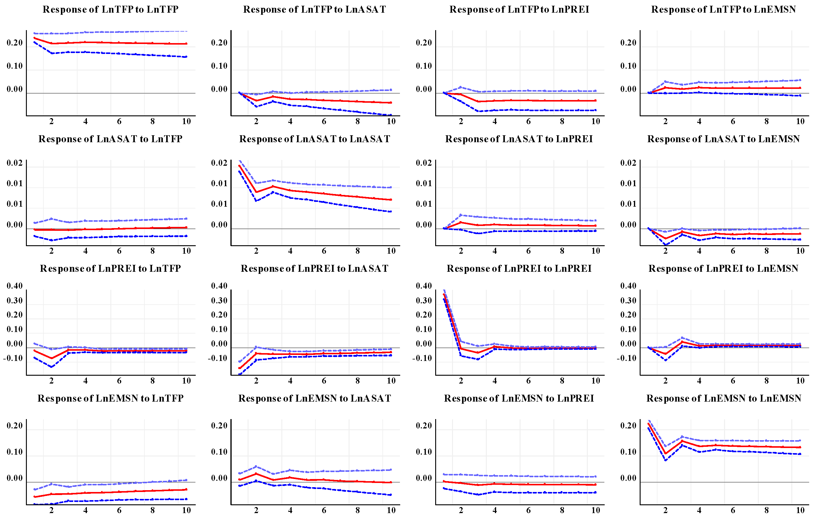
The study used IRFs to illustrate how fishery production and climate variables respond over time to a sudden shock in any one of these variables, tracing the dynamic effects of unexpected changes, showing the magnitude and duration of the response.

The IRFs from Figure 1 show that a one-standard-deviation shock to fishery production initially increases its own value by about 0.18, with the effect gradually declining to near zero by period 10, confirming strong short-run persistence. A shock to surface air temperature slightly reduces fishery production by approximately 0.02 in the first period, with the effect declining over the first 8 periods. Precipitation shocks have a minimal effect on production (less than 0.01) over all periods. Emissions initially increase fishery production by around 0.02–0.03, with the effect stabilizing by period 10.

The justifications of the initial positive response of fisheries production to emissions shocks may reflect short-run economic and environmental adjustments associated with increased emissions. However, this interpretation is unpredictable and should be viewed as a possible explanation rather than a direct inference from the model. The effect stabilizes after period 10, suggesting that the initial response reduces as longer-term environmental and economic adjustments occur.

The study results confirmed that the shocks to surface air temperature, precipitation, and emissions have temporary and modest effects, while fishery production is most sensitive to its own past values.

For FEVD results, the study defines periods 1–5 as the short run and periods 6–15 as the long run. As shown in

Table 9. Dynamic Effects of Shocks on Fishery Production and Climate Variables.

Period	Variance Decomposition of LnTFP				Variance Decomposition of LnASAT
	LnTFP	LnASAT	LnPREI	LnEMSN	LnTFP	LnASAT	LnPREI	LnEMSN
1	100.000	0.000	0.000	0.000	0.031	99.969	0.000	0.000
2	98.384	1.045	0.034	0.537	0.048	97.426	0.702	1.824
3	97.664	0.865	0.906	0.565	0.070	97.752	0.671	1.506
4	97.066	0.990	1.237	0.706	0.063	97.411	0.745	1.781
5	96.768	1.091	1.389	0.751	0.057	97.394	0.765	1.784
6	96.463	1.239	1.514	0.784	0.051	97.288	0.785	1.877
7	96.189	1.392	1.609	0.810	0.046	97.220	0.796	1.937
8	95.931	1.560	1.680	0.829	0.045	97.142	0.804	2.009
9	95.682	1.736	1.739	0.843	0.047	97.066	0.809	2.078
10	95.439	1.919	1.787	0.855	0.053	96.986	0.812	2.148
11	95.199	2.107	1.828	0.865	0.062	96.904	0.814	2.219
12	94.964	2.299	1.864	0.873	0.076	96.820	0.815	2.290
13	94.731	2.494	1.896	0.880	0.093	96.732	0.815	2.361
14	94.500	2.690	1.924	0.886	0.113	96.640	0.814	2.432
15	94.272	2.887	1.949	0.892	0.138	96.546	0.813	2.503
Period	Variance Decomposition of LnPREI				Variance Decomposition of LnEMSN
	LnTFP	LnASAT	LnPREI	LnEMSN	LnTFP	LnASAT	LnPREI	LnEMSN
1	0.332	13.296	86.372	0.000	6.102	0.159	0.014	93.724
2	3.650	13.549	81.684	1.117	7.781	1.688	0.029	90.503
3	3.688	14.329	79.979	2.004	7.710	1.294	0.138	90.858
4	3.779	15.270	78.878	2.074	7.735	1.345	0.145	90.775
5	4.014	16.184	77.612	2.190	7.647	1.188	0.163	91.002
6	4.209	16.857	76.621	2.312	7.505	1.087	0.183	91.225
7	4.399	17.493	75.676	2.431	7.332	0.980	0.201	91.488
8	4.599	18.029	74.828	2.544	7.143	0.888	0.218	91.750
9	4.799	18.496	74.051	2.653	6.946	0.811	0.236	92.008
10	5.000	18.899	73.341	2.760	6.744	0.747	0.254	92.255
11	5.202	19.246	72.688	2.864	6.542	0.699	0.271	92.488
12	5.405	19.544	72.086	2.965	6.341	0.664	0.289	92.706
13	5.608	19.800	71.529	3.063	6.144	0.643	0.307	92.906
14	5.812	20.018	71.012	3.158	5.950	0.635	0.325	93.090
15	6.014	20.204	70.531	3.251	5.762	0.640	0.343	93.255

Note: Cholesky Ordering: LnASAT, LnPREI, LnEMSN & LnTFP. Standard Errors: Monte Carlo (100 repetitions). Source: Author calculations (2026).

, short-run variations in fishery production (LnTFP) are primarily driven by own shocks, accounting for 100% in period 1 and remaining high at about 96.8% by period 5, while climate variables play a limited role, with temperature, precipitation, and emissions explaining approximately 1.1%, 1.4%, and 0.8%, respectively. In the long run, the influence of climate factors gradually increases as the contribution of LnTFP’s own shocks declines to about 94.3% by period 15, whereas temperature, precipitation, and emissions account for roughly 2.9%, 1.9%, and 0.9% of fishery production variability. Moreover, temperature and emissions remain largely self-driven in the long run, explaining over 96% and 93% of their own forecast variance, respectively, while precipitation exhibits stronger cross-variable effects, with temperature shocks contributing about 20.2% to its long-run variability.

These results are consistent with the structure of the fisheries sector, where short-run output is mainly determined by internal factors such as stock levels and harvesting capacity. Over time, climate-related shocks gradually influence production, reflecting the delayed effects of temperature, precipitation, and emissions on fishery production. The high self-dependence of temperature and emissions indicates that these variables are largely driven by broader environmental processes rather than feedback from fisheries.

4.2.3. Granger-Causality Results

Based on

Table 10. PVAR Granger Causality/Block Exogeneity Wald Tests.

Equation: LnTFP			Equation: LnASAT
Excluded	Chi2	Causality direction	Excluded	Chi2	Causality direction
LnASAT	8.407 ***	Bidirectional	LnTFP	1.389	No causality
LnPREI	4.099	Bidirectional	LnPREI	3.149	No causality
LnEMSN	3.249	Unidirectional	LnEMSN	8.936 ***	Unidirectional
ALL	15.582 ***	Joint causality	ALL	11.026 *	Not significant
Equation: LnPREI			Equation: LnEMSN
Excluded	Chi2		Excluded	Chi2	Causality direction
LnTFP	30.817 ***	Unidirectional	LnTFP	1.299	No causality
LnASAT	47.599 ***	Unidirectional	LnASAT	6.800 **	Unidirectional
LnEMSN	21.892 ***	Unidirectional	LnPREI	1.129	No causality
All	84.243 ***	Joint causality	All	8.446	Not significant

Note: ***, ** and * denote significance at 1%, 5%, and 10%, respectively. Source: Author calculations (2026).

, the results show significant causal relationships between fishery production and climate variables. LnTFP and LnASAT exhibit bidirectional causality (Chi² = 8.407, p = 0.01), while LnTFP is unidirectionally influenced by LnEMSN (Chi² = 3.249, p = 0.19) in the short run. LnPREI is strongly affected by LnTFP, LnASAT, and LnEMSN jointly (Chi² = 84.243, p < 0.01), reflecting the sensitivity of rainfall patterns to both climatic and ecological factors. For LnASAT, emissions significantly Granger-cause temperature (Chi² = 8.936, p = 0.01), while LnTFP shows no significant effect. Finally, emissions are influenced primarily by temperature (Chi² = 6.800, p = 0.03), with negligible feedback from fishery production and precipitation. Moreover, the detected causal relationship from carbon emissions to temperature reflects statistical predictability within the model rather than a direct physical long-run climate mechanism, which is driven by accumulated global emissions. Therefore, the results are interpreted with appropriate caution.

Fishery production and temperature Granger-cause each other, while precipitation responds to changes in fisheries and other climate variables. Emissions Granger-cause temperature but are largely independent of fishery production. The study shows that fishery production responds to climatic shocks, whereas climate variables are largely self-determined, with precipitation exhibiting the strongest interactions across variables.

4.3. Robustness Checks of the PVAR Model

For robustness, we employed structural residuals, endogeneity curves, and forecasting evaluation to assess the stability, reliability, and predictive performance of the PVAR model, respectively.

4.3.1. Structural Residuals Innovations of the PVAR Model

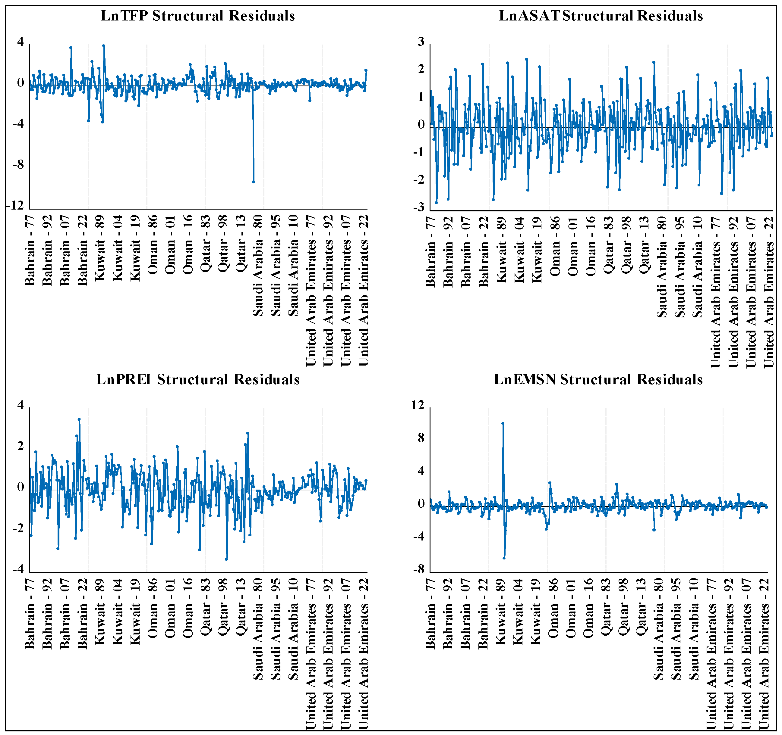
To assess the adequacy of the PVAR specification, the study analyzed the structural residuals obtained from the PVAR model using Cholesky identification with degrees-of-freedom-adjusted factors, which ensures orthogonal and uncorrelated shocks. Figure 2 illustrates that the residuals fluctuate around zero, implying that the model provides a good representation of the system’s underlying dynamics.

Fishery production shows a large negative shock around Saudi Arabia (approximately −12), indicating an unexpected decline not explained by the model. The temperature residuals fluctuate between roughly −2 and +2, reflecting moderate variability across countries. Similarly, precipitation residuals generally remain within the range of −2 to 2, with occasional spikes that may correspond to extreme rainfall events. Emissions residuals display one notable negative outlier around Kuwait (approximately −10), while most observations fall between −4 and +4, suggesting relatively stable shocks. Therefore, the residuals appear stationary and do not exhibit systematic trends, supporting the adequacy of the PVAR model in reflecting the dynamic interactions between fishery production and climate-related variables.

4.3.2. Endogenous Analysis

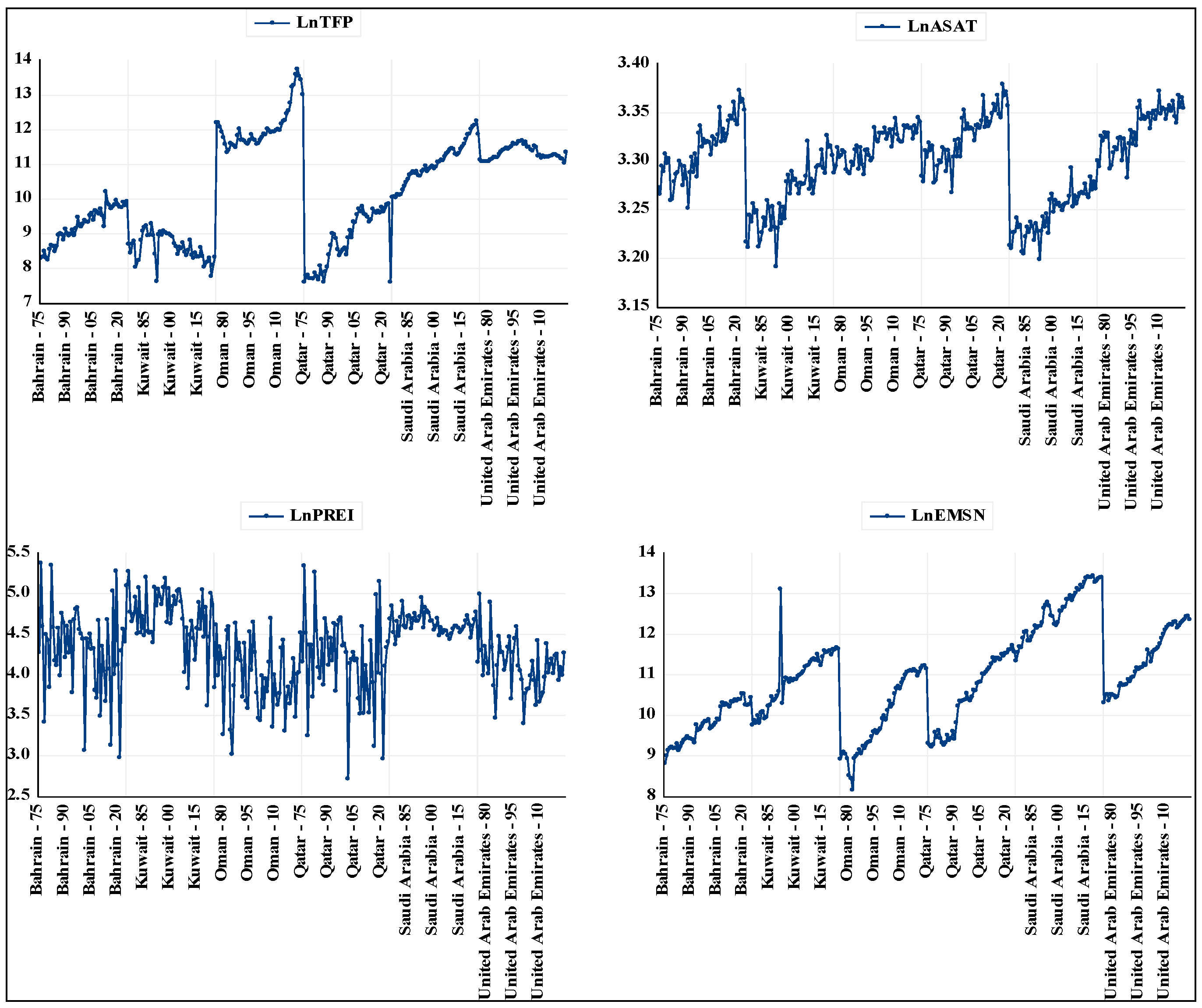
Furthermore, as a robustness check for the PVAR model, the endogenous variables were examined (Figure 3). LnTFP shows gradual growth with several fluctuations, ranging approximately from 7 to 14, reflecting variations in fishery production. LnASAT exhibits a steady upward trend from about 3.2 to 3.35, indicating gradual warming over time. LnPREI is highly volatile, fluctuating between 2.5 and 5.5, which is consistent with the irregular rainfall patterns observed in the region. LnEMSN demonstrates a clear increasing trend from around 9 to 13, reflecting the rise in emissions during the study period. These trends indicate that climate variables develop relatively smoothly over time, whereas fishery production and precipitation exhibit greater variability. This supports the PVAR model’s ability to represent the dynamic interdependencies and endogeneity among these variables.

4.3.3. Forecast Accuracy Results

Table 11. Forecast Evaluation of the selected variables.

Variable	RMSE	MAE	MAPE	Theil
LnASAT	0.017	0.013	0.396	0.003
LnEMSN	0.337	0.241	2.279	0.015
LnPREI	0.396	0.295	7.011	0.046
LnTFP	0.682	0.567	5.900	0.033

Note: RMSE: Root Mean Square Error, MAE: Mean Absolute Error, MAPE: Mean Absolute Percentage Error, and Theil: Inequality coefficient. Source: Author calculations (2026).

presents the forecast accuracy of the PVAR model for GCC countries. LnASAT has the lowest errors (RMSE = 0.017, MAE = 0.013, MAPE = 0.40%, Theil = 0.0026), indicating highly accurate predictions. LnEMSN shows moderate errors (RMSE = 0.337, MAE = 0.241, MAPE = 2.28%, Theil = 0.0154). LnPREI (precipitation) is more volatile (RMSE = 0.396, MAE = 0.295, MAPE = 7.01%, Theil = 0.046), while LnTFP exhibits the largest forecast errors (RMSE = 0.682, MAE = 0.567, MAPE = 5.90%, Theil = 0.033), reflecting higher variability. The study revealed that the model predicts climate variables more accurately than fishery and precipitation variables.

The forecast evaluation reflects inherent variability in the modeled variables. LnASAT shows very low errors because temperature trends are gradual and smooth over time, making them easier for the PVAR model to predict. LnEMSN has moderate errors due to a steady upward trend but occasional fluctuations. LnPREI and LnTFP display higher errors because these variables are naturally more volatile, as rainfall is irregular in the GCC, and fishery production is influenced by multiple unpredictable environmental and economic factors. This explains why climate variables are forecasted more accurately than fishery and precipitation variables.

5. Discussion

The empirical results confirm that fishery production in GCC countries shows strong persistence over time. There is strong cointegration between fishery production and climate change. This result is consistent with [38]. The significant first lag of fishery production indicates that current production is highly influenced by past performance, suggesting that changes in the sector occur gradually due to long production cycles, biological constraints, and institutional arrangements. The negative effect of surface air temperature on fishery production may reflect the vulnerability and the sensitivity of marine ecosystems to warming, which can reduce fish productivity and alter species distribution. This effect may be stronger in the GCC due to the Arabian Gulf’s shallow waters, high salinity, and extreme temperatures. However, since the study uses aggregate fisheries production data, it is not possible to identify specific species or fishing grounds affected. Higher temperatures reduce fish stocks and affect marine habitats, leading to lower fishery output. The study results are approved [18], showing that extremely high temperatures are expected to have net negative effects on fish stocks, leading to reduced fisheries revenues and threatening livelihoods in many maritime countries.

However, this effect declines over time, indicating that partial adjustment or adaptation may take place. These results agreed with [39], indicating that rising temperatures reduce fishery production and constrain economic development, which may indirectly affect future fisheries performance.

Precipitation has a limited and mostly insignificant effect on fishery production, which is reasonable given that GCC fisheries are primarily marine-based and less dependent on rainfall patterns. In comparison, regarding study results of other researchers, ref. [40] proved that fish yield is influenced by rainfall with a one-year lag effect. Furthermore, ref. [19] confirmed that rainfall has a negligible effect on fishery production. Emissions show delayed effects on both fishery production and climate variables, pointing to the long-term influence of industrial activity and environmental pressure on marine resources and climate conditions.

The results also show that fishery production responds strongly to climate-related shocks, particularly changes in temperature and precipitation. However, the FEVD results show that the overall contribution of climate variables to forecast error variance remains relatively small (around 6% in the long run). This suggests that while climate shocks have a statistically meaningful effect on fisheries production, the system is largely driven by its own dynamics and other non-climatic factors. Therefore, climate impacts should be interpreted as significant but limited in magnitude rather than dominant drivers of fisheries fluctuations. In contrast, temperature and emissions are mainly driven by general climate change and economic processes rather than short-term changes within the fisheries sector. Precipitation reacts to both fisheries and climate variables, indicating close links between atmospheric conditions and marine systems in the region.

The IRF results indicate that fisheries production initially responds positively to emissions shocks before stabilizing after approximately period 10. This finding may reflect short-run environmental and economic adjustments associated with climate-related changes. Previous studies have shown that climate variability can affect fish abundance, distribution, and productivity through changes in marine ecosystem conditions and primary productivity, although the direction and magnitude of these effects vary across ecosystems and species [41,42]. The subsequent stabilization of the response suggests that longer-term ecological and economic adjustments may moderate the initial effect.

The short-term positive effect of CO₂ emissions may not reflect a direct ecological benefit. Instead, CO₂ emissions are likely reflecting wider economic activity such as industrialization, energy use, and expansion of fishing capacity, which can temporarily enhance fisheries production through improved infrastructure and harvesting intensity. However, this should not be interpreted as a positive environmental outcome, as long-term effects of emissions remain associated with climate change and ocean acidification, which are generally harmful to marine ecosystems.

Large, unexpected shocks observed in fishery production in Saudi Arabia and emissions in Kuwait reflect sudden events that are not fully explained by the model. Despite these shocks, the overall stability of the residuals supports the adequacy of the PVAR specification.

Such shocks may result from policy changes, climate conditions, regulatory reforms, technological progress, or shifts in market demand. In Saudi Arabia, the rise in fisheries production from 49,000 tons in 2000 to 79,500 tons in 2022 [1] reflects structural growth rather than temporary fluctuations, likely driven by sector development programs, fleet modernization, and national initiatives such as Saudi Vision 2030 that promote food security and economic diversification.

The endogeneity analysis confirms strong interactions among all variables, indicating that none of the series evolves independently. Fishery production and precipitation show larger fluctuations, reflecting their sensitivity to short-term environmental and economic changes. By contrast, temperature and emissions change more gradually over time, which supports the treatment of all variables as endogenous within the PVAR framework. Also, we proved that temperatures and carbon dioxide emissions significantly reduce fish production.

The relatively low forecast errors for temperature and emissions reflect their stable progression over time, whereas higher errors for fishery production and precipitation reflect their greater variability and sensitivity to irregular climate conditions and economic shocks in the GCC region.

6. Conclusions

Fishery production is increasingly threatened by overfishing, climate change, marine pollution, and habitat degradation, which reduces stock regeneration and ecosystem stability. Mismanagement systems and limited technological adoption further constrain productivity. These challenges pose serious risks to food security and economic resilience, particularly in the GCC region. Therefore, this study examines the dynamic impact of climate change shocks on fishery sustainability in GCC countries. It focuses on both short- and long-run responses using a Panel Vector Autoregression (PVAR) framework and its related diagnostic techniques to investigate climate interactions.

The empirical results reveal strong dynamic links between climate factors and fishery production in GCC countries. Climate variables, particularly temperature and emissions, show stable long-term trends and are forecasted with relatively low errors, whereas precipitation and fishery production display higher variability and sensitivity to short-term shocks. The endogeneity and robustness checks confirm the relevance of the PVAR framework, showing two-way relationships among all variables. These findings highlight the need to consider climate variability when developing policies to improve fishery sustainability in the GCC region. The results also reveal significant causal links between fishery production and climate variables in the GCC, as supported by the Granger causality tests.

Also, the results confirmed that precipitation and fishery production exhibit higher forecast errors because they are inherently more volatile. Rainfall patterns are irregular in the Gulf Cooperation Council (GCC) region, while fishery output is influenced by multiple unpredictable environmental and economic factors, leading to greater variability in their forecasts.

7. Policy Implications and Study Limitations

The results suggest that fisheries policies in GCC countries should be designed with a long-term focus, as changes in fishery production occur gradually. Quick or temporary actions are unlikely to lead to meaningful improvements. Instead, continuous support for sustainable stock management and stronger institutional arrangements is required.

The negative effect of rising temperatures on fishery production highlights the need to include climate adaptation in fisheries planning. Policies should emphasize protecting marine ecosystems, improving monitoring of sea temperature and fish stocks, and promoting fishing practices that reduce pressure on sensitive species.

Given the limited influence of precipitation, policy efforts should focus on marine environmental conditions rather than rainfall-related factors. Priority should be given to addressing threats such as ocean warming, habitat degradation, and overexploitation of fish resources.

The lagged effects of emissions underline the importance of reducing environmental pressure from industrial activities. Joint environmental and climate policies among GCC countries can help protect shared marine resources and limit long-term damage. Finally, the strong links between fisheries, climate, and emissions suggest that integrated policies are needed. Coordination between fisheries, environmental, and energy authorities can improve policy outcomes and strengthen the resilience of the fisheries sector under climate uncertainty.

This study has several limitations. It uses aggregate national data, which may hide differences across regions, species, and fishing practices within GCC countries. The PVAR model assumes linear relationships and may not fully reflect nonlinear effects or extreme climate events. In addition, the analysis includes a limited set of climate variables, while other important determinants of fisheries production, such as fishing effort, overfishing intensity, fisheries management practices, and market conditions, could not be considered due to data constraints. Therefore, the estimated climate effects should be interpreted with caution, as they may partly reflect the influence of omitted factors. Furthermore, the absence of macroeconomic control variables (e.g., regional GDP or fishing capacity) may introduce omitted variable bias. Future research could incorporate such factors to improve model accuracy. Finally, the VAR framework identifies dynamic relationships but does not establish direct causal mechanisms, so the results should be interpreted with caution.