Abstract
Generic and consistent formulations for measurement of the backscattering cross section and the volume backscattering coefficient using broadband pulse compression and narrowband echo integration are derived, for small- and finite-amplitude sound propagation. The theory applies to backscattering operation of echosounders and sonars in general, with focus on fisheries acoustics. Formally consistent mathematical relationships for broadband and narrowband operation of such instruments are established that ensure consistency with the underlying power budget equations on average-power form, bridging a gap in prior literature. The formulations give full flexibility in choice of transmit signals and reference signals for pulse compression. Generic and general criteria for quantitative consistency between broadband and narrowband operation are derived, establishing new knowledge and analysis tools. These criteria become identical for small- and finite-amplitude sound propagation. In addition to general criteria, two special cases are considered, relevant for actual operation scenarios. The criteria serve to test and evaluate the extent to which the methods used in broadband pulse compression and narrowband echo integration operating modes are correct and consistent, and to identify and reduce experienced discrepancies between such methods. These are topics of major concern for quantitative acoustic stock assessment, underlying national and international fisheries quota regulations.
Keywords:
echosounder; sonar; fisheries acoustics; broadband pulse compression; narrowband echo integration; acoustic backscattering; finite-amplitude sound propagation; matched filter processing Key Contribution:
The article closes gaps in prior literature by (i) establishing generic criteria for quantitative consistency between broadband pulse compression and narrowband echo integration operation of echosounders and sonars under conditions of small- and finite-amplitude sound propagation, and (ii) by establishing formally consistent mathematical relationships for broadband and narrowband operation of such instruments that ensure consistency with the underlying power budget equations on average-power form.
1. Introduction
1.1. Background
Fisheries acoustics is of utmost importance for national and international management of marine resources, e.g., through annual allocation of quotas to the fishery fleet. Acoustic survey methods have been developed and used over decades for fish abundance estimation, typically at frequencies in the range from 20–40 kHz to 200 kHz [1,2]. Sonars designed for plankton studies generally work at higher frequencies, typically 100–5000 kHz [1,2]. Methods are being developed also for species identification, using frequencies typically in the range 20–400 kHz [3,4,5]. Methodologies in this field, including hardware and signal processing technologies, are subject to continuous development [5,6,7,8,9,10,11,12,13,14]. These methods are based on using ship-mounted scientific echosounders and sonars measuring the backscattering cross section, [units of m2], of individual targets, and the volume backscattering coefficient, [units of m−1], of assemblies of targets such as fish or plankton [2,15,16,17,18,19]. The ship-mounted echosounders are normally calibrated using a target with known , such as an elastic sphere with high characteristic acoustic impedance [20].
Traditionally, scientific fisheries echosounders and sonars are used in narrowband operation at one or several discrete frequencies (typically up to six or seven) [20] using narrowband tone bursts and echo integration methods [1,2,15,16,21,22,23]. For brevity, this approach will here be referred to as “narrowband echo integration”. Broadband methods (Appendix B.1) have been taken into use in recent years, employing pulse compression by matched filtering of modulated signals (such as linear frequency modulation) [5,6,7,8,9,10,11]. For brevity, this approach is here referred to as “broadband pulse compression”. Modern broadband echosounder systems may offer a choice between the two modes of operation, i.e., broadband pulse compression operation (often referred to as “FM mode” (Appendix B.2)), and more traditional narrowband echo integration operation (often referred to as “CW mode” (Appendix B.3)) [5,12,24,25,26].
In the following, “CW operation” and “FM operation” will be used for the two modes of operation; not as abbreviations or acronyms, but solely as short labels indicating “narrowband echo integration” and “broadband pulse compression”, respectively (Appendix B.4).
The small-amplitude power budget equations for and on average-power form [19], constituting the basis for acoustic scattering methods, are today considered well established [9,11,16,17,19,25,26,27,28,29,30,31,32,33,34,35,36,37]. Here, “average” refers to averaging of the instantaneous power over one cycle of the harmonic signal waveform [19,27,28], corresponding to the steady-state part of a transient or pulsed signal. These equations have recently been generalized to also account for finite-amplitude effects [17,32,34,38,39], for situations where high transmit powers are used and nonlinear sound propagation effects in the seawater may become significant (Appendix B.5). The equations describe the flow of time-averaged electrical and acoustic power in signal transmission, propagation, scattering, and reception [32,39,40], and they constitute the basis for both CW operation [16,17,19,27,28] and FM operation [5,9,11,25,30,35,37].
These power budget equations on average-power form cannot, however, be used directly for echosounder and sonar measurement of and . Reformulation is necessary to provide equations for operational use.
The equations may be expressed in terms of the measured voltage signals [1,2,15,19,27,28]. The two mentioned modes of operation are treated separately: (i) narrowband echo integration using tone bursts (CW operation), and (ii) broadband pulse compression using frequency modulated signals and matched filtering (FM operation). For these modes of operation to be quantitatively consistent, the power budget equations on average-power form must be transferred to both a narrowband echo integration form and a broadband pulse compression form.
For small-amplitude CW operation, several different and seemingly diverging formulations have been presented and used in different series of commonly used fisheries echosounders and sonars, such as Simrad’s EK500 [16], EK60 [23], ES60 [41], ME70 [42], MS70 [43], and Kongsberg Discovery EK80 [5,24]. Refs. [27,28] provided a unifying derivation of these, describing their consistency with the power budget equations on average-power form.
For small-amplitude FM operation, a similar derivation of a pulse compression formulation consistent with the power budget equations on average-power form is, however, not available in prior literature [37]. This unfortunate situation affects modern echosounders and sonars being operated in FM mode, such as, e.g., the widespread EK80 echosounder system [5,11,24] and others.
1.2. Research Questions
1.2.1. Consistency of CW and FM Modes of Operation
From available literature and operational experience, several questions arise. The first major question relates to the consistency of CW and FM modes of operation. As outlined in Section 1.1, in some of the new echosounder and sonar systems, one may choose between FM mode and more traditional CW mode operations [5,12,24,25,26], see Figure 1. For quantitative consistency in size and abundance measurement, it would be desirable that the CW and FM modes of operation, when used on identical targets at the same frequency, , give the same result for and , within the measurement uncertainty of each mode of operation. That is, ideally,
where superscripts FM and GW indicate the respective modes of operation being used for measurement of and .
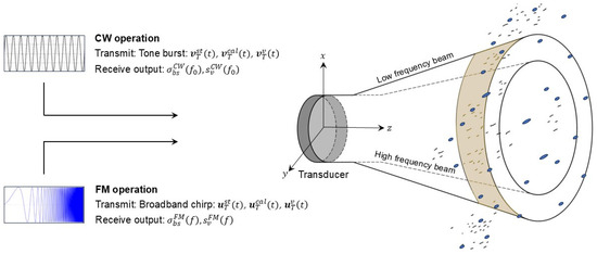
Figure 1.
Schematic illustration of CW and FM operation of an echosounder or sonar. The transducer transmits narrowband or broadband signals, respectively, and receives signals backscattered from single or multiple targets in the sea, being processed and converted to backscattering cross section () for individual targets, and volume backscattering coefficient () for assemblies of multiple targets such as fish or plankton.
From operational experiences using such echosounder systems, questions have arisen with respect to such quantitative consistency, i.e., equality of results using the CW and FM modes of operation [12,26,44,45]. This regards both (i) consistency of the theoretical functional relationships being used (i.e., the mathematical expressions), and (ii) consistency in echosounder and sonar measurement results (i.e., after being implemented in operational systems), when using the two modes of operation on the same target or fish school. The central question is: What are the criteria for Equation (1) to be fulfilled?
To enable quantitative comparison of CW and FM modes of operation, and to establish criteria for quantitative consistency between these, one should preferably know the generic (i.e., instrument-independent) and accurate functional relationships for these narrowband echo integration and broadband pulse compression measurements. These functional relationships should be based on the same calibration factor(s), so that for a given tone burst carrier frequency in CW operation, , the calibration factor and its uncertainty are eliminated in a comparison of the CW and FM modes of operation. Moreover, the functional relationships should both be consistent with the underlying power budget equations on average-power form [19,27,28]. The latter condition would ensure a consistent and traceable mathematical connection between the formulations for the CW and FM operations being used.
A derivation of a narrowband echo integration formulation consistent with the power budget equations on average-power form is already available for small-amplitude sound propagation [19,27,28]. A corresponding derivation for broadband pulse compression is, however, not available in prior literature, as pointed out by [37]. This is one of the topics addressed here, see Section 1.3.
For finite-amplitude sound propagation, the system requirements and research questions are similar: When used on identical targets, CW and FM modes of operation should ideally give the same results for and in calibration and survey measurements, within the measurement uncertainty of each mode of operation. A derivation of power budget equations on average-power form is available also for the finite-amplitude case [32]. However, neither (i) a narrowband echo integration formulation nor (ii) a broadband pulse compression formulation that is consistent with the finite-amplitude power budget equations on average-power form [32] is available in prior literature. The derivation and establishment of such formulations is also addressed here, see Section 1.3.
1.2.2. Consistency with Pulse Compression Formulations Proposed in Prior Literature
The second main research question relates to the consistency of the expressions presented here with broadband pulse compression formulations proposed in prior literature for echosounders and sonars being operated in FM mode.
Various broadband pulse compression formulations are available in the literature [5,6,7,8,9,10,11,13]. Quantitative comparison is complicated since many of these are not based on the electroacoustic average power budget equations. Due to the widespread use of the commercial Kongsberg Discovery EK80 echosounder system [24], the literature describing this system has a large impact on today’s fisheries acoustics community. As a result, the equations given in [5,11] may largely represent de facto “industry standard” power budget equations on broadband pulse compression form.
To quantitatively examine the agreement between such formulations and the average power budget equations, a first step taken herein (see Section 1.2.1 and Section 1.3) is to establish a generic functional relationship for pulse compression that is consistent with those average power budget equations [19,27,28]. A second step could be to compare the equations proposed in the prior literature to this generic pulse compression formulation. This second step is too comprehensive to be included here and is left for future work.
1.3. Objectives
The primary objective of the present work is to establish generic criteria for the consistency of CW and FM modes of operation for small- and finite-amplitude operation of scientific fishery acoustics echosounders and sonars. That is, the criteria to fulfil Equation (1).
To enable such analysis, generic functional relationships of the power budget equations for narrowband echo integration and broadband pulse compression operation will be derived. These relationships are required to be mutually consistent, and consistent with the power budget equations on average-power form [19,27,28,32]. Expressions are to be derived for single-target and multi-target (volume) backscattering measurements, in terms of and , respectively. The expressions are to account for small-amplitude and finite-amplitude sound propagation.
Generic pulse compression formulations are sought that are not only directly comparable to the corresponding generic echo integration formulations of the average power budget equations [19,32] but also with known instrument-specific echo integration formulations [23,27,28,41,42,43], so that they can be used to analyze and evaluate possible deviations or inconsistency in results between pulse compression and echo integration measurements for and . In this context, generic means instrument independent (i.e., not relying on instrument- or implementation-specific hardware or software solutions).
1.4. Alternative and Equivalent Formulations: Overview and Terminology
Table 1 gives an overview of alternative and equivalent relevant formulations for small-amplitude (linear) sound propagation. Based on the average-power formulation of the and equations given by [17,19] (denoted “Formulation ”), an echo integrator formulation has been derived for narrowband signals [28] (here denoted “Formulation ”). Based on the same “Formulation ”, a pulse compression formulation for broadband or wideband signals is derived in the present work (denoted “Formulation ”). Formulations and involve a single common instrument calibration factor, [27,28].

Table 1.
Alternative, equivalent, and consistent formulations of small-amplitude power budget equations for measurement of and (linear sound propagation). Calibration factors referred to in the table are defined in [27,28] and Section 2.2.2, Section 2.3.2, Section 3.2.2 and Section 3.3.2 (for ) and [27,28] (for , , and , see the table).
Table 2 gives an overview of the corresponding alternative and equivalent formulations for finite-amplitude (nonlinear) sound propagation. Based on the average-power formulation of the and equations given by [32] (denoted “Formulation ”), an echo integrator formulation is derived in the present work for narrowband signals (denoted “Formulation ”). Based on the same “Formulation ”, a pulse compression formulation is also derived in the present work for broadband signals (denoted “Formulation ”). Formulations and involve the same single calibration factor as Formulations and .
Table 2.
Alternative, equivalent, and consistent formulations of finite-amplitude power budget equations for measurement of and (nonlinear sound propagation).
Table 1 and Table 2 represent generalizations of Table 1 in [28] from covering small-amplitude narrowband echo integration operation only, to also cover (i) broadband pulse compression and (ii) finite-amplitude formulations of the power budget equations. Refs. [27,28] introduced the terminology “Formulations A, B, C, D, E”, adhered to here, to clarify, systemize, and differentiate between the various formulations that have been in use for different series of scientific fisheries echosounders and sonars [23,41,42,43]. Sub- and superscripts to the “formulation symbols” A, B, C, D, and E are here introduced to distinguish between CW and FM operation (subscripts “ei” for “echo integration” and “pc” for “pulse compression”) and between low-amplitude and finite-amplitude sound propagation conditions (superscript “n” indicating “nonlinear”).
The echo integration formulations , , and are addressed in [27,28] and included in Table 1 for reference. These are instrument-specific echo integration formulations applicable to the EK60, ES60, ME70, and MS70 [23,41,42,43] echosounder and sonar systems [27,28]. The differences between the generic formulation and the instrument-specific formulations , , and relate to (i) the four different approaches used for echo integration in the measurement of and , and (ii) the calibration factors used. These differences are summarized in the columns “Calibr. factors” and “Key characteristics” of Table 1. Since only generic formulations are addressed in the present work, formulations , , and , are not further discussed here.
It may be noted that, since the finite-amplitude formulations per se also cover the small-amplitude case [32], only the finite-amplitude formulations of Table 2 are strictly needed. These are however less known in the fishery acoustics community, and involve additional parameters that need to be determined (by measurement or numerical calculations) [32,34]. When significant finite-amplitude effects can be avoided, the small-signal formulations are sufficient and more convenient. For such reasons, the small- and finite-amplitude formulations are presented in separate sections.
1.5. Outline
The paper is organized as follows. Formulations for small-amplitude echosounder or sonar operation (linear sound propagation) are treated in Section 2. Section 2.1 gives a summary of the generic small-amplitude (linear) power budget equations on average-power form (Formulation A), as a basis for both the generic narrowband echo integration formulation of these equations summarized in Section 2.2 (Formulation ), and the corresponding generic broadband pulse compression formulation of these equations derived in Section 2.3 (Formulation ).
Corresponding formulations for finite-amplitude echosounder or sonar operation (nonlinear sound propagation) are treated in Section 3. Section 3.1 gives a summary of the generic finite-amplitude (nonlinear) power budget equations on average-power form (Formulation ) being used as basis for both the generic narrowband echo integration formulation of these equations derived in Section 3.2 (Formulation ), and the corresponding generic broadband pulse compression formulation of these equations derived in Section 3.3 (Formulation ).
Results are given and discussed in Section 4. Section 4.1 addresses the consistency of CW and FM modes of operation for small- and finite-amplitude conditions. Conclusions are given in Section 5. Appendix A defines the conventions and terminology used for convolution and cross-correlation in the present work.
Throughout the work, bold-face font is used for complex-valued quantities and parameters. In fisheries acoustics literature, power budget-type equations are often given in logarithmic form only [5,11,18]. For completeness and to simplify comparison with other literature, power budget-type equations are thus given both in linear and logarithmic forms here. Only generic (instrument-independent) formulations (type A and B) are addressed in this work. Instrument-dependent formulations (type C, D, E) are not addressed here, but can be treated based on the analysis given in [27,28].
The presentation of the material follows the structure of Table 1 and Table 2, by first treating small-amplitude (linear) operation (see Table 1) with presentation of formulations , , and , and then finite-amplitude (nonlinear) operation (see Table 2) with presentation of formulations , , and .
The analysis presented here makes assumptions that are common for abundance measurement in fisheries acoustics, with the exception that finite-amplitude (nonlinear) sound propagation is accounted for. The assumptions on which the analysis relies are summarized in [32].
2. Materials and Methods 1: Small-Amplitude Operation (Linear Sound Propagation)
Functional relationships describing three different but equivalent power budget formulations for small-amplitude echosounder or sonar operation (linear sound propagation) are given in the present section. These are Formulations A, , and , see Table 1.
Three different measurement situations are addressed: “single-target”, “calibration”, and “volume” backscattering. The single-target backscattering situation relates to both calibration and field operation measurements, e.g., calibration sphere and single-fish backscattering, respectively. The volume backscattering situation covers field operations with measurements on a multitude of targets, such as a fish school, krill, etc.
Transmitted voltage signal waveforms in single-target, calibration, and volume backscattering measurements are denoted , , and , respectively, where t is time. Subscript “” indicates “transmitted”. Superscripts “”, “”, and “” denote “single-target”, “single calibration target”, and “volume” backscattering, respectively.
The signal durations will normally be quite different in CW and FM modes of operation [5], since in CW operation, the total energy in the signal is concentrated at a single frequency, whereas in FM operation, the total signal energy is spread over a wide frequency band. Use of different symbols for the signal duration in the two modes of operation is thus necessary, such as to derive consistency criteria in Section 4. For CW operation, let , , and be the time durations of , , and , respectively, all starting at , the time of transmit voltage signal onset. For FM operation, let , , and be the corresponding time durations of , , and . Subscript “p” is used to indicate “ping”, commonly used for transmitted pulsed signals in the fisheries acoustics community. In CW operation, can be a typical example, corresponding to . In the EK80 echosounder system, may be set to values ranging from 0.064 to 8.192 ms [5].
Similarly, received voltage signal waveforms in single-target, calibration, and volume backscattering measurements are denoted , , and , respectively. Subscript “” indicates “received”.
For signal reception, let be the gate opening time window, where and are the start and end times of the time gate, respectively. This applies to (i) for a single-target echo ; (ii) for a calibration-target echo (e.g., a solid sphere); and (iii) for a volume scattering echo (a multitude of targets, such as a fish school). Subscript “g” denotes “gate”, used for backscattered signals.
The transmit signal waveforms , , and are measured across the transducer’s electrical terminals during transmission, after transmit electronics circuitry and components that are not embedded in the transducer itself. The received signal waveforms , , and are measured across the transducer’s electrical terminals during reception, before receiver electronics circuitry and components that are not embedded in the transducer itself.
By denoting the Fourier transform [46] of a voltage signal waveform by , one has
where is the frequency. , , , , , and are the complex-valued frequency spectra of the respective complex-valued voltage time signals in analytic form, , , , , , and , respectively.
In conventional operation, the same voltage transmit signal may often be used in single-target measurement, calibration, and volume backscatter measurement, , and the corresponding average electrical signal powers during transmission also become equal, .
For generality and flexibility, the three transmit signals are here allowed to be different. This allows study of specific scenarios like the one mentioned above, as well as other scenarios of interest.
2.1. Average-Power Formulation of Power Budget Equations (Formulation A)
In Section 2.1, a summary of the small-amplitude (linear) power budget equations on average-power form is given, taken essentially from [19,27,28], with some minor modifications in notation.
Under assumptions summarized in [19,27,28], including the assumption of small-amplitude signal propagation, the basic equations used conventionally in fish abundance estimation and species identification are
Here, harmonic time dependency has been assumed and suppressed [19], where is the angular frequency, and is time.
Equations (4) and (5) constitute the power budget equations on average-power form [19,27,28]. Physical interpretations of Equations (4) and (5) in terms of power flow are given in [27]. Equations (4) and (5) constitute Formulation A of the power budget equations for and ) [19,27,28], see Table 1. They form the basis for the narrowband echo integration formulation summarized in Section 2.2 (Formulation ), and the broadband pulse compression formulation derived in Section 2.3 (Formulation ), see Table 1. Quantities and parameters involved in Equations (4) and (5) are described in the following.
For each measurement frequency, f, in the relevant frequency band of such measurements (typically 10–500 kHz [5]), is the backscattering cross section of a single target located at position in the transducer’s far field, and is the volume backscattering coefficient for a thin far-field spherical shell (denoted “ping volume”, ) centered at the transducer front. The transducer’s far field is typically taken as ranges [47] (the Rayleigh distance), where is the effective transducer radius.
In this description, a spherical coordinate system is used with its origin centered at the face of the echosounder/sonar transducer and the direction coincident with the sound beam axis [19]. and are the polar and azimuthal angles, respectively. is the small-signal sound velocity in seawater, and is the acoustic wavelength. [units of Np/m] is the sound pressure acoustic absorption coefficient in seawater [47].
In Equation (4), r is the distance to the single target. In Equation (5), ) is the distance to the mid-range of a spherical shell, . is contained within ranges and , with spherical shell thickness [19].
and [units of W] are the average electrical transmit signal powers during transmission, for single-target and volume backscattering measurements, respectively. and [units of W] are the corresponding average electrical echo signal powers, received after two-way sound propagation, backscattering, and two-way electroacoustic transduction [19]. The respective average signal powers are given as [19,47]
Here, [units of Ω] is the transducer’s input electrical impedance at transmission when radiating into the fluid [19], and and the corresponding electrical resistance and reactance, respectively. is the output (internal) electrical impedance of the receiving transducer, and is the input electrical impedance of the connected electrical network upon signal reception. and , and and , are the respective resistances and reactances [19]. and should normally be available from the echosounder/sonar manufacturer, either as a function of frequency, or at selected frequencies in the relevant frequency range. The assumption is sometimes used if better information is not available.
and [both non-dimensional] are the transducer gain and the axial transducer gain, given as [16,17,19,48]
respectively, where [non-dimensional] is the transducer’s electroacoustic conversion efficiency (the ratio of radiated acoustic to transmitted electrical powers), and
and , are the axial directivity factor [47], the directivity factor [48], and the beam pattern [47], respectively [all non-dimensional], for the transmitted sound pressure field. Here, . and represent the transducer’s one-way electroacoustic conversion efficiency per unit solid angle, in the and axial directions, respectively, for lossless sound propagation conditions in the fluid [19,27,28].
[units of steradian, sr] is the equivalent two-way beam solid angle of the transducer, given as [16,19,48,49,50,51]
represents an effective beam width of the transducer’s intensity field, expressed in terms of a solid angle, accounting for the combined effect of transmission and reception [19,27,28]. For a given echosounder/sonar transducer, is normally provided by the echosounder/sonar manufacturer, at a selected frequency (or possibly several frequencies) in the actual frequency band of the transducer.
Finally,
are [non-dimensional] electrical termination factors for the power budget equations being formulated in terms of average power or voltage, respectively [17,19]. In the respective formulations, and account for the influence of electrical impedance load at the transducer’s terminals upon signal reception [19]. ( is not a quantity appearing in Equations (4)–(13), but will be needed in the following. It is thus considered convenient to present here, accompanying the closely related quantity .)
Equations (4) and (5) are equivalent to the expressions given in the EK500 manual [16], except for the factor which was omitted or lacking there, implicitly implying [19]. The implications of that have been discussed in [19,27,28].
Insertion of Equations (6) and (7) into Equations (4) and (5) yields
which gives the power budget equations expressed in terms of voltage spectra [28], to be used in the following. Note that in Equations (14) and (15), has taken the role of in Equations (4) and (5).
Equations (14) and (15) constitute the basis for deriving the power budget equations on echo integration and pulse compression form, see Section 2.2 and Section 2.3, respectively.
2.2. Generic Echo Integration Formulation of Power Budget Equations (Formulation )
In Section 2.2, Formulation A, through Equations (14) and (15), is developed into a generic echo integration formulation of the power budget equations (Formulation ), for comparison (in Section 4) with the generic pulse compression formulation of the power budget equations being derived in Section 2.3.
The derivation made is quite similar to the relatively detailed description given in [28], but is slightly more general here, and thus with some change in terminology, to cover independent transmit signals in single-target, calibration, and volume backscattering measurement situations that can be different, with different transmit (“ping”) durations, see Section 2.1. Details of the derivation are thus not given here; only the main results are summarized.
In the echo integration formulation, the transmit signals , , and are assumed to be tone bursts (possibly with an amplitude tapering window function) with carrier frequency . Echo integration is taken over the whole signal duration, which per se is also the steady-state part of these transmit signals, oscillating with frequency . The echo integrations of the received signals , , and with time gates , , and , respectively, are assumed to be taken over the steady-state parts of the respective received signal waveforms, oscillating with frequency . The transient start and transient end of a received signal, caused by finite system bandwidth, are thus not to be included for the echo integration to be evaluated formally correct.
2.2.1. Functional Relationship
Following the derivation given in [28], involving (i) use of Parseval’s theorem [46], , to enable processing of signals in the time domain, and (ii) time averaging of the resulting transmit and receive echo integrals, Equations (14) and (15) can be expressed in terms of echo integration, giving
where is the carrier frequency of the transmit voltage signals and , and
are the “echo integral”, or “time-integral-voltage-squared” , values of the voltage signals , , , and , respectively. (Appendix B.6, Appendix B.7)
The definition of the echo integrals given by Equations (18)–(21) corresponds to that given by [1,2,15]. The [tivs] (“time-integral-voltage-squared”) notation used here represents a generalization of the [tips] (“time-integral-pressure-squared”) notation used by Medwin and Clay [51], to account for electrical voltage instead of “in-water” sound pressure signals [19,27,28]. The echo integrals ([tivs]) represent voltage squared times seconds, in units of V2s = W·ohm·s = J·ohm [19].
Logarithmic versions of Equations (16) and (17) are obtained by dividing Equation (16) throughout with a reference area (chosen equal to 1 m2), multiplying Equation (17) throughout by a reference length (chosen equal to 1 m), and applying on both sides of Equations (16) and (17) [19,27,28], giving
respectively, where [units of dB re. ] is the target strength of a single scattering target; [units of dB re. ] is the volume backscattering strength for the “ping volume” . is the reference area for , is the reference distance for , and is a reference length for r (with , , and all chosen equal to 1 m). () [units of dB/m] is the sound pressure absorption coefficient of the fluid propagation medium [47].
Equations (16) and (17), or alternatively Equations (22) and (23), constitute a generic echo integration formulation of the power budget equations for and ), in linear and logarithmic forms, respectively.
2.2.2. Determination of Calibration Factor,
Before survey operation, at-sea calibration of the echosounder or sonar is performed. For the present echo integration formulation of the power budget equations, the calibration function to be determined is . In this approach, using a single transducer and a tone burst signal with carrier frequency , is to be determined at the frequency .
Consider a calibration situation for the echosounder or sonar using a solid calibration sphere with the sphere’s center located at position [28]. For the backscattering cross section of the sphere, a theoretical value, , is assumed known, calculated at the frequency (see e.g., [52,53,54]). Alternatively (and equivalently), the corresponding target strength may be known, for a reference area = 1 m2.
From Equation (16), can be determined from calibration measurement data as
where in use of Equation (16), superscript “st” has been replaced by “cal” to indicate calibration conditions. Here,
are the “echo integral”, or “time-integral-voltage-squared” , values of the voltage signals and , respectively. , , and are the electrical termination factor, the acoustic wavelength, and the small-signal sound speed in seawater at calibration conditions, respectively.
For the echo integration operation, quantities to be measured for determination of are , , , , , , , and . and are typically assumed to be known. In practice, calibration measurement of may be made for several sphere positions close to the acoustical axis, with subsequent averaging, for statistical improvement of the resulting calibration measurements [27,28].
Multiplying Equation (24) throughout by the factor and applying to both sides gives the logarithmic version of Equation (24),
2.2.3. “Compact” Functional Relationship
Insertion of the calibration factor from Equation (24) into Equations (16) and (17) for and ), leads to
Dividing Equation (28) throughout by the reference area , multiplying Equation (29) throughout by the factor , and applying on both sides, yields the logarithmic version of Equations (28) and (29),
Equations (28) and (29), or alternatively Equations (30) and (31), constitute the “compact” generic echo integration formulation of the power budget equations for and ), in linear and logarithmic forms, respectively. They represent generalization of the corresponding “compact” generic echo integration formulation given in [27,28], to describe transmit signals in single-target, calibration, and volume backscattering measurement situations that can all be different, and with individual transmit (“ping”) durations. This “compact” generic echo integration functional relationship is conveniently used in Section 4.1 for comparison of CW and FM modes of operation.
2.3. Generic Pulse Compression Formulation of Power Budget Equations (Formulation )
In Section 2.3, Formulation A, through Equations (14) and (15), is developed into a generic broadband pulse compression formulation of the power budget equations (Formulation ), for comparison (in Section 4) with the generic echo integration formulation of the power budget equations presented in Section 2.2.
In the pulse compression formulation, the transmit signals , , and are arbitrary, independent, and can be quite generally designed. That means, e.g., rectangular tone burst, amplitude modulated (AM) tone burst, frequency modulated (FM) signal (linear or nonlinear FM), or a combination of these. In fisheries acoustics, linear FM is often used, without AM.
2.3.1. Functional Relationship
Consider two reference voltage signal waveforms and , with which , , and are to be cross-correlated, respectively, in a matched-filtering processing procedure.
is in principle an arbitrary signal, but may in practice be either (i) the transmitted electrical voltage signal , (ii) a voltage echo signal received in pulse-echo operation using the echosounder/sonar with reflection from a solid (ideally “rigid”) wall, or (iii) a voltage echo signal received in pulse-echo operation with reflection from a calibration sphere. is also arbitrary but may in practice be (i) the transmitted electrical voltage signal , or as (ii) and (iii) above.
Note that if option (i) is used (see e.g., [5,11]), the reference signal does not account for the finite bandwidth of the transducer in transmit–receive operation. Depending on the transducer bandwidth and possible tapering window functions used, the reference signal may then be different in shape from relevant echo signals, so this is presumably the least attractive option.
If option (ii) is chosen, the reference signal does account for the transducer’s transmit and receive frequency responses and will be more similar in shape to relevant echo signals. This may appear to be the most attractive option if the same reference signal is to be used in calibration, single-target, and volume scattering applications.
If option (iii) is chosen, the reference signal accounts for the transducer’s frequency response and all “events” related to scattering from a solid sphere (e.g., the direct echo, circumferential signals, surface waves within the sphere, surface waves in the seawater, notches in the scattering spectrum due to interference between such, internal compressional-wave and shear-wave resonances, etc.). This may be thus the preferred option in a calibration situation, but presumably less relevant in survey operation.
For generality and flexibility, the general case for which the reference signals and are allowed to be arbitrary, independent, and different is considered here. This allows for and enables studies of specific scenarios like, e.g., (i)–(iii) indicated above, as well as other reference signal scenarios of relevance and interest.
In the following, let (see Appendix A)
be the frequency spectra of the respective cross-correlated signals (in the following referred to as “cross-correlation frequency spectra”), where “FT” denotes Fourier transform, the operator “” denotes cross-correlation, superscript “*” denotes complex conjugate, and
are the Fourier transforms of the respective individual signals.
In Equations (14) and (15) multiply with, respectively, (for ) and (for )) both in the numerator and denominator, leading to
respectively, where Equation (8) has been used in Equation (38). Logarithmic versions of Equations (38) and (39) are obtained as described in Section 2.2.1, giving
respectively. Equations (38) and (39), or alternatively Equations (40) and (41), constitute a generic pulse compression formulation of the power budget equations for and ), in linear and logarithmic forms, respectively.
2.3.2. Determination of Calibration Factor,
At-sea calibration of the echosounder/sonar is normally performed using one or several calibration spheres [20]. For the present pulse compression formulation of the power budget equations, the calibration function to be determined is . In this approach, using a frequency-modulated signal with matched filtering, is to be determined as a function of frequency. Different spheres may be used for different frequency bands [5].
Consider a calibration situation for the echosounder/sonar using a solid calibration sphere, with the center of the sphere located at position . From Equation (38), can be determined from calibration measurement data as
where subscript or superscript “cal” has been used to indicate calibration conditions, and
where is a reference voltage signal waveform used in the calibration situation, and
In conventional fisheries acoustics procedures for calibration of scientific echosounders or sonars, is a theoretically known (calculated) (see e.g., [52,53,54]) value for the backscattering cross section of the calibration sphere, at the frequency in question [20], see Section 2.2.2.
The logarithmic version of Equation (42) is (see Section 2.2.2)
For pulse compression operation, quantities to be measured for determination of in echosounder or sonar calibration are , , , , , , and . Similar to in CW operation (see Section 2.2.2), and are typically assumed to be known. Moreover, the calibration measurement of may in practice be performed for several sphere positions close to the acoustical axis, with subsequent averaging, for statistical improvement of the resulting calibration measurements [27,28].
2.3.3. “Compact” Functional Relationship
Insertion of (the calibration function) from Equation (42) into Equations (38) and (39) for and ) leads to
for the pulse compression formulation of the power budget equations. The corresponding expressions on logarithmic form are (see Section 2.2.3)
Equations (47) and (48), or alternatively Equations (49) and (50), constitute the “compact” generic pulse compression formulation of the power budget equations for and ), in linear and logarithmic forms, respectively. This “compact” generic pulse compression functional relationship is used in Section 4.1 for comparison of CW and FM modes of operation.
2.3.4. Special Case 1: Identical Transmit Signals; Identical Reference Signals
In pulse compression applications using scientific fisheries echosounders or sonars, the same transmit voltage signal is often used in calibration, single-target, and field operations, and a “replica” (copy) of the transmit voltage signal is used as a reference signal [5,6,7,8,9,11,55].
Consider the slightly more general situation where the same and are used in single-target survey, calibration, and volume scattering survey operations, but no replica signal is used. That is,
with the corresponding Fourier transform spectra
That is, is here not necessarily the replica of , but can be the replica. In this case, one has
giving, from Equations (47) and (48),
for the pulse compression formulation of the power budget equations, and
for this pulse compression formulation on logarithmic form.
2.3.5. Special Case 2: Identical Transmit and Reference Signals (Replica Formulation)
In pulse compression applications using scientific fisheries echosounders or sonars, a replica of the transmit voltage signal is often used as the reference signal [5,6,7,8,9,11,55]. To enable comparison, e.g., with the Kongsberg Discovery EK80 system [5,11,24], the relevant generic expressions for this scenario are of interest. Let
giving
leading to, from Equations (38) and (39),
and
for the pulse compression formulation of the power budget equations in linear and logarithmic form, respectively. Here,
are the normalized cross-correlation frequency spectra for single-target and volume backscattering, respectively.
The calibration factor can, like in Section 2.3.2, be determined from calibration measurement data as
where
have been used. The corresponding logarithmic version of Equation (74) is
Insertion of from Equation (74) into Equations (68) and (69) for and ) leads to the “compact” form of these equations, i.e.,
and
respectively, for the “compact” pulse compression formulation of the power budget equations in linear and logarithmic form.
3. Materials and Methods 2: Finite-Amplitude Operation (Nonlinear Sound Propagation)
Functional relationships generalizing the three equivalent small-amplitude power budget formulations described in Section 2 to account for finite-amplitude echosounder and sonar operation (nonlinear sound propagation in the sea) are derived in the present section. These are formulations , , and , see Table 2.
For brevity, the logarithmic expressions are omitted in Section 3. They can be derived in the same way as outlined in Section 2 for small-amplitude measurements. Expressions for the special cases 1 and 2, “Identical transmit signals; Identical reference signals” and “Identical transmit and reference signals (replica formulation)”, respectively, are not given here. They can be derived using the methods described in Section 2.3.4 and Section 2.3.5, respectively, for small-amplitude measurements.
3.1. Average-Power Formulation of Power Budget Equations (Formulation )
Generalization of Equations (4) and (5) to account for finite-amplitude sound propagation effects was proposed by [17,38] and more rigorously derived in [32]. Under assumptions summarized in [32], their form as given in [32,34] is
Equations (82) and (83) constitute the finite-amplitude (nonlinear) power budget equations on average-power form (Formulation ), see Table 2. They form the basis for the narrowband echo integration and broadband pulse compression formulations (Formulations and ) derived in Section 3.2 and Section 3.3, respectively.
In Equations (82) and (83), three factors account for finite-amplitude sound propagation effects in the measurement of and . The “axial finite-amplitude factor”, defined as [32,34]
accounts for nonlinear loss on the sound beam axis in , the sound pressure amplitude of the forward-propagating field incident on the target. is the corresponding sound pressure amplitude under assumed small-amplitude (linear) propagation conditions. Values of lies in the interval .
The “beam pattern finite-amplitude factor”, defined as [32,34]
accounts for finite-amplitude effects on the beam pattern (beam flattening) in the forward-propagating (incident) wave. and are the beam patterns of the forward-propagating pressure wave under small- and finite-amplitude sound propagation conditions, respectively. for small-amplitude (i.e., linear) sound propagation, and under finite-amplitude conditions. Since and are both unity on the sound beam axis, .
The “beam solid angle finite-amplitude factor” , defined as [32,34]
accounts for the finite-amplitude (nonlinear) loss integrated over the spherical shell in volume backscattering measurements. is the equivalent two-way beam solid angle under conditions of finite-amplitude propagation of the forward-propagating (incident) sound field.
Insertion of Equations (6) and (7) into Equations (82) and (83) yields
which expresses the finite-amplitude power budget equations in terms of voltage frequency spectra, to be used in the following. Equations (87) and (88) represent generalization of Equations (14) and (15) to cover finite-amplitude operation.
Equations (87) and (88) constitute the basis for deriving the finite-amplitude power budget equations on echo integration and pulse compression form, see Section 3.2 and Section 3.3, respectively.
3.2. Generic Echo Integration Formulation of Power Budget Equations (Formulation )
In Section 3.2, Formulation , through Equations (87) and (88), is developed into a generic echo integration formulation of the power budget equations (Formulation ), for comparison (in Section 4) with the generic pulse compression formulation of the power budget equations being derived in Section 3.3.
3.2.1. Functional Relationship
Based on Equations (87) and (88), a similar derivation as described under Section 2.2.1 and in [28] leads to the finite-amplitude power budget equations on echo integration form, at the frequency of CW operation, ,
3.2.2. Determination of Calibration Factor,
From Equation (89), a similar derivation as described under Section 2.2.2 leads to determination of the calibration factor under finite-amplitude operational conditions,
3.2.3. “Compact” Functional Relationship
Insertion of the calibration factor from Equation (91) into Equations (89) and (90) for and ), leads to
Equations (92) and (93) constitute the “compact” generic echo integration formulation of the finite-amplitude power budget equations for and ). They represent generalization of the corresponding small-amplitude equations given in Section 2.2.3 to finite-amplitude operational conditions. The “compact” generic echo integration functional relationship is used in Section 4 for comparison of CW and FM modes of operation.
3.3. Generic Pulse Compression Formulation of Power Budget Equations (Formulation )
In Section 3.3, Formulation , through Equations (87) and (88), is developed into a generic broadband pulse compression formulation of the power budget equations (Formulation ), for comparison (in Section 4) with the generic echo integration formulation of the power budget equations presented in Section 3.2.
3.3.1. Functional Relationship
On the basis of Equations (87) and (88), a similar derivation as described under Section 2.3.1 leads to the finite-amplitude power budget equations in pulse compression form,
3.3.2. Determination of Calibration Factor,
From Equation (94), a similar derivation as described under Section 2.3.2 leads to determination of the calibration factor under finite-amplitude operational conditions,
3.3.3. “Compact” Functional Relationship
Insertion of the calibration factor from Equation (96) into Equations (94) and (95) for and ), leads to
Equations (97) and (98) constitute the “compact” generic pulse compression formulation of the finite-amplitude power budget equations for and ). They represent generalization of the corresponding small-amplitude equations given in Section 2.3.3 to finite-amplitude operational conditions. The “compact” generic pulse compression functional relationship is used in Section 4 for comparison of CW and FM modes of operation.
4. Results and Discussion
4.1. Quantitative Consistency of CW and FM Modes of Operation
Let and be the measured backscattering cross section obtained using FM and CW modes of operation, respectively, and and the measured volume backscattering coefficient obtained using FM and CW modes of operation, respectively. Comparison of and can be made at a frequency of CW operation, . The same is the case for comparison of and .
Since the signal waveforms in CW and FM operation are different (typically using a tone burst at carrier frequency , and linear FM “chirp” over a given frequency band, respectively), it is necessary in a comparison of CW and FM modes of operation to distinguish between these. In this section, thus, and , etc., will be used for voltage signals and their frequency spectra in CW operation. For FM operation, the notation and , etc., will be used for voltage signals and their frequency spectra.
4.1.1. General Consistency Criteria
From Equations (28), (29), (47), and (48) (the “compact” expressions for echo integration and pulse compression under small-amplitude operational conditions), or, alternatively, from Equations (92), (93), (97), and (98) (the corresponding expressions under finite-amplitude operational conditions), one obtains, at a frequency of CW operation, ,
Equations (99) and (100) are general expressions, valid for different and independent transmit signals in single-target, calibration, and volume backscattering measurement situations. They apply to small-amplitude and finite-amplitude sound propagation conditions.
From Equations (1) and (99), a requirement of quantitative consistency between FM and CW operation in single-target backscattering, i.e., , leads to the criterion
From Equations (1) and (100), a corresponding requirement of quantitative consistency between FM and CW operation in multi-target (volume) backscattering, i.e., , yields
It is noted that in Equations (101) and (102), the right-hand sides are identical. This implies that the requirements of quantitative consistency between FM and CW operation in single-target and volume backscattering given by Equation (1), i.e., and , lead to the criterion
implying that
in which the superscripts “st”, “cal”, and “v” have been omitted, to indicate that the ratio applies to each of these three cases with the superscripts inserted, like in Equation (103). That is, for all three measurement situations, (a) single-target backscattering (individual fish, etc.), (b) solid-sphere backscattering (calibration), and (c) volume backscattering (fish school, plankton, krill, etc.), this ratio between quantities measured in FM and CW operation at signal reception and transmission, must be constant, and equal to the same constant. Equations (101) and (102) are equivalent to Equations (103) and (104).
Equation (104) states that for the consistency criterion in its most general form, the basic quantity is the ratio between (measured in FM operation) and the (measured in CW operation). For Equation (1) to be fulfilled, i.e., for consistent measurement results in FM and CW operations, the ratio of this quantity at signal reception and signal transmission, respectively, must take the same value in single-target and multi-target (volume) backscattering. That is, the ratio must be uniformly constant in all three backscattering-type measurements, i.e., it is invariant to different backscattering-type measurements.
It also appears from Equation (104) that the choices of transmit signal durations (, , ) and reception time gates (, , ) in CW operation severely affects the quantitative consistency between FM and CW operation. Such choices are thus of utmost importance to achieve consistent results in FM and CW operations, and for correct abundance estimates using CW operation (see Equations (28) and (29)).
It is noted that the comparison is to be made at a single frequency at a time—the frequency used in CW operation.
4.1.2. Special Case 1: Identical Transmit Signals; Identical Reference Signals
Equations (99) and (100) are valid for arbitrary, different, and independent transmit and reference signals in single-target, calibration, and volume backscattering measurements of the pulse compression formulation. As addressed in Section 2.3.4, a simpler approach may in practice be of interest in calibration and survey operations, referred to as “special case 1”.
Consider the simplified case that (i) in CW operation the same (arbitrary) transmit signal and pulse duration are used in single-target, calibration, and volume backscattering measurements; (ii) in FM operation, the same (arbitrary) transmit signal and pulse duration are used in single-target, calibration, and volume backscattering measurements; and that (iii) the same reference signal is used in all of these three situations. That is,
so that
Equations (99) and (100) then reduce to
respectively. From Equations (1) and (113), a requirement of quantitative consistency between FM and CW operation in single-target backscattering, i.e., , leads to the criterion
or, alternatively (and equivalently), using Equations (20) and (26),
From Equations (1) and (114), a corresponding requirement of quantitative consistency between FM and CW operation in multi-target (volume) backscattering, i.e., , leads to the criterion
or, alternatively (and equivalently), using Equations (21) and (26),
It is noted that in Equations (115)–(118), the right-hand sides are identical. This implies that the requirements of quantitative consistency between FM and CW operation in single-target and volume backscattering given by Equation (1), i.e., and , lead to the criterion
implying that
in which the superscripts “st”, “cal”, and “v” have been omitted, to indicate that the ratio applies to each of these with the superscripts inserted, as in Equation (119). That is, for all three measurement situations, (a) single-target backscattering (individual fish, etc.), (b) solid-sphere backscattering (calibration), and (c) volume backscattering (fish school, etc.), this ratio between quantities measured at signal reception is constant, and equal to the same constant. Equations (115)–(118) are equivalent to Equations (119) and (120).
Equation (120) states that for the consistency criterion of this special case 1, the basic quantity is the ratio of (measured in FM operation) to the (measured in CW operation). For Equation (1) to be fulfilled, i.e., for consistent measurement results in FM and CW operations, this quantity is to be evaluated for signal reception only. That is, for signal reception, this quantity must take the same value in single-target and multi-target (volume) backscattering. The quantity is thus to be invariant to different backscattering types of measurement.
For the current special case 1, the consistency criterion given by Equation (120) may appear rather different from the general consistency criterion, given by Equation (104). This is not the case. The reason is that under the assumptions given by Equations (105)–(107), Equation (104) simplifies considerably, reducing to Equation (120).
4.1.3. Special Case 2: Identical Transmit and Reference Signals (Replica Formulation)
Consider the special case 2 discussed in Section 2.3.5, whereby in FM operation, the reference signal is equal to the transmit signal for each of the measurement situations single-target, calibration, and volume backscattering measurements (replica formulation). That is,
so that
Equations (99) and (100) then reduce to
From Equations (1) and (126), a requirement of quantitative consistency between FM and CW operation in single-target backscattering, i.e., , leads to the criterion
From Equations (1) and (127), a corresponding requirement of quantitative consistency between FM and CW operation in multi-target (volume) backscattering, i.e., , yields
In Equations (128) and (129), the right-hand sides are identical. This implies that the requirements of quantitative consistency between FM and CW operation in single-target and volume backscattering given by Equation (1), i.e., and , lead to the criterion
implying that
in which the superscripts “st”, “cal”, and “v” have been omitted, to indicate that the ratio applies to each of these with the superscripts inserted, as in Equation (130). That is, for all three measurement situations, (a) single-target backscattering (individual fish, etc.), (b) solid-sphere backscattering (calibration), and (c) volume backscattering (fish school, etc.), this ratio between quantities measured at signal reception and transmission, must be constant, and equal to the same constant. Equations (128) and (129) are equivalent to Equations (130) and (131).
Equation (131) states that for the consistency criterion of this special case 2, the basic quantity is the ratio of (measured in FM operation) to the (measured in CW operation). For Equation (1) to be fulfilled, i.e., for consistent measurement results in FM and CW operations, the ratio of this quantity at signal reception and signal transmission, respectively, must take the same value in single-target and multi-target (volume) backscattering. That is, this ratio is to be invariant to different backscattering types of measurement.
For the current special case 2, the consistency criterion given by Equation (131) is quite similar to the general consistency criterion, given by Equation (104). The only difference is in the numerator of the basic quantity referred to above, i.e., involving instead of . The reason is that under the assumptions given by Equation (121), Equation (104) simplifies somewhat, reducing to Equation (131).
Table 3 summarizes the main results of the work: Equation (104) [the generic consistency criterion for Equation (1) to be valid], Equation (120) [the corresponding consistency criterion for Special case 1], and Equation (131) [the corresponding consistency criterion for Special case 2], together with the respective underlying assumptions stated in the derivations. These criteria apply to small- as well as finite-amplitude sound propagation.
Table 3.
Summary of the main results of the work.
5. Conclusions
Generic and consistent formulations for measurement of the backscattering cross section and the volume backscattering coefficient using broadband pulse compression (“FM operation”) and narrowband echo integration (“CW operation”) are derived, for small- and finite-amplitude sound propagation in use of scientific echosounders and sonars.
The article bridges gaps in prior literature by (i) establishing generic criteria for quantitative consistency between FM and CW operation of echosounders and sonars under conditions of small- and finite-amplitude sound propagation, and (ii) by establishing formally consistent mathematical relationships for FM and CW operation of such instruments that ensures consistency with the underlying power budget equations on average-power form.
In the present description, formulations for CW and FM operation of fisheries echosounders and sonars are sought that give full flexibility in choice of transmit and reference signals, to cover a wide spectrum of applications and methods, and to enable optimization of calibration and survey measurements. For CW operation, the description allows independent and different transmit signals , , and in single-target, calibration, and volume backscattering operation. This includes different transmit signal durations , , and for the respective three cases. Similarly, for FM operation, the description allows arbitrary, independent, and different transmit signals , , and in single-target, calibration, and volume backscattering operation. The description also allows for arbitrary reference signals , , and in such operations.
In relation to operational scenarios used in practice, two simplified special cases 1 and 2 are also considered: (1) “Identical transmit signals; Identical reference signals”, and (2) “Identical transmit and reference signals (replica formulation)”.
General and generic criteria for quantitative consistency between broadband pulse compression (FM operation) and narrowband echo integration (CW operation) of echosounders and sonars are derived, for in single-target backscattering and for in volume backscattering. Criteria for quantitative consistency of FM and CW operation of echosounders and sonars do not appear to have been available in relevant literature; the present analysis thus serves to bridge a gap in this respect, and to establish new knowledge and analysis tools. The criteria are based on the requirements and in single-target and volume backscattering operations, respectively, where superscripts “FM” and “CW” indicate FM and CW operation. It is noted that the criteria derived here can be used at single frequencies only (i.e., at a single frequency at a time); at the carrier frequency used in CW operation. Criteria are derived for the general case, and the two simplified special cases 1 and 2. It is shown that the criteria become identical for small-amplitude (linear) and finite-amplitude (nonlinear) sound propagation.
The general consistency criterion given by Equation (104) states that for all three measurement situations, (a) single-target backscattering (individual fish, etc.), (b) solid-sphere backscattering (calibration), and (c) volume backscattering (fish school, plankton, krill, etc.), a certain ratio between quantities measured in FM and CW operation at signal reception and transmission, is uniformly constant. That is, the ratio is invariant to the three considered types of backscattering measurement. For the special cases 1 and 2, the criterion simplifies, given by Equations (120) and (131), respectively.
The criteria derived here can be used to test, analyze, and evaluate the extent to which the methods and implementations for FM and CW operation of fisheries echosounders and sonars are correct and consistent. Through such analysis, the criteria may enable the identification of and reduction in experienced deviations between results from FM and CW operation of such instruments. The expressions presented establish generic functional relationships as a platform to reduce measurement uncertainty in fisheries acoustics, and to further develop and standardize echosounder and sonar calibration. The criteria may also be useful for evaluation of pulse compression, matched filtering, and signal processing strategies in fisheries acoustics, in relation to calibration and survey operation.
Apart from the issue of quantitative consistency between FM and CW operation addressed above, it is of course implicitly understood that for abundance estimation to be quantitatively correct, the complete expressions for and must be used. That means accounting for all parts of these expressions that are not included in the echosounder calibration quantity being used.
Through the results presented, a basis is established to analyze and evaluate deviations between governing equations presented and used in prior literature on FM operation in fisheries acoustics. For application of the criteria to commercial instruments [5,11], instrument-specific formulations and expressions (for and ), methods, and technical solutions may have to be accounted for. Only generic formulations are treated in this work. Corresponding instrument-specific formulations may be derived on basis of the descriptions given here and in, e.g., [27,28].
The theory described here applies to fisheries acoustics as well as backscattering operation of echosounders and sonars in general, operated at small-amplitude or finite-amplitude conditions with respect to sound propagation in the fluid medium at hand.
Author Contributions
The objectives, theory, and resulting quantitative consistency criteria were developed by P.L., and A.O.P. contributed with experience from fisheries research calibration, and measurement and numerical calculation of finite-amplitude (nonlinear) effects in fisheries acoustics. Both authors contributed to the assembly and writing of the paper. All authors have read and agreed to the published version of the manuscript.
Funding
The work was made under the CRIMAC Centre for Research-Based Innovation, funded by the Research Council of Norway (grant no. 309512) and the Centre partners.
Institutional Review Board Statement
Not applicable.
Data Availability Statement
The original contributions presented in this study are included in the article. Further inquiries can be directed to the corresponding author.
Acknowledgments
The CRIMAC Centre for Research-Based Innovation is acknowledged (https://www.hi.no/en/hi/forskning/projects/crimac).
Conflicts of Interest
The authors declare no conflicts of interest. The funder and the Centre partners had no role in the design of the study; in the collection, analyses, or interpretation of data; in the writing of the manuscript, or in the decision to publish the results.
Appendix A. Convolution and Cross-Correlation Terminology and Relationships
Since varying correlation terminology is used in the literature, with different definitions of the cross-correlation function used in different textbooks (see e.g., [46,47,49,51,56,57]), the terminology and definitions used here are included and specified, for clarity and precision. For two complex-valued time signals and the convolution of these is defined as [56]
where the operator “*” denotes convolution. For cross-correlation of complex-valued time signals, the following definition is used [56,57] (consistent with [46,47] for real-valued signals),
where superscript “*” denotes a complex conjugate. In matched filtering type of pulse compression, is the received signal and is a “copy” of the expected signal [57], often referred to as the replica signal. Often, the transmitted voltage signal is used for . Here, is arbitrary and independent of the transmit signal, and will be referred to as the “reference signal”, to provide greater flexibility in the options available for in pulse compression scenarios.
The following Fourier theorems apply for convolution and cross-correlation, respectively [56],
where and are the Fourier transforms of and , respectively, and and are the Fourier transforms of and .
Appendix B
Appendix B.1
According to [9] the term “broadband” often refers to a “system that uses FM transmit signals and hardware capable of transmitting and receiving over a range of frequencies”, and the term “wideband” often refers to a “system that combines multiple transducers, each with different broadband or narrowband signals and capabilities, to span a range of frequencies larger than can be achieved with a single transducer”. This distinction is not used here; “broadband” is taken to cover both.
Appendix B.2
In general, “FM” is an abbreviation for “frequency modulation”. In fisheries acoustics, the term “FM mode” has been rather established since, typically, linear frequency modulated signals are being used, combined with cross-correlation signal processing
Appendix B.3
In general, “CW” is an abbreviation for “continuous wave”, denoting a monofrequency signal. By some authors, “CW” is also used for a narrowband tone burst excited using a single carrier frequency, denoted “CW pulse” [58]. In fisheries acoustics, this latter terminology has been common [5]. Use of a “CW pulse” combined with echo integration signal processing is often denoted “CW operation” or “CW mode”
Appendix B.4
For example, the “FM” tag is not meant to impose limitations with respect to signals used in broadband pulse compression operation. Broadband and narrowband signals, subject to arbitrary amplitude, frequency, and phase modulations, can all be described in terms of the “broadband pulse compression” theory presented here. With respect to the pulse compression signal processing, cross-correlation is presumed [57].
Appendix B.5
Formally, “small amplitude” means “infinitely small amplitude”, since sound propagation is always nonlinear (subject to finite-amplitude effects), and linear sound propagation is formally valid only in the limit of zero amplitude. In practice, finite-amplitude effects may be negligible for small and moderate amplitudes, depending on factors including the type of propagation medium (gas, fluid, solid) and its physical properties, the requirements of measurement accuracy, electronics, acoustic transducer properties, etc. In the context of fisheries acoustics, the determination and quantification of the voltage and sound pressure amplitude levels for which finite-amplitude effects become important for the accuracy of abundance estimation and species determination is a field of ongoing research, see e.g., [5,13,14,17,26,32,34,38,39]. There are today not sufficiently established quantitative limits for which a signal can be assumed to be “small” in such applications, but theory, numerical methods and software, and measurement methods are now becoming available to systematically investigate this topic [17,32,34,38,39].
Appendix B.6
It may be noted that “echo integral” is written here using quotation marks, since the waveforms , , and appearing in the respective Equations (18), (19), and (25) are not echo signals, but transmit signals. It is convenient to use the same “echo integral” terminology for all of Equations (18)–(21) and Equations (25) and (26).
Appendix B.7
By some authors (see e.g., [2,15,22,50]), a term “echo-integrator equation” has been used to describe the range integration of the volume backscattering coefficient, , to obtain the area backscattering coefficient, , where the latter range integral is given, e.g., in [19] [see Equations (1) and (51)–(54) in [19]]. Such very close terminology may cause confusion. The “echo-integrator equation” is not addressed in the present work, and the term “echo integration” is here used solely in the meaning of Equations (18)–(21) and (25)–(26), in agreement with the terminology used by [1,2,15].
References
- MacLennan, D.; Simmonds, E. Fisheries Acoustics; Chapman & Hall: London, UK, 1992. [Google Scholar]
- Simmonds, J.; MacLennan, D.N. Fisheries Acoustics: Theory and Practice, 2nd ed.; Blackwell Science Ltd.: Oxford, UK, 2005. [Google Scholar]
- Zakharia, M.E.; Magand, F.; Hetroit, F.; Diner, N. Wideband sounder for fish species identification at sea. ICES J. Mar. Sci. 1996, 53, 203–208. [Google Scholar] [CrossRef]
- Korneliussen, R.J.; Diner, N.; Ona, E.; Berger, L.; Fernandes, P.G. Proposals for the collection of multifrequency acoustic data. ICES J. Mar. Sci. 2008, 65, 982–994. [Google Scholar] [CrossRef]
- Demer, D.A.; Andersen, L.N.; Bassett, C.; Berger, L.; Chu, D.; Condiotty, J.; Cutter, G.R., Jr.; Hutton, B.; Korneliussen, R.; Le Bouffant, N.; et al. 2016 USA—Norway EK80 Workshop Report: Evaluation of a Wideband Echosounder for Fisheries and Marine Ecosystem Science, ICES Cooperative Research Report No. 336; Int. Council for Exploration of the Sea (ICES): Copenhagen, Denmark, 2017; 79p. [Google Scholar]
- Stanton, T.K.; Chu, D. Calibration of broadband active acoustic systems using a single standard spherical target. J. Acoust. Soc. Am. 2008, 124, 128–136. [Google Scholar] [CrossRef]
- Stanton, T.K.; Chu, D.; Jech, J.M.; Irish, J.D. New broadband methods for resonance classification and high-resolution imagery of fish with swimbladders using a modified commercial broadband echosounder. ICES J. Mar. Sci. 2010, 67, 365–378. [Google Scholar] [CrossRef]
- Lavery, A.C.; Chu, D.; Moum, J.N. Measurements of acoustic scattering from zooplankton and oceanic microstructure using a broadband echosounder. ICES J. Mar. Sci. 2010, 67, 379–394. [Google Scholar] [CrossRef]
- Lavery, A.C.; Bassett, C.; Lawson, G.L.; Jech, J. Exploiting signal processing approaches for broad-band echosounders. ICES J. Mar. Sci. 2017, 4, 2262–2275. [Google Scholar] [CrossRef]
- Bassett, C.; Lavery, A.C.; Maksym, T.; Wilkinson, J.P. Laboratory measurements of high-frequency, acoustic broadband backscattering from sea ice and crude oil. J. Acoust. Soc. Am. 2015, 137, EL32–EL38. [Google Scholar] [CrossRef]
- Andersen, L.N.; Chu, D.; Handegard, N.O.; Heimvoll, H.; Korneliussen, R.; Macaulay, G.J.; Ona, E.; Patel, R.; Pedersen, G. Quantitative processing of broadband data as implemented in a scientific split-beam echosounder. Methods Ecol. Evol. 2023, 15, 317–328. [Google Scholar] [CrossRef]
- Levine, R.; de Robertis, A.; Bassett, C. Comparable estimates of volume scattering from narrowband and broadband echosounder signals. Presentation given at ICES/CIEM WGFAST Working Group on Fisheries Acoustics Science and Technology. Plouzané, France, 9–12 April 2024. [Google Scholar]
- Khodabandeloo, B.; Ona, E.; Macaulay, G.J.; Korneliussen, K. Nonlinear crosstalk in broadband multi-channel echosounders. J. Acoust. Soc. Am. 2021, 149, 87–101. [Google Scholar] [CrossRef]
- Khodabandeloo, B.; Pedersen, G.; Forland, T.N.; Korneliussen, K. Pulse duration, frequency band, and sweep direction effects on crosstalk in wideband backscattering measurements. J. Acoust. Soc. Am. 2024, 156, 391–404. [Google Scholar] [CrossRef]
- MacLennan, D.N. Acoustical measurements of fish abundance. J. Acoust. Soc. Am. 1990, 87, 1–15. [Google Scholar] [CrossRef]
- Simrad, A.S. Operator Manual: SIMRAD EK500 Fishery Research Echo Sounder. Scientific Echo Sounder: Base Version. Doc. no. P2170/Rev. G.; Simrad AS (now Kongsberg Discovery AS): Horten, Norway, 1997. [Google Scholar]
- Pedersen, A. Effects of Nonlinear Sound Propagation in Fisheries Research. PhD Thesis, University of Bergen, Bergen, Norway, 2007. [Google Scholar]
- Ona, E.; Mazauric, V.; Andersen, L. Calibration methods for two scientific multibeam systems. ICES J. Mar. Sci. 2009, 66, 1326–1334. [Google Scholar] [CrossRef]
- Lunde, P.; Pedersen, A.O.; Korneliussen, R.J.; Tichy, F.E.; Nes, H. Power-Budget and Echo-Integrator Equations for Fish Abundance Estimation; Fisken og Havet no. 10/2013; Institute of Marine Research: Bergen, Norway, 2013; 39p. [Google Scholar]
- Demer, D.A.; Berger, L.; Bernasconi, M.; Bethke, E.; Boswell, K.; Chu, D.; Domokos, R.; Dunford, A.; Fässler, S.; Gauthier, S.; et al. Calibration of Acoustic Instruments; ICES Cooperative Research Report No. 326; International Council for Exploration of the Sea (ICES): Copenhagen, Denmark, 2015; 136p. [Google Scholar]
- Dragesund, O.; Olsen, S. On the possibility of estimating year-class strength by measuring echo abundance of 0-group fish. Fiskeridirektoratets Skrifter, Serie Havundersøkelser 1965, 13, 48–75. [Google Scholar]
- Dalen, J.; Nakken, O. On the application of the echo integration method. ICES Document CM 1983/B:19; Int. Council for Exploration of the Sea (ICES), Copenhagen, Denmark. 1983, 19, 30p. [Google Scholar]
- Simrad EK60; Scientific Echo Sounder. Reference Manual. Release 2.4.X. Doc. no. 164692/Rev. D. Simrad AS (Now Kongsberg Discovery AS): Horten, Norway, 2012.
- Kongsberg Discovery EK80; EK80 Reference Manual. Wide Band Scientific Echo Sounder. Reference manual. 25.2.x, Document 395234/L. Kongsberg Discovery AS: Horten, Norway, 2025; 648p.
- Berges, B.; van de Sande, J.; Quesson, B.; Sakinan, S.; van Helmond, E.; van Heijningen, A.; Burggraaf, A.; Fassler, S. Practical Implementation of Real-Time Fish Classification from Acoustic Broadband Echo Sounder Data; Res. Rep. C076/19; Wageningen University and Research: Wageningen, The Netherlands, 2019; 151p. [Google Scholar]
- De Robertis, A.; Bassett, C.; Andersen; Wangen, L.N.I.; Furnish, S.; Levine, M. Amplifier linearity accounts for discrepancies in echo-integration measurements from two widely used echosounders. ICES J. Mar. Sci. 2019, 76, 1882–1892. [Google Scholar] [CrossRef]
- Lunde, P.; Korneliussen, R.J. A Unifying Theory Explaining Different Power Budget Formulations Used in Modern Scientific Echosounders for Fish Abundance Estimation; Fisken og Havet no. 74/2014; Institute of Marine Research: Bergen, Norway, 2014; 32p. [Google Scholar]
- Lunde, P.; Korneliussen, R.J. Power-budget equations and calibration factors for fish abundance estimation using scientific echo sounder and sonar systems. J. Mar. Sci. Eng. 2016, 4, 43. [Google Scholar] [CrossRef]
- Macaulay, G.J.; Vatnehol, S.; Gammelsæter, O.B.; Peña, H.; Ona, E. Practical calibration of ship-mounted omni-directional fisheries sonars. Methods Oceanogr. 2016, 17, 206–220. [Google Scholar] [CrossRef]
- Jech, J.M.; Lawson, G.L.; Lavery, A.C. Wideband (15–260 kHz) acoustic volume backscattering spectra of Northern krill (Meganyctiphanes norvegica) and butterfish (Peprilus triacanthus). ICES J. Mar. Sci. 2017, 74, 2249–2261. [Google Scholar] [CrossRef][Green Version]
- Berges, B.; Sakinan, S.; Berg, S.; Lusseau, S.M.; Schaber, M.; O’Connnel, S. HERAS Survey Indices: Automation, TAF and Testing; CVO Rep. 21.007; Wageningen University and Research: Wageningen, The Netherlands, 2021; 52p. [Google Scholar]
- Lunde, P. Finite-amplitude power budget equations for acoustic fish abundance estimation. J. Mar. Sci. Eng. 2020, 8, 98. [Google Scholar] [CrossRef]
- Furusawa, M. Volume scattering and echo integration in fisheries acoustics revisited. J. Mar. Sci. Technol. 2021, 29, 109–120. [Google Scholar] [CrossRef]
- Pedersen, A.O.; Lunde, P.; Korneliussen, R.J.; Tichy, F.E. Finite-amplitude sound propagation effects in volume backscattering measurements for fish abundance estimation. Acta Acust. 2022, 6, 14. [Google Scholar] [CrossRef]
- Loranger, S.; Jech, M.J.; Lavery, A.C. Broadband acoustic quantification of mixed biological aggregations at the New England shelf break. J. Acoust. Soc. Am. 2022, 152, 2319–2335. [Google Scholar] [CrossRef] [PubMed]
- Cutter, G.R.J.; Reis, C.S.; Nylund, S.; Watters, G.M. Antarctic krill biomass and flux measured using wideband echosounders and acoustic doppler current profilers on submerged moorings. Front. Mar. Sci. 2022, 9, 784469. [Google Scholar] [CrossRef]
- Ai, Q.; Li, H.; Yao, J.; Li, C.; Tao, J. Broadband scattering characteristic quantization technique for single fish based on a split-beam echosounder. Fishes 2024, 9, 12. [Google Scholar] [CrossRef]
- Lunde, P.; Pedersen, A.O. Sonar and power budget equations for backscattering of finite amplitude sound waves, with implications in fishery acoustics for abundance estimation of marine resources. In Proceedings of the 35th Scand. Symp. Physical Acoustics, Geilo, Norway, 29 January–1 February 2012; 11p. [Google Scholar]
- Lunde, P. Equations describing finite-amplitude effects in acoustic fish abundance estimation. J. Acoust. Soc. Am. 2015, 138 (Suppl. S3), 1949. [Google Scholar] [CrossRef]
- Lunde, P.; Pedersen, A.O. Volume backscattering of finite-amplitude acoustic waves: Power flow, sampled volume, and scattering cross section. In Proceedings of the 38th Scandinavian Symposium on Physical Acoustics, Geilo, Norway, 1–4 February 2015; 3p. [Google Scholar]
- Simrad ES60; Fish Finding Echo Sounder Reference Manual. Doc. no. 857-160970/Rev.H. Simrad AS (Now Kongsberg Discovery AS): Horten, Norway, 2006.
- Simrad ME70; Scientific Multibeam Echo Sounder Reference Manual. Release 1.2.5. Doc. no. 328588/Rev. B. Simrad AS (Now Kongsberg Discovery AS): Horten, Norway, 2012.
- Simrad MS70; Scientific Multibeam Sonar. Operator Manual. Doc. no. 301088/Rev. C. Simrad AS (Now Kongsberg Discovery AS): Horten, Norway, 2007.
- Rautureau, C.; Goulon, C.; Guillard, J. In situ TS detections using two generations of echo-sounder, EK60 and EK80: The continuity of fishery acoustic data in lakes. Fish. Res. 2022, 249, 106237. [Google Scholar] [CrossRef]
- Pedersen, G.; Korneliussen, R.J. Personal Communication; Institute of Marine Research: Bergen, Norway, 2023–2024. [Google Scholar]
- Brigham, E.O. The Fast Fourier Transform and its Applications; Prentice-Hall: London, UK, 1988. [Google Scholar]
- Kinsler, L.E.; Frey, A.R.; Coppens, A.B.; Sanders, J.V. Fundamentals of Acoustics, 4th ed.; John Wiley & Sons: New York, NY, USA, 2000. [Google Scholar]
- Balanis, C. Antenna Theory: Analysis and Design, 3rd ed.; John Wiley & Sons: Hoboken, NJ, USA, 2005. [Google Scholar]
- Clay, C.S.; Medwin, H. Acoustical Oceanography: Principles and Applications; John Wiley & Sons: New York, NY, USA, 1977; pp. 438–449. [Google Scholar]
- Foote, K.G.; Vestnes, G.; MacLennan, D.; Simmonds, E. Calibration of Acoustic Instruments for Fish Density Estimation: A Practical Guide; ICES Cooperative Research Report No. 144; International Council for Exploration of the Sea (ICES): Copenhagen, Denmark, 1987; 81p. [Google Scholar]
- Medwin, H.; Clay, C. Fundamentals of Acoustical Oceanography; Academic Press: Boston, MA, USA, 1998. [Google Scholar]
- Faran, J.J. Sound scattering by solid cylinders and spheres. J. Acoust. Soc. Am. 1951, 23, 405–418. [Google Scholar] [CrossRef]
- Hickling, R. Analysis of echoes from a solid elastic sphere in water. J. Acoust. Soc. Am. 1962, 34, 1582–1592. [Google Scholar] [CrossRef]
- MacLennan, D.N. The theory of solid spheres as sonar calibration targets. Scott. Fish. Res. Rep. 1981, 22, 18p. [Google Scholar]
- Chu, D.; Stanton, T.K. Application of pulse compression techniques to broadband acoustic scattering by live individual zooplankton. J. Acoust. Soc. Am. 1998, 104, 39–55. [Google Scholar] [CrossRef]
- Burdic, W.S. Underwater Acoustic System Analysis; Prentice-Hall: Hoboken, NJ, USA, 1984; pp. 219–226. [Google Scholar]
- Lurton, X. An Introduction to Underwater Acoustics Principles and Applications, 2nd ed.; Springer: Berlin/Heidelberg, Germany; Praxis Publishing: Chichester, UK, 2010; pp. 231–232, pp. 246–247. [Google Scholar]
- Abraham, D.A. Underwater Acoustic Signal Processing. Modeling Detection and Estimation; ASA Press: Ultimo, Australia; Springer: Cham, Switzerland, 2019; p. 13. [Google Scholar]
Disclaimer/Publisher’s Note: The statements, opinions and data contained in all publications are solely those of the individual author(s) and contributor(s) and not of MDPI and/or the editor(s). MDPI and/or the editor(s) disclaim responsibility for any injury to people or property resulting from any ideas, methods, instructions or products referred to in the content. |
© 2025 by the authors. Licensee MDPI, Basel, Switzerland. This article is an open access article distributed under the terms and conditions of the Creative Commons Attribution (CC BY) license (https://creativecommons.org/licenses/by/4.0/).