Fish Biomass Estimation Under Occluded Features: A Framework Combining Imputation and Regression

Abstract

In biomass estimation based on size-related features, regression models are commonly used to predict fish mass. However, in real-world scenarios, fish are often partially occluded by others, resulting in missing or corrupted features. To address this issue, we propose a robust framework that integrates feature imputation with regression. Missing features are first reconstructed through imputation, followed by regression for biomass prediction. We evaluated various imputation and regression methods and found that the autoencoder achieved the best performance in imputation. Among regression models, SVR, Extra Trees, and MLP performed best in their respective categories. These three models, combined with the autoencoder, were selected to construct the final framework. Experimental results demonstrate that the proposed framework significantly improves performance. For instance, the RMSE of SVR, Extra Trees, and MLP decreased from 21.10 g, 2.49 g, and 18.40 g to 6.53 g, 1.95 g, and 5.09 g, respectively.

1. Introduction

Precision aquaculture involves the application of control-engineering principles to enhance production by improving farmers’ ability to monitor, control, and document biological processes in fish farms [1]. A key objective of this approach is to enable more autonomous and continuous biomass monitoring [2], as fish biomass serves as a reliable indicator of both fish condition and ecosystem health [3]. Accurate biomass estimation allows for nonintrusive assessment through a variety of methods, such as acoustic or hydroacoustic monitoring [4,5], environmental DNA (eDNA) analysis [6,7,8], and computer vision techniques [9,10].

Acoustic and hydroacoustic monitoring are widely used for large-scale biomass estimation, but they lack precision in determining the exact weight of individual fish. The accuracy of acoustic-based biomass estimation is affected by various biological and physical factors, such as the small physical size of the fauna, mixed aggregations, swimbladder regression, resonance, effects of depth, ontogenetic decreases in fish body density, non-linear conversion of scattering strength to weight, and biases of the gear used for ground-truthing [11]. Additionally, the diel vertical migration (DVM) of Antarctic krill (Euphausia superba) can greatly bias the results of qualitative and quantitative hydroacoustic surveys, which are conducted with a down-looking sonar [12], highlighting a key limitation caused by biological behavior. Similarly, environmental DNA (eDNA) methods are also influenced by biological and environmental conditions. eDNA detectability declines with time after the species source is removed [13] and degrades faster at higher temperatures [14]. These complex, dynamic factors make accurate modeling challenging for both acoustic and eDNA-based assessments.

Fish farmers need to have information about individual fish features such as length, weight, sex, maturity and skin colour during different growth stages to monitor growth status for better stock management [15]. Computer vision technology offers a significant advantage in this regard by enabling the extraction of such individual-level data. For biomass estimation, computer vision primarily supports three key applications: fish mass measurement, counting, and direct biomass estimation [10,16].

Given the strong correlation between fish biometric features (height, length, and width) and weight [17], mass estimation methods based on these features offer high interpretability. For instance, ref. [18] employed binocular stereo vision combined with DL-YOLO (a YOLOv5-based model) to measure individual fish size, then applied a linear model for length-weight estimation and a power model for height-weight estimation. Similarly, ref. [19] segmented fish images and extracted features such as area and perimeter via a PCA and CF method, which were then fed into Multilayer Perceptron (MLP) [20] for fish mass prediction. In another study, ref. [11] employed 3D mesh reconstruction to derive volumetric measurements that were subsequently correlated with biomass. Despite methodological differences, these approaches share a common strategy: estimating mass through regression models applied to features extracted from a preliminary model. As such, size-based methods demonstrate effective performance in mass estimation.

A substantial number of efficient regression algorithms have been proposed in the literature [21,22]. However, the majority of these methods implicitly assume that missing data do not affect the analysis of datasets [23]. In reality, missing data is a common issue in scientific research [24], and its presence can lead to multiple complications, including performance degradation, challenges in data analysis, and biased outcomes caused by discrepancies between missing and complete values [25]. Therefore, in practical applications, it is essential either to develop robust regression models that can yield reliable results despite missing data or to design effective strategies for handling missing values.

Traditional parametric models (e.g., linear models, exponential models, and polynomial models) are generally inadequate for handling missing values, leading to unstable predictions when features are absent, since each feature contributes to the model. Due to these limitations, we focus our evaluation on machine learning approaches that demonstrate superior capabilities in modeling complex nonlinear relationships while providing inherent robustness to missing values, noise, and outliers. The selected models include Support Vector Regression (SVR) [26], K-Nearest Neighbor (KNN) [27], and Classification and Regression Trees (CART) [28], all of which offer flexible nonlinear modeling capabilities. Among ensemble learning models, we consider bagging-based approaches, including Random Forest [29] and Extremely Randomized Trees (Extra Trees) [30], as well as boosting-based models such as Gradient Boosting Decision Tree (GBDT) [31], and CatBoost [32]. We also include neural network-based approaches such as the MLP and TabNet [33], which combines neural networks with boosting-style sequential attention mechanisms. These advanced techniques simplify feature selection and interaction mechanisms compared with traditional parametric methods while making no assumptions about data distributions. This comprehensive selection of methods provides robust alternatives to conventional parametric approaches, particularly in scenarios involving incomplete data or complex feature relationships. To facilitate visualization of the high-dimensional hyperparameter spaces, we computed the Euclidean distance between each candidate and the optimal configuration, as shown in Figure 1.

In order to address the issue of feature missingness in biomass estimation, a framework was proposed that integrates imputation and regression. Within this framework, missing features are first reconstructed through the process of imputation, followed by regression to estimate the target variable. The imputation step assists in restoring the data to a more complete form, thereby enhancing the accuracy of prediction.

Hence, the objectives of the present study were fourfold:

(1) Application-Oriented Regression Framework. To propose a practical regression framework tailored for real-world scenarios, particularly addressing the issue of feature occlusion in computer vision applications, and demonstrating its effectiveness through experimental validation.

(2) Hyperparameter Optimization. To identify the optimal hyperparameter combinations for various regression models trained on the full set of 32 features from the perch dataset (representing individual perch).

(3) Feature Missingness Simulation. To develop and apply a uniform sampling strategy for simulating feature missingness, allowing the systematic evaluation of model behavior under incomplete data.

(4) Model Stability Analysis. To propose an evaluation method based on cross-validation and evaluation metrics for assessing model robustness across varying degrees of feature missingness.

2. Materials and Methods

In this study, in order to regress fish weights based on size features, data spanning various growth stages were selected for analysis. The relationships between different features were examined, and a uniform sampling strategy was applied to simulate missing data patterns. Furthermore, to systematically compare and evaluate existing regression models, a series of evaluation metrics was proposed. Subsequently, the models exhibiting optimal robustness and predictive performance were selected based on grid search and comprehensive evaluation.

2.1. Data Acquisition

We obtained perch (Lateolabrax maculatus) data from the Fujian MINWELL Industrial Co., Ltd, Fuding, China. The collected samples spanned a wide weight range (23.09 g to 757.49 g), representing multiple growth stages. After capture, all fish were anesthetized to ensure accurate morphological measurements. The dataset included a total of 125 samples, comprising 94 from healthy individuals and 31 from diseased individuals. For each sample, we measured its mass, along with 12 traditional morphometric features and 20 geometric morphometric features derived from 11 anatomical landmarks, as detailed in Figure 2. A strong positive Spearman correlation was observed among these size-based features, as shown in Figure 3. All features were normalized using standard scaling, by subtracting the mean and dividing by the standard deviation.

To verify the similarity between healthy and diseased fish distributions, we performed the Maximum Mean Discrepancy (MMD) test [34]. The results (p = 0.3291) indicated no significant difference between the two groups, confirming good distributional similarity. Therefore, subsequent experiments do not differentiate between healthy and diseased fish.

In practice, size-based features may be absent due to occlusion. To simulate such conditions, we applied a masking procedure to the dataset. It was important to note that the missingness caused by occlusion was completely random and independent of other features. Therefore, we assumed that the missing data mechanism followed the Missing Completely At Random (MCAR) pattern.

Given the limited size of our dataset, we adopted a data augmentation strategy to mitigate this constraint by sampling multiple valid features for each sample while ensuring uniform expansion across all samples. Specifically, suppose the original feature set F contains n features. For the i-th sample, we randomly sample m features from F without replacement, and repeat this process T times. As a result, each original sample yields T augmented instances with different subsets of features. This approach effectively expands the dataset size from N to at least $N\times T$, where N is the number of original samples.

$$F_i^{\left(t\right)}\subset F,\left|F_i^{\left(t\right)}\right|=m,\forall i\in \{1,\dots ,N\},\forall t\in \{1,\dots ,T\}$$

(1)

where $F_i^{\left(t\right)}$ denotes the subset of features sampled in the t-th iteration for sample i. This method addresses the issue of limited sample size by generating diverse training examples from the available data.

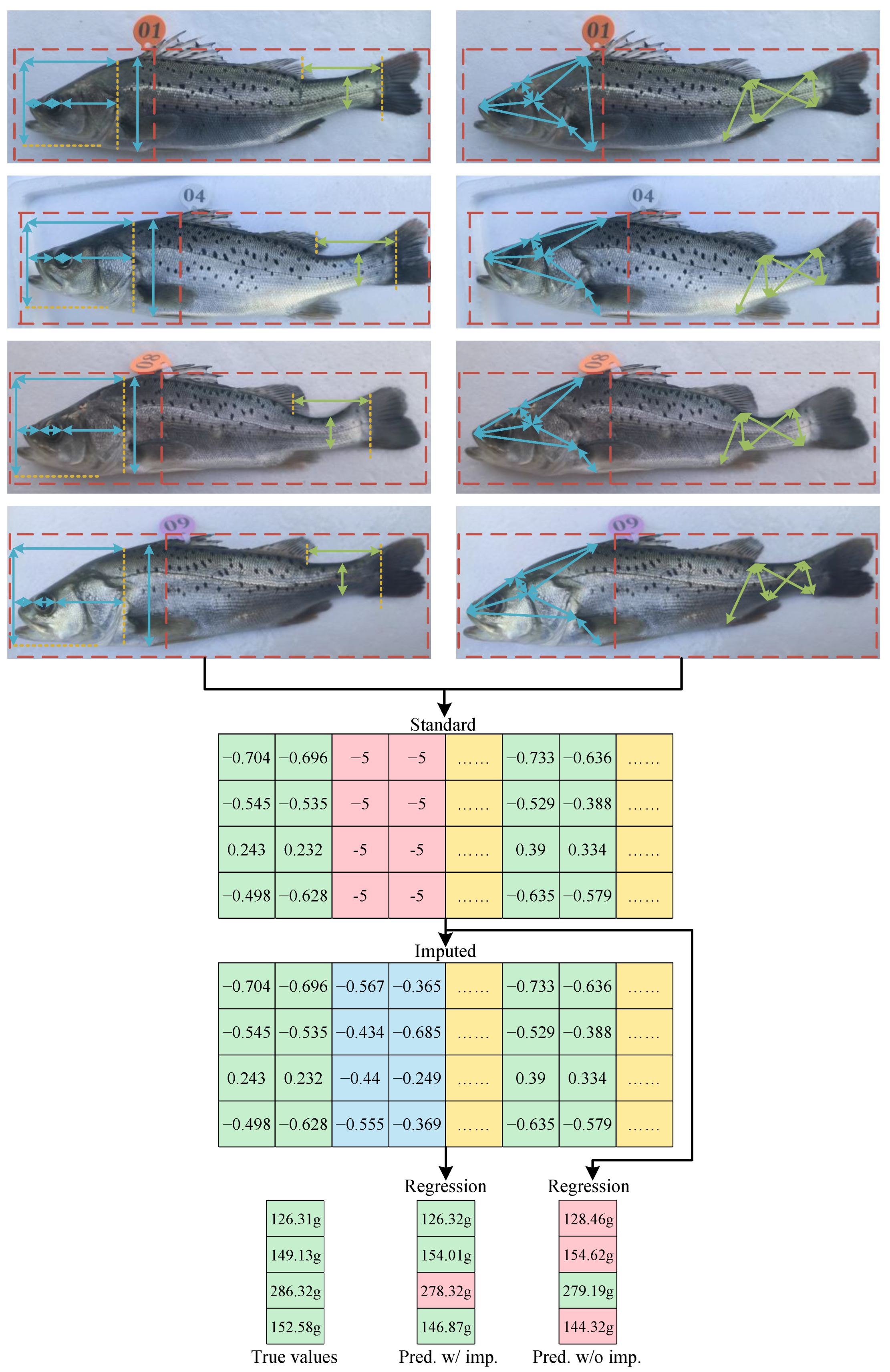
2.2. Overview of the Imputation-Regression Framework

Missing data is a common problem faced by researchers and data scientists. Machine learning-based imputation methods are gaining popularity due to their applicability and effectiveness in handling large datasets [35].

In this study, we propose an imputation-regression framework tailored for regression tasks based on size-related features. While fish biomass can be estimated from partial length measurements, these features are frequently incomplete due to various real-world factors, which limit the direct application of regression models. To address this, the framework employs imputation techniques to reconstruct missing features from the available observed data, thereby approximating the original feature values. This approach provides a generalizable solution for predictive tasks relying on size-based features, enabling more accurate biomass estimation despite missing information.

Moreover, our framework is cross-species applicable, as it relies on size-based features that are commonly shared among different fish species. The predictive accuracy primarily depends on the quality of these features. Therefore, if feature measurements obtained through computer vision (CV) techniques contain significant errors, such as those caused by image distortion, the performance of the framework could be considerably affected.

In summary, the effectiveness of this framework depends on the capacity of the imputation methods to sufficiently reconstruct missing features and the capability of the regression model to achieve accurate prediction performance.

2.3. Masking and Imputation

To simulate varying levels of occlusion, we adopted the feature reservation strategy described in Section 2.1. This process not only expands the dataset but also introduces partial feature loss. The proportion of retained features was controlled by the reservation ratio r ($0<r<1$), which will be detailed later. Importantly, this region-specific masking strategy, designed from the perspective of individual samples, more accurately reflects the real-world occlusion effects commonly observed in computer vision-based fish monitoring.

To address the feature missingness, we evaluated three representative imputation techniques: mean imputation (baseline), KNN imputation [36] and autoencoder imputation. KNN imputation was selected based on prior research [37], which demonstrated its superior performance compared with alternative methods, including mean imputation, median imputation, predictive mean matching, Bayesian Linear Regression, Linear Regression, non-Bayesian, and Random Sampling. Additionally, we adopted autoencoder imputation, which is used in prior work [38,39], where missing values are reconstructed through an encoder-decoder framework. The structure of our autoencoder is illustrated in Figure 4, with the channel dimensions explicitly indicated for each layer. It is a tiny network, comprising only 54,528 parameters and requiring 54.53K FLOPs in total.

The imputation methods were evaluated under three representative feature reservation ratios, $r\in \{0.2,0.5,0.8\}$, corresponding to the square root, 50%, and 80% of the total number of features, respectively. These settings were chosen to systematically assess the effectiveness of imputation techniques under varying levels of available information, thereby identifying the most suitable method for our task.

2.4. Regression Models

Three categories of models were employed in this study: single models, tree-based methods, and neural networks. Each category exhibits distinct characteristics in terms of robustness and sensitivity to missing data.

Single models, including SVR and KNN, were used as baseline controls. These models are generally unstable, as they are sensitive to small perturbations in the training data. Nevertheless, they demonstrate limited resilience to outliers. In particular, KNN is highly susceptible to performance degradation under feature missingness, as the distance-based neighbor selection becomes unreliable when input features are incomplete.

Tree-based models, including CART, Random Forest, Extra Trees, GBDT, and CatBoost, offer greater robustness. With the exception of CART, these models are ensemble learning methods that leverage either bagging [40] or boosting [41] strategies. Both of them are among the best-known perturbation and combination (P&C) methods. These techniques are general strategies for improving prediction rules [42], where the enhancement of predictive performance is achieved by aggregating multiple weak learners—typically decision trees—each trained on varied data subsets or weighted samples.

Bootstrap aggregation (e.g., Random Forest, Extra Trees), or bagging, is a technique that can be used with many regression methods to reduce the variance associated with prediction, and thereby improve the prediction process [42]. Bagging takes advantage of the instability by training the models using random samples (with replacement) of the dataset, named bootstrap samples [43]. The instability of the base learners was utilized, and the accuracy of the ensemble was enhanced through aggregation.

Boosting (e.g., GBDT, CatBoost), like bagging, is a committee-based approach that can be used to improve the accuracy of classification or regression methods [42]. While boosting generally enhances accuracy, its performance can degrade under missing data conditions, as early-stage errors may be amplified by incomplete information.

Neural networks, represented here by MLP and TabNet, inherently support feature fusion through fully connected layers or attention mechanisms, providing a degree of robustness to missing data. In MLP, missing inputs suppress the activation of corresponding hidden layer units, thereby implicitly balancing the output of the model. TabNet introduces soft feature selection with controllable sparsity. This sequential feature selection strategy enhances model interpretability. However, this mechanism lacks explicit attention to feature missingness—missing features can still be selected and subsequently influence the prediction. In brief, the absence of effective attention to feature missingness can result in the misleading selection of important features. Overall, the structural design of neural networks effectively mitigates the impact of missing features, providing inherent robustness.

To facilitate implementation, most models—including SVR, KNN, CART, MLP, Random Forest, Extra Trees, and GBDT were implemented using the scikit-learn library [20]. CatBoost was provided by [32], and TabNet was constructed using the open-source implementation by [33].

2.5. Hyperparameter Grid Search

A comprehensive grid search was conducted prior to simulating feature missingness to identify the optimal model configurations. The hyperparameter space was constructed by taking the Cartesian product of all individual hyperparameter sets. The performance of each model was evaluated using K-fold cross-validation, employing three standard regression metrics: Root Mean Squared Error (RMSE), Mean Absolute Error (MAE), and the coefficient of determination $R^2$, as detailed in Section 2.6.

The grid search method was applied to all the models described in Section 2.4. Hyperparameter ranges were primarily determined based on recommendations from the official library implementations of each model. For structural hyperparameters, such as network architecture or sampling strategy, values were fixed prior to grid search based on empirical insights, as detailed in the subsequent settings.

To ensure real-time performance and computational efficiency, the search space for complex models were limited. Specifically, the order of magnitude of the grid was restricted to ${10}^3$. Unless otherwise specified, all models used the default hyperparameter settings provided by their respective libraries.

In addition, for each model, the hyperparameter space was compressed by computing the Euclidean distance (denoted g) between the best-performing hyperparameters and all others after Z-score normalization. It should be noted that the hyperparameters were originally sampled on either logarithmic or linear scales. Therefore, prior to normalization, the hyperparameters were transformed back to their original scales by applying the inverse transformation in order to mitigate the influence of scaling.

For SVR, the radial basis function (RBF) kernel was adopted. A grid search was conducted over three hyperparameters: the regularization parameter $C\in \{{10}^{-3},{10}^{-2}\}$, the epsilon-insensitive margin $ϵ=0.02k$, where $k\in \{1,2,\dots ,10\}$, and the kernel coefficient $\gamma \in \{{10}^{-4},{10}^{-3},\dots ,10\}$.

Regarding KNN regression, the brute-force search algorithm was adopted due to its suitability for sparse input data. A uniform weighting scheme was used, and equal weight was assigned to all neighbors. The number of neighbors was selected from the range $n_k\in 1,2,\dots ,30$, and the power parameter for the Minkowski metric p was selected between Manhattan distance ($p=1$) and Euclidean distance ($p=2$).

The tree-based models, namely CART, Random Forest, Extra Trees and GBDT, shared a common set of hyperparameters, including the maximum tree depth d, minimum samples required to split an internal node $s_s$, minimum samples required to be at a leaf node $s_l$, and the number of features to consider when looking for the best split $n_f$. All models employed the squared error as the splitting criterion to ensure equivalence in optimization methods across both tree-based and neural network models.

Specifically for CART, the random split strategy was utilized to choose the split at each node, as it is more robust to randomly missing features. Grid search was carried out over the following ranges: $d\in \{2,4,\dots ,10\}$, $s_s$ set equal to d, $s_l\in \{3,4,\dots ,10\}$, and $n_f\in \{0.2,0.4,\dots ,1.0\}$.

With respect to Random Forest and Extra Trees, an additional hyperparameter, the number of estimators $n_e$, was introduced. The grid search covered: $n_e\in \{50,100,\dots ,500\}$, $d\in \{2,4,\dots ,10\}$, $s_s\in \{2,5,\dots ,8\}$, $s_l$ set equal to $s_s$, and $n_f\in \{0.2,0.4,\dots ,1.0\}$.

In the case of GBDT, two additional hyperparameters were incorporated: the learning rate $l_r\in \{{10}^{-3},{10}^{-2}\}$ which shrinks the contribution of each tree, and the subsample ratio $s\in \{0.5,0.7,1.0\}$, representing the fraction of samples to be used for fitting the individual base learners. In addition to these, the grid search for others spanned: $n_e\in \{100,200,\dots ,500\}$, $d\in \{3,6,9\}$, $s_s\in \{2,5,8\}$, $s_l$ set equal to $s_s$, and $n_f\in \{0.2,0.6,\dots ,1.8\}$.

As for CatBoost, the RMSE loss function was used. Bayesian bootstrap was used to mitigate sampling bias, while the Lossguide strategy was adopted to guide tree growth based on RMSE minimization, thereby improving predictive accuracy. The learning rate was fixed at $l_r={10}^{-2}$. The grid search was performed over the following: number of boosting iterations $n_i\in \{100,200,\dots ,500\}$, tree depth $d\in \{3,6,9\}$, minimum number of training samples in leaf $n_l\in \{2,5,8\}$, subsample ratio of columns $s_r\in \{0.2,0.6,1.0\}$, coefficient at the $L_2$ regularization term of the cost function $c\in \{1,2,3\}$ and bagging temperature $t\in \{0.5,1.0,\dots ,2.0\}$, which controls the intensity of Bayesian bagging.

With regard to MLP, Adaptive Moment Estimation (Adam) was adopted as the optimizer, with a constant learning rate applied across epochs. The network consisted of two hidden layers, each followed by a batch normalization layer (BN) and a ReLU activation function. Grid search was performed over the following: the width of each hidden layer $w_i=32k$, where $k\in \{1,2,\dots ,8\}$ and i denotes the index of the hidden layer, the learning rate $l_r\in \{{10}^{-4},{10}^{-3},{10}^{-2}\}$, the strength of the $L_2$ regularization term $\alpha \in \{{10}^{-4},{10}^{-3}\}$.

In the context of TabNet, the number of independent Gated Linear Units (GLUs) per step was fixed at 2, as was the number of shared GLUs. The model was trained using the Adam optimizer, with MSE as the loss function. To prevent overfitting, all models were trained with early stopping, with a maximum of 100 epochs. Grid search was conducted over the following hyperparameters: the dimension of the prediction layer $n_d=4k+8$, where $k\in \{0,1,\dots ,6\}$, the dimension of the attention layer $n_a\in \{4,6,8,10\}$, the number of successive steps $n_s\in \{3,6,9\}$, the scaling factor for attention updates $\gamma \in \{1.0,1.3,1.5,1.8,2.0\}$, and the learning rate $l_r\in \{{10}^{-3},{10}^{-2}\}$.

As shown in Figure 5, the optimal hyperparameters for each model were selected based on the lowest RMSE obtained from 10-fold cross-validation. The complete grid search results for all models are summarized in

Table 1. Summary of hyperparameter grid search across models. “Dim.” indicates the number of hyperparameter dimensions. “Params” lists the corresponding hyperparameters. “Grid” refers to the total number of hyperparameter combinations evaluated. “Score” represents the mean RMSE. “Time” is the average time per grid point. “Train” is the total training time (with “nan” indicating negligible duration). All results are based on 10-fold cross-validation. The bold number indicates the best performance of each indicator.

Model	Dim.	Params	Grid	Score	Time (s)	Train (h)
SVR [26]	3	$C,ϵ,\gamma$	360	20.10	0.15	0.01
KNN [27]	2	$n_k,p$	60	25.47	0.15	nan
CART [28]	4	$d,s_s,s_l,n_f$	1000	38.41 ± 4.53	0.14	0.04
Random Forest [29]	5	$n_e,d,s_s,s_l,n_f$	2250	26.19 ± 0.45	4.55	2.79
Extra Trees [30]	5	$n_e,d,s_s,s_l,n_f$	2250	21.92 ± 0.25	2.63	1.56
GBDT [31]	7	$n_e,d,s_s,s_l,n_f,l_r,s$	2430	22.17 ± 0.31	4.01	2.62
CatBoost [32]	6	$n_i,d,n_l,s_r,c,t$	2160	23.71	9.41	5.65
MLP [20]	4	$w_1,w_2,l_r,\alpha$	384	23.71 ± 2.08	2.06	0.22
TabNet [33]	5	$n_d,n_a,n_s,\gamma ,l_r$	840	28.84	102.64	23.95

. Several regions in the hyperparameter space display locally smooth and gradually improving performance, attributed to the fact that wider spacing between hyperparameter values does not cause significant increases in RMSE. In contrast, distinct discontinuity regions, often referred to as performance cliffs, are also observed—where minor changes in hyperparameter values lead to sudden and significant increases in RMSE. This is particularly evident in tree-based models. These findings highlight the sensitivity of model performance to specific hyperparameter configurations.

2.6. Evaluation Metrics

To evaluate model performance under feature missingness, we introduced a novel stability evaluation method. This assessment considers both the stability and predictive performance of each model across varying levels of feature availability, which are controlled by the reservation ratio r, defined as follows:

$$r={\displaystyle \frac{m}{n}}$$

(2)

where n denotes the total number of features and m represents the number of features retained (i.e., not masked) per sample. A higher r implies less feature missingness and, consequently, more complete input information.

For each reservation ratio r, we performed K-folds cross-validation. The mean RMSE across all folds was used as the cross-validation performance score, denoted as ${\overline{E}}_r$. To evaluate the stability of each model, the coefficient of validation across all folds was used. They are defined as follows:

$$\begin{array}{cc}\hfill & \overline{E_r}={\displaystyle \frac{1}{K}}\sum _{i=1}^K{E}_{r,i}\hfill \\ \hfill & {\sigma }_r^2={\displaystyle \frac{1}{K}}\sum _{i=1}^K{(E_{r,i}-\overline{E_r})}^2\hfill \\ \hfill & c_r={\displaystyle \frac{{\sigma }_r}{\overline{E_r}}}\hfill \end{array}$$

(3)

where $E_{r,i}$ denotes the RMSE for i-th fold, ${\sigma }_r$ is the standard deviation, and $c_r$ reflects the variability across folds, under reservation ratio r. A lower $c_r$ indicates greater model stability under feature-missing conditions.

In addition to RMSE, we also employed MAE and $R^2$ as an aid to evaluate model accuracy. The metrics are defined as follows:

$$\begin{array}{cc}\hfill & \mathrm{RMSE}=\sqrt{{\displaystyle \frac{1}{n}}\sum {({\widehat{y}}_i-y_i)}^2}\hfill \\ \hfill & \mathrm{MAE}={\displaystyle \frac{1}{n}}\sum \left|{\widehat{y}}_i-y_i\right|\hfill \\ \hfill & R^2=1-{\displaystyle \frac{\sum {(y_i-{\widehat{y}}_i)}^2}{\sum {(y_i-\overline{y})}^2}}\hfill \end{array}$$

(4)

where ${\widehat{y}}_i$ is the predicted mass value, $y_i$ is the ground truth, and $\overline{y}$ is the mean of the true mass values.

To evaluate imputation performance, we first compute the Normalized Root Mean Square Error (NRMSE) for each feature and then calculate the mean NRMSE across all features. The formulas are as follows:

$$\begin{array}{cc}\hfill & {\mathrm{NRMSE}}_j={\displaystyle \frac{\sqrt{\frac{1}{n}\sum {({\tilde{x}}_{ij}-x_{ij})}^2}}{max\left(x_j\right)-min\left(x_j\right)}}\hfill \\ \hfill & \overline{\mathrm{NRMSE}}={\displaystyle \frac{1}{n}}{\mathrm{NRMSE}}_j\hfill \end{array}$$

(5)

where ${\tilde{x}}_{ij}$ is the imputed value for the j-th feature of the i-th sample, $x_{ij}$ is the ground truth value, and n is the total number of features. The lower the mean NRMSE value, the better the estimate of the missing values.

3. Results and Discussion

3.1. Model Performance Without Feature Missingness

We first evaluated the predictive performance of each model under the complete feature set, using optimized hyperparameters derived from grid search (configurations shown in Figure 5). The evaluation results, with both true and predicted values inverse-transformed (a process that would be applied to all subsequent experiments), for both 5-fold and 10-fold cross-validation, are summarized in

Table 2. The performance of each model was evaluated over 10 repeated experiments, using both 5-fold and 10-fold cross-validation. Performance metrics, including RMSE, MAE, and $R^2$ are reported as the mean values averaged across all folds. The bold number indicates the best performance of each indicator.

Model	5-Fold			10-Fold
	RMSE	MAE	${\mathit{R}}^{\mathbf{2}}$	RMSE	MAE	${\mathit{R}}^{\mathbf{2}}$
SVR [26]	23.22	14.98	0.98	20.10	13.75	0.98
KNN [27]	30.88	18.53	0.96	25.47	16.04	0.97
CART [28]	39.54 ± 4.21	26.30 ± 2.62	0.94 ± 0.02	38.41 ± 4.53	25.59 ± 2.68	0.93 ± 0.02
Random Forest [29]	28.51 ± 0.44	17.66 ± 0.26	0.97	26.19 ± 0.45	16.91 ± 0.26	0.97
Extra Trees [30]	23.98 ± 0.62	14.97 ± 0.35	0.98	21.92 ± 0.25	14.34 ± 0.23	0.98
GBDT [31]	24.50 ± 0.53	15.32 ± 0.36	0.98	22.17 ± 0.31	14.47 ± 0.22	0.98
CatBoost [32]	25.76	16.55	0.98	23.71	15.85	0.98
MLP [20]	26.99 ± 1.97	17.26 ± 0.86	0.97 ± 0.01	23.71 ± 2.08	17.05 ± 1.38	0.97 ± 0.01
TabNet [33]	40.73	31.21	0.92	28.84	23.76	0.96

. Overall, 10-fold cross-validation generally yielded better performance compared with 5-fold. This can be attributed to two factors: the hyperparameters were tuned specifically under 10-fold validation, and each fold in 10-fold uses a larger training proportion (90% vs. 80%), which improves generalization and reduces underfitting risk. The performance gap between the two settings, measured in terms of RMSE, ranged from 2.86% to 17.87%, which is within an acceptable range and suggests that all models exhibited stable performance across different validation strategies.

SVR achieved the best overall performance on our dataset, offering both strong accuracy and computational efficiency due to its simple structure. Among tree-based models, Extra Trees performed comparably to SVR. In contrast, TabNet exhibited highly unstable results, which cannot be attributed to a limited hyperparameter search space. The underlying causes are further discussed in Section 3.2.

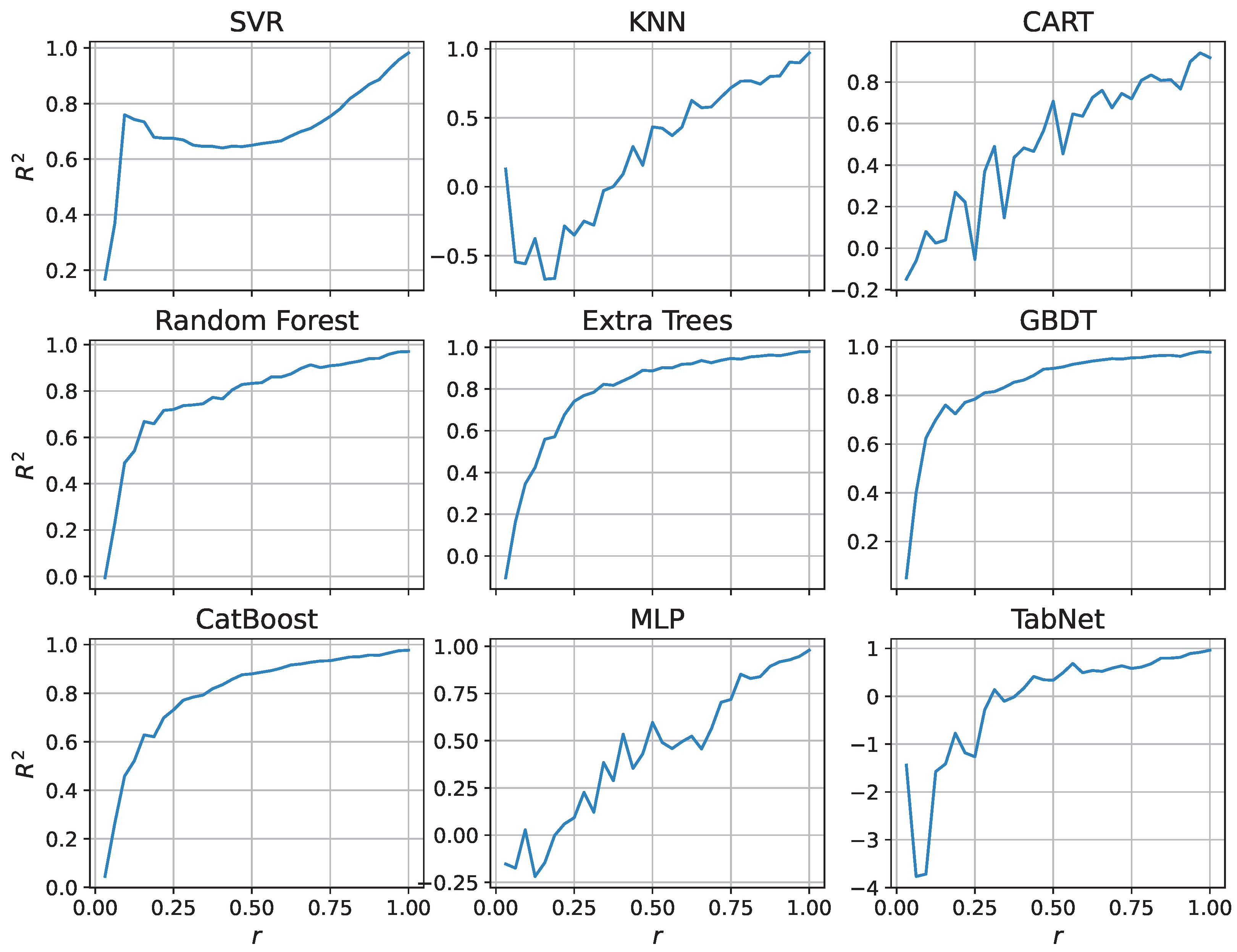
3.2. Model Robustness Under Feature Missingness

To evaluate model robustness, we simulated various levels of feature missingness using a uniform sampling strategy and assessed performance across different reservation ratios r. Each model was tested using its respective optimal hyperparameters from Figure 5. As shown in Figure 6, all the models exhibited improved performance (i.e., lower RMSE $E_r$) as the reservation ratio increased more values of features were retained during training and prediction.

Notably, single models demonstrated superior robustness compared with other approaches under conditions of high feature missingness. This advantage is attributed to the uniform sampling strategy, which helps maintain a relatively stable distance distribution, particularly benefiting models such as SVR and KNN.

Among the neural network models, TabNet required a really long time to train, yet its performance was not as remarkable as expected. As discussed in Section 2.4, this limitation stems from its feature selection mechanism, which lacks explicit attention to feature missingness. Specifically, it does not verify whether selected features are available or valid. However, this process does not incorporate any mechanism to identify or avoid missing features, meaning that missing values can still be selected and propagated.

In our experiments, we observed a result consistent with the analysis that the missing features were selected in the feature selection process. Furthermore, these missing values were then passed through the feature transformer and served as inputs to a shared fully connected layer. The underlying reason is the absence of an explicit mechanism for handling missing values within the attention mechanism.

As described in [33], the TabNet encoder applies an attentive transformer along with feature masking to select features at each decision step. The feature selection formula is given by $M\left[i\right]=sparsemax(P[i-1]·h_i\left(a[i-1]\right))$ where sparsemax encourages sparsity in the feature mask, and $P[i-1]={\prod }_{j=1}^i(\gamma -M\left[j\right])$ acts to suppress features already selected in previous steps. Here, $h_i\left(a[i-1]\right)$ is a trainable attentive transformer that guides feature selection for the current step.

Consequently, when critical features are missing, the model may be misled by incomplete or irrelevant information, leading to degraded performance. Introducing a more explicit indicator for missingness could help guide feature selection and mitigate the impact of misleading or unavailable features.

As shown in Figure 7, most models maintained relatively low variability with a coefficient of variation of $c_r<0.4$, indicating that K-fold cross-validation results were stable and reliable. Furthermore, the variability trends of tree-based models (except CART) were nearly identical: both RMSE and MAE first increased and then decreased with increasing r. Lastly, as depicted in Figure 8, $R^2$ scores suggest that regression results were more reliable when complete features were available. SVR achieved the highest $R^2$, highlighting its strong descriptive power in fully observed settings.

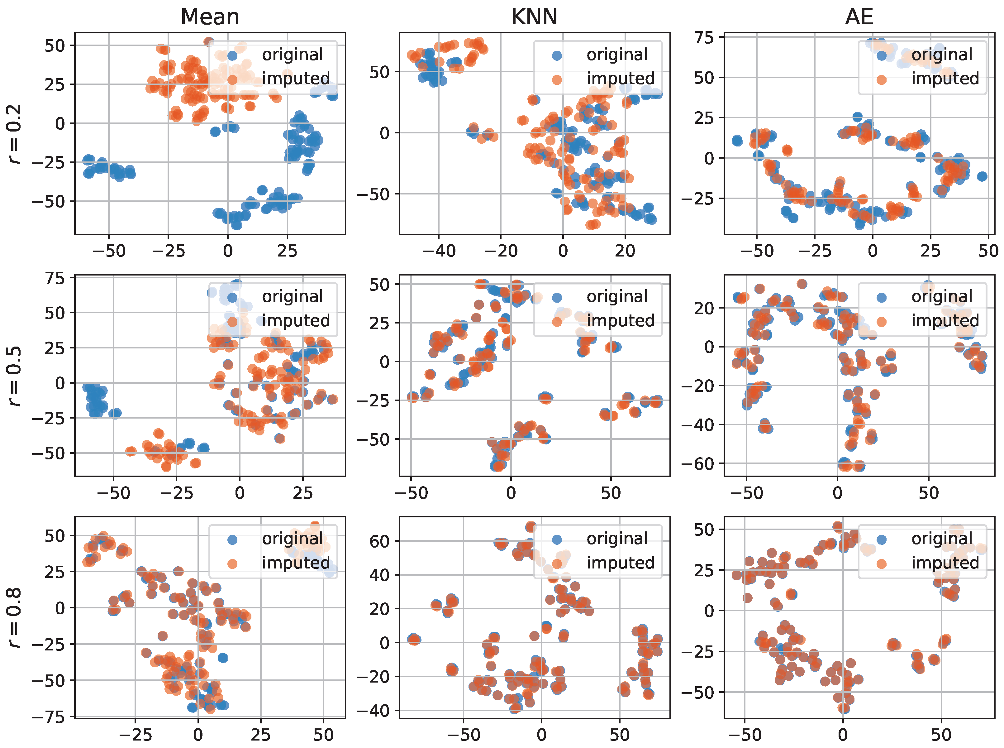
3.3. Imputation Evaluation

We applied the imputation and evaluation methods introduced in Section 2.3 to determine the most effective approach for addressing feature missingness.

For KNN imputation, the number of neighbors $n_e=1$ aligning with the optimal configuration of the KNN regression model obtained through hyperparameter tuning, as shown in Figure 5. The autoencoder was trained for 200 epochs, using the Adam optimizer, with a Cosine Annealing Learning Rate scheduler. The learning rate started at ${10}^{-2}$ and gradually decreased to ${10}^{-4}$. To improve generalization across different missing data distributions, we repeated the masking process 40 times with different random seeds, effectively expanding the training dataset.

To visually assess the quality of imputed features, we employed t-distributed Stochastic Neighbor Embedding (t-SNE) [44] to project the imputed feature spaces into two dimensions. This enabled a visual assessment of the data recovery quality by examining the degree of overlap between imputed and original data points. The t-SNE algorithm was configured with components of 2 for 2D visualization, perplexity of 5, learning rate of 50 for stable convergence, and a maximum of 1500 iterations to ensure sufficient optimization. The embedding was initialized randomly, and Euclidean distance was used to measure pairwise similarity.

During autoencoder training, the best mean NRMSEs obtained from validation were 0.06, 0.04, and 0.03 under varying levels of feature reservation. As shown in

Table 3. Imputation performance under different feature reservation ratios. The bold number indicates the best performance of each indicator.

Model	Feature Reservation Ratio r
	0.2	0.5	0.8
Mean imputation	0.23	0.17	0.11
KNN imputation	0.13	0.05	0.03
Autoencoder imputation	0.07	0.04	0.03

, the autoencoder generally outperformed both mean and KNN imputation methods, particularly under high missingness conditions. This advantage is further illustrated in Figure 9, where autoencoder reconstructions show closer alignment with the original data distribution.

However, as the feature reservation rate decreased, all three methods exhibited noticeable degradation in recovery quality, with evident divergence from the true feature distribution. These findings suggest that imputation is a viable approach when more than 50% of the features remain available, but its effectiveness diminishes under extreme missingness.

3.4. Mass Estimation

In real-world scenarios, fish are frequently partially occluded by other individuals or environmental elements, resulting in incomplete visibility. To simulate this condition more realistically, we considered two typical scenarios: occlusion caused by high-density groupings of fish and occlusion resulting from environmental shelters. For simplification, we defined two distinct visible regions: the head and the body, as illustrated in Figure 10. Specifically, the whole fish was segmented at the middle point of the dorsal fin; the region anterior to this point was defined as the head area, while the posterior region was defined as the body area.

As described in Section 2.1, we incorporated these visible regions into our sampling strategy. By retaining the observable points within these areas, we were able to expand the dataset outward from the visible zones, effectively increasing the diversity and realism of our samples.

Building on prior work, we evaluated our framework using autoencoder imputation combined with SVR (with hyperparameters optimized by grid search). For comparison, we also tested Extra Trees, a strong tree-based model, and MLP, a representative neural network approach. To enhance the training set, we repeated the region-based masking process 45 times using different random seeds.

As shown in

Table 4. Framework performance of various models on head and body areas. “Time” denotes the training duration. The bold number indicates the best performance of each indicator.

Model	Head				Body
	RMSE (g)	MAE (g)	${\mathit{R}}^{\mathbf{2}}$	Time (s)	RMSE (g)	MAE (g)	${\mathit{R}}^{\mathbf{2}}$	Time (s)
SVR [26]	21.10 ± 1.17	14.17 ± 0.50	0.98	1.68 ± 0.11	31.39 ± 1.75	21.66 ± 0.91	0.97	1.42 ± 0.07
Extra Trees [30]	2.49 ± 0.23	1.48 ± 0.11	1.00	0.08	4.47 ± 0.38	2.83 ± 0.24	1.00	0.09
MLP [20]	18.40 ± 1.24	13.10 ± 0.95	0.99	2.37 ± 0.65	25.21 ± 1.85	18.48 ± 1.47	0.98	3.07 ± 0.27
AE + SVR	6.53 ± 0.23	5.68 ± 0.07	1.00	1.66 ± 0.02	6.52 ± 0.32	5.67 ± 0.09	1.00	3.27 ± 0.03
AE + Extra Trees	1.95 ± 0.41	0.93 ± 0.16	1.00	1.49 ± 0.02	2.09 ± 0.45	1.01 ± 0.16	1.00	3.27 ± 0.09
AE + MLP	5.09 ± 1.90	3.27 ± 1.37	1.00	2.24 ± 0.11	3.99 ± 0.66	2.60 ± 0.41	1.00	4.39 ± 0.30

, our framework improved all evaluation metrics compared with the original data. For SVR, it achieved a 3.23-fold reduction (from 21.10 to 6.53 g) in the head area. We also observed that more visible features led to better results, with the head area performing best due to having more available features. Similarly, Extra Trees improved from 2.49 to 1.95 g, confirming the efficacy of our framework across model types. In terms of efficiency, these lightweight models trained in about 2 s, and the prediction time per sample was negligible. These results demonstrate the effectiveness of our method.

The overall process of our framework is visually depicted in Figure 10, which intuitively demonstrates how imputation restores structured missing features and supports subsequent regression.

4. Conclusions

To address the challenge of feature occlusion in computer vision-based fish biomass estimation using size-related features, we proposed a framework that combines feature imputation with regression modeling.

This study explores the relationship between size features and fish mass, aiming to facilitate the estimation of biomass from visual data. The methodology is generalizable and holds potential for application to other species. We systematically evaluated a variety of regression models, ranging from single models to tree-based methods and neural network architectures, with all the models optimized through grid search to ensure optimal performance.

To evaluate model performance and robustness under real-world conditions, we designed a feature missingness simulation strategy. Evaluation was conducted using cross-validation and multiple performance metrics, including RMSE, MAE, and $R^2$. Among all the models, SVR demonstrated the highest predictive accuracy, with an RMSE of 20.10, MAE of 13.75, and $R^2$ of 0.98. Tree-based models such as Extra Trees also performed competitively, reaching 21.92 in RMSE, 14.34 in MAE, and 0.98 in $R^2$. In contrast, TabNet showed instability, with RMSE fluctuating from 28.84 in 10-fold to 40.73 in 5-fold cross-validation.

Further, we evaluated multiple imputation strategies on an expanded dataset generated by 40-fold random masking. To measure imputation quality, we introduced mean NRMSE as a standardized evaluation metric. The results showed that autoencoder imputation consistently outperformed other methods, especially when the reservation ratio dropped below a threshold $r=0.2$, autoencoder imputation achieved RMSE improvements of approximately 2 times over KNN and 3 times over mean imputation. This highlights the importance of effective imputation in mitigating the impact of missing data.

In biomass estimation, we defined two types of visible regions: the head and the body. It was found that the head area, which contains more measurable features, exhibited better resilience to feature missingness. When applying our proposed framework, prediction accuracy improved significantly. For example, Extra Trees alone achieved an RMSE of 21.10, while the framework reduced it to 6.53 in the head area. This demonstrates that regions with more available features provide stronger robustness under occlusion.

On the basis of these findings, we propose a future research direction: the development of a hybrid regression framework that integrates feature complementation. This framework would infer missing features from existing ones and decouple the burden of missing data from the regression model itself. Such an approach holds promise for enhancing robustness in scenarios where occlusion or incomplete feature capture is common, particularly in computer vision applications.

This study primarily uses static images due to experimental and resource limitations, which currently prevent data collection in real production environments. While this may affect the applicability of our results, static images offer a controlled setting for preliminary validation and optimization. In future work, we plan to incorporate real-world data to further verify and enhance our framework.

References

1. Antonucci, F.; Costa, C. Precision aquaculture: A short review on engineering innovations. Aquac. Int. 2020, 28, 41–57. [Google Scholar] [CrossRef]
2. Føre, M.; Frank, K.; Norton, T.; Svendsen, E.; Alfredsen, J.A.; Dempster, T.; Eguiraun, H.; Watson, W.; Stahl, A.; Sunde, L.M.; et al. Precision fish farming: A new framework to improve production in aquaculture. Biosyst. Eng. 2018, 173, 176–193. [Google Scholar] [CrossRef]
3. Wu, Y.; Duan, Y.; Wei, Y.; An, D.; Liu, J. Application of intelligent and unmanned equipment in aquaculture: A review. Comput. Electron. Agric. 2022, 199, 107201. [Google Scholar] [CrossRef]
4. Davison, P.C.; Koslow, J.A.; Kloser, R.J. Acoustic biomass estimation of mesopelagic fish: Backscattering from individuals, populations, and communities. ICES J. Mar. Sci. 2015, 72, 1413–1424. [Google Scholar] [CrossRef]
5. Wanzenböck, J.; Mehner, T.; Schulz, M.; Gassner, H.; Winfield, I.J. Quality assurance of hydroacoustic surveys: The repeatability of fish-abundance and biomass estimates in lakes within and between hydroacoustic systems. ICES J. Mar. Sci. 2003, 60, 486–492. [Google Scholar] [CrossRef]
6. Takahara, T.; Minamoto, T.; Yamanaka, H.; Doi, H.; Kawabata, Z. Estimation of fish biomass using environmental DNA. PLoS ONE 2012, 7, e35868. [Google Scholar] [CrossRef]
7. Kamoroff, C.; Goldberg, C.S. Environmental DNA quantification in a spatial and temporal context: A case study examining the removal of brook trout from a high alpine basin. Limnology 2018, 19, 335–342. [Google Scholar] [CrossRef]
8. Zhang, J.; Chen, X.; Zhou, Q.; Diao, C.; Jia, H.; Xian, W.; Zhang, H. Species identification and biomass assessment of Gnathanodon speciosus based on environmental DNA technology. Ecol. Indic. 2024, 160, 111821. [Google Scholar] [CrossRef]
9. Abinaya, N.; Susan, D.; Sidharthan, R.K. Deep learning-based segmental analysis of fish for biomass estimation in an occulted environment. Comput. Electron. Agric. 2022, 197, 106985. [Google Scholar] [CrossRef]
10. Swethaa, S.; Sneha, E.; Sivasakthi, T. Fish biomass estimation based on object detection using YOLOv7. In Proceedings of the 2023 4th International Conference for Emerging Technology (INCET), Belgaum, India, 26–28 May 2023; pp. 1–6. [Google Scholar]
11. Tang, N.T.; Lim, K.G.; Yoong, H.P.; Ching, F.F.; Wang, T.; Teo, K.T.K. Non-intrusive biomass estimation in aquaculture using structure from motion within decision support systems. In Proceedings of the 2024 IEEE International Conference on Artificial Intelligence in Engineering and Technology (IICAIET), Kota Kinabalu, Malaysia, 26–28 August 2024; pp. 682–686. [Google Scholar]
12. Demer, D.A.; Hewitt, R.P. Bias in acoustic biomass estimates of Euphausia superba due to diel vertical migration. Deep. Sea Res. Part I Oceanogr. Res. Pap. 1995, 42, 455–475. [Google Scholar] [CrossRef]
13. Dejean, T.; Valentini, A.; Duparc, A.; Pellier-Cuit, S.; Pompanon, F.; Taberlet, P.; Miaud, C. Persistence of environmental DNA in freshwater ecosystems. PLoS ONE 2011, 6, e23398. [Google Scholar] [CrossRef] [PubMed]
14. Tsuji, S.; Ushio, M.; Sakurai, S.; Minamoto, T.; Yamanaka, H. Water temperature-dependent degradation of environmental DNA and its relation to bacterial abundance. PLoS ONE 2017, 12, e0176608. [Google Scholar] [CrossRef] [PubMed]
15. Saberioon, M.; Gholizadeh, A.; Cisar, P.; Pautsina, A.; Urban, J. Application of machine vision systems in aquaculture with emphasis on fish: State-of-the-art and key issues. Rev. Aquac. 2017, 9, 369–387. [Google Scholar] [CrossRef]
16. Li, D.; Hao, Y.; Duan, Y. Nonintrusive methods for biomass estimation in aquaculture with emphasis on fish: A review. Rev. Aquac. 2020, 12, 1390–1411. [Google Scholar] [CrossRef]
17. Fernandes, A.F.A.; de Almeida Silva, M.; de Alvarenga, E.R.; de Alencar Teixeira, E.; da Silva Junior, A.F.; de Oliveira Alves, G.F.; de Salles, S.C.M.; Manduca, L.G.; Turra, E.M. Morphometric traits as selection criteria for carcass yield and body weight in Nile tilapia (Oreochromis niloticus L.) at five ages. Aquaculture 2015, 446, 303–309. [Google Scholar] [CrossRef]
18. Zhang, T.; Yang, Y.; Liu, Y.; Liu, C.; Zhao, R.; Li, D.; Shi, C. Fully automatic system for fish biomass estimation based on deep neural network. Ecol. Inform. 2024, 79, 102399. [Google Scholar] [CrossRef]
19. Zhang, L.; Wang, J.; Duan, Q. Estimation for fish mass using image analysis and neural network. Comput. Electron. Agric. 2020, 173, 105439. [Google Scholar] [CrossRef]
20. Pedregosa, F.; Varoquaux, G.; Gramfort, A.; Michel, V.; Thirion, B.; Grisel, O.; Blondel, M.; Prettenhofer, P.; Weiss, R.; Dubourg, V. Scikit-learn: Machine learning in Python. J. Mach. Learn. Res. 2011, 12, 2825–2830. [Google Scholar]
21. Bishop, C.M.; Nasrabadi, N.M. Pattern Recognition and Machine Learning; Springer: Berlin/Heidelberg, Germany, 2006; Volume 4. [Google Scholar]
22. Deng, L.; Yu, D. Deep learning: Methods and applications. Found. Trends Signal Process. 2014, 7, 197–387. [Google Scholar] [CrossRef]
23. Marcelino, C.G.; Leite, G.M.; Celes, P.; Pedreira, C.E. Missing data analysis in regression. Appl. Artif. Intell. 2022, 36, 2032925. [Google Scholar] [CrossRef]
24. Tang, F.; Ishwaran, H. Random forest missing data algorithms. Stat. Anal. Data Min. Asa Data Sci. J. 2017, 10, 363–377. [Google Scholar] [CrossRef] [PubMed]
25. Ayilara, O.F.; Zhang, L.; Sajobi, T.T.; Sawatzky, R.; Bohm, E.; Lix, L.M. Impact of missing data on bias and precision when estimating change in patient-reported outcomes from a clinical registry. Health Qual. Life Outcomes 2019, 17, 1–9. [Google Scholar] [CrossRef] [PubMed]
26. Drucker, H.; Burges, C.J.; Kaufman, L.; Smola, A.; Vapnik, V. Support vector regression machines. Adv. Neural Inf. Process. Syst. 1997, 28, 779–784. [Google Scholar]
27. Muja, M.; Lowe, D.G. Fast approximate nearest neighbors with automatic algorithm configuration. VISAPP 2009, 2, 2. [Google Scholar]
28. Breiman, L.; Friedman, J.; Olshen, R.A.; Stone, C.J. Classification and Regression Trees; Routledge: London, UK, 2017. [Google Scholar]
29. Breiman, L. Random forests. Mach. Learn. 2001, 45, 5–32. [Google Scholar] [CrossRef]
30. Geurts, P.; Ernst, D.; Wehenkel, L. Extremely randomized trees. Mach. Learn. 2006, 63, 3–42. [Google Scholar] [CrossRef]
31. Friedman, J.H. Greedy function approximation: A gradient boosting machine. Ann. Stat. 2001, 29, 1189–1232. [Google Scholar] [CrossRef]
32. Dorogush, A.V.; Ershov, V.; Gulin, A. CatBoost: Gradient boosting with categorical features support. arXiv 2018, arXiv:1810.11363. [Google Scholar]
33. Arik, S.Ö.; Pfister, T. Tabnet: Attentive interpretable tabular learning. In Proceedings of the AAAI Conference on Artificial Intelligence, Virtual Event, 19–21 May 2021; Volume 35, pp. 6679–6687. [Google Scholar]
34. Gretton, A.; Borgwardt, K.M.; Rasch, M.J.; Schölkopf, B.; Smola, A. A kernel two-sample test. J. Mach. Learn. Res. 2012, 13, 723–773. [Google Scholar]
35. Thomas, T.; Rajabi, E. A systematic review of machine learning-based missing value imputation techniques. Data Technol. Appl. 2021, 55, 558–585. [Google Scholar] [CrossRef]
36. Batista, G.E.; Monard, M.C. A study of K-nearest neighbour as an imputation method. His 2002, 87, 48. [Google Scholar]
37. Jadhav, A.; Pramod, D.; Ramanathan, K. Comparison of performance of data imputation methods for numeric dataset. Appl. Artif. Intell. 2019, 33, 913–933. [Google Scholar] [CrossRef]
38. Duan, Y.; Lv, Y.; Kang, W.; Zhao, Y. A deep learning based approach for traffic data imputation. In Proceedings of the 17th International IEEE Conference on Intelligent Transportation Systems (ITSC), Qingdao, China, 8–11 October 2014; pp. 912–917. [Google Scholar]
39. Wong, L.Z.; Chen, H.; Lin, S.; Chen, D.C. Imputing missing values in sensor networks using sparse data representations. In Proceedings of the 17th ACM International Conference on Modeling, Analysis and Simulation of Wireless and Mobile Systems, Montreal, QC, Canada, 21–26 September 2014; pp. 227–230. [Google Scholar]
40. Breiman, L. Bagging predictors. Mach. Learn. 1996, 24, 123–140. [Google Scholar] [CrossRef]
41. Freund, Y.; Schapire, R.E. Experiments with a new boosting algorithm. In Proceedings of the ICML: Citeseer, Bari, Italy, 3–6 July 1996; Volume 96, pp. 148–156. [Google Scholar]
42. Sutton, C.D. Classification and regression trees, bagging, and boosting. Handb. Stat. 2005, 24, 303–329. [Google Scholar]
43. Mendes-Moreira, J.; Soares, C.; Jorge, A.M.; Sousa, J.F.D. Ensemble approaches for regression: A survey. ACM Comput. Surv. 2012, 45, 1–40. [Google Scholar] [CrossRef]
44. Van der Maaten, L.; Hinton, G. Visualizing data using t-SNE. J. Mach. Learn. Res. 2008, 9, 2579–2605. [Google Scholar]
Figure 1. The hyperparameter space spans multiple parameters across high-dimensional domains, making direct visualization challenging. To address this, we projected the space by calculating the Euclidean distance between each candidate configuration and the optimal one. This compression facilitates the intuitive interpretation of grid search trends and performance landscapes.
Fishes 10 00306 g001
Figure 2. Twelve traditional morphometric features (left), 1: total length, 2: standard length, 3: body height, 4: head height, 5: head length, 6: postorbital length, 7: torso length, 8: caudal peduncle length, 9: snout length, 10: eye diameter (not visualized), 11: interorbital width, 12: caudal peduncle depth. Eleven anatomical landmarks (right), 13: pectoral fin origin, 14: snout tip, 15: pelvic fin origin, 16: anterior margin of the scaled head area, 17: anal fin origin, 18: dorsal fin origin, 19: posterior end of the anal fin base, 20: posterior end of the dorsal fin base, 21: ventral origin of the caudal fin, 22: dorsal origin of the caudal fin, 23: base of the operculum. The 20 geometric morphometric features were derived from the 11 anatomical landmarks by calculating pairwise distances between selected points (e.g., the feature “13–14” represents the distance between landmarks 13 and 14).
Fishes 10 00306 g002
Figure 3. The Spearman correlation coefficients of all selected features indicate strong relevance to the target variable, ranging from 0.62 to as high as 0.99. Given this consistently high correlation, traditional morphometric and geometric morphometric features were combined into a unified feature set. This integration is justified by their collective contribution to model prediction performance.
Fishes 10 00306 g003
Figure 4. The architecture of the proposed autoencoder. The encoder transforms incomplete inputs into latent representations, and the decoder reconstructs the inputs to closely match the original data. Each hidden layer (FC) consists of a fully connected layer, followed by Batch Normalization and a ReLU activation.
Fishes 10 00306 g004
Figure 5. The results of the grid search for each model are presented, with all hyperparameter configurations detailed in Section 2.5. In each figure, the orange marker denotes the optimal hyperparameter combination, and the corresponding values are annotated in the lower-right corner of each subplot. For clarity, only configurations yielding a score below 150 were retained in the plots to reduce visual clutter and emphasize meaningful variations.
Fishes 10 00306 g005
Figure 6. The “mean” refers to the average RMSE across all folds at each reservation ratio r during 10-fold cross-validation. The “range” denotes the difference between the maximum and minimum RMSE values observed across the 10 folds, reflecting the variability in model performance.
Fishes 10 00306 g006
Figure 7. The coefficient of variation c r , computed for both RMSE and MAE across different reservation ratios r, quantifies the stability of model performance in 10-fold cross-validation.
Fishes 10 00306 g007
Figure 8. The mean R 2 values obtained from 10-fold cross-validation are presented, showing a general upward trend with increasing reservation ratios r. This trend complements the RMSE results presented in Figure 6, offering an additional view of model fit quality across varying levels of feature availability.
Fishes 10 00306 g008
Figure 9. Visualization of original and imputed feature distributions using t-SNE. “AE” denotes autoencoder. The original and imputed features (under different reservation ratios r and imputation methods) are projected into two dimensions for visual comparison. Note that t-SNE preserves relative distances, so axis values are not directly interpretable.
Fishes 10 00306 g009
Figure 10. Overview of the proposed framework. After feature extraction, imputation is performed before regression. The head area is located in the first rectangular region enclosed by the red dotted line, while the body area corresponds to the adjacent rectangular region on the right. Blue lines represent visible features from the head area, and green lines represent those from the body area.
Fishes 10 00306 g010