Climate Change and Freshwater Aquaculture: A Modified Slack-Based Measure DEA Approach

Abstract

As global climate change intensifies and resources become increasingly scarce, China’s sustainable development of freshwater aquaculture faces unprecedented challenges. This study utilizes panel data from 31 provincial-level regions in mainland China (2000–2023) and innovatively constructs a multi-stage sequential modified slack-based measure data envelopment analysis (MSBM-DEA) model. By endogenizing extreme climate factors within the aquaculture production efficiency framework, this study reveals the dynamic impact of climate change on freshwater aquaculture total factor productivity (TFP). The finding indicates that extreme climate events reduce freshwater aquaculture TFP by 1.66% and technical advancement by 18.9%. The impact varies regionally, with eastern provinces experiencing a maximum TFP decline of 3.1%, while western provinces face a significant drop of 5.2%. The eastern region, supported by technology and policy, shows a relatively strong recovery capacity, whereas the western region suffers more due to resource scarcity and technical lag. To tackle these challenges, this study recommends establishing a climate-adaptive TFP monitoring framework and promoting a dual-driven model of technical innovation and efficiency enhancement to bolster fisheries’ climate resilience. This research provides valuable decision making support for climate adaptation strategies in China’s freshwater aquaculture and serves as empirical evidence and theoretical guidance for other climate-vulnerable regions globally.

1. Introduction

As a crucial pillar of global food security, aquaculture contributes 46.8% of the total aquatic protein production worldwide and provides a primary source of livelihood for nearly 200 million people. Among these, freshwater aquaculture, with its resource adaptability and economic feasibility, accounts for 62.3% of the total global aquaculture production, becoming a key pathway for developing countries to achieve food security [1]. However, against the backdrop of intensifying climate change, this traditional production model is facing unprecedented risks. The Intergovernmental Panel on Climate Change of the United Nations (IPCC)’s Sixth Assessment Report (2023) points out that global freshwater ecosystems are under multiple pressures, including rising temperatures, increased frequency of extreme precipitation, and prolonged droughts. The combined effects of these climatic factors are surpassing the ecological and economic boundaries of freshwater aquaculture [2].

From a biological adaptation perspective, freshwater fish, as poikilotherms, exhibit significant nonlinear responses of metabolic rates and enzyme activities to water temperature [3]. When water temperatures exceed the tolerance threshold of specific species (for instance, the critical temperature for grass carp is 28 °C), it poses a risk of protein denaturation, which increases the probability of outbreaks of bacterial hemorrhagic septicemia by 3.2 times [4]. The pathological effects induced by thermal stress are transmitted through the food chain, ultimately leading to structural declines in the total factor productivity (TFP) of aquaculture systems. It is noteworthy that the impact of climate shocks on TFP exhibits heterogeneous transmission. Climatic factors not only affect the production front but also generate asymmetric transmission through dual channels of Technical Efficiency (TE) and Technical Progress (TP) [5]. Chinese freshwater aquaculture displays a dual characteristic of “high-density intensification” and “climate vulnerability.” Statistical data indicate that from 2000 to 2023, the total output of freshwater aquaculture in China grew at an average annual rate of 4.7%. However, the climate elasticity coefficient of unit output decreased from 0.18 to −0.12 [6], indicating that the marginal effect of climate change has shifted from a positive promotion to a negative suppression.

The existing literature has employed Solow Residual Method and Data Envelopment Analysis (DEA) and its derivative models, such as the Malmquist Index, to quantify fluctuations in total factor productivity (TFP) [7,8]. While the Solow Residual Method is widely utilized, it fails to adequately consider the impact of technical progress. Conversely, Production Function methods may become ineffective in complex ecological systems due to their inherent assumptions. Traditional DEA methods have the advantage of measuring the efficiency of multi-input and multi-output systems, as well as analyzing dynamic changes and the sources of productivity. However, traditional DEA methods do not capture the implication of extreme weather as negative inputs on TFP. Therefore, we utilize MSBM-DEA to identify it.

Notably, Letta M initiated an exploration of the impacts of exogenous variables, including climate change, on TFP. These exogenous factors, such as rising water temperatures and water resource scarcity, have been shown to significantly influence the efficiency of aquaculture production and the sustainable utilization of resources [9]. However, several gaps persist in the modeling of climate–economy coupling systems: First, conventional models often consider climate variables as exogenous shocks, neglecting the endogenous interaction effects between climate factors and production inputs like capital and labor. Second, the nonlinear impact mechanisms of climate factors remain poorly understood, particularly concerning the threshold effects of extreme climate events on TFP. Third, while global research has predominantly focused on marine fisheries, there exists a notable paucity of studies examining freshwater aquaculture.

In response to the theoretical limitations and practical needs, this study constructs a climate-adaptive total factor productivity analysis framework. The methodological innovations encompass three aspects: Firstly, we introduce the Mixed Slack-Based Model (MSBM-DEA) proposed by Sharp et al. [10], which incorporates a Sequential Correction Mechanism to address the sensitivity bias of traditional DEA models to climate shocks. Secondly, we develop a Disaster Impact Index (DII) to quantify the composite effects of extreme high temperatures, extreme low temperatures, extreme precipitation, and extreme drought. Finally, we apply dynamic panel data decomposition techniques to reveal the transmission pathways through which climate factors affect TFP via Technical Efficiency channels. The study uses balanced panel data from 31 provincial-level administrative regions in China from 2000 to 2023 to systematically assess the intensity and mechanisms of climate change’s impact on the TFP of Chinese freshwater aquaculture.

The findings not only provide micro-level evidence for developing countries to formulate climate-resilient fisheries policies but also expand the analytical paradigm of fisheries economics in non-stationary environments. By integrating a climate-adaptive total factor productivity (TFP) monitoring framework with a dual-driven model of technical innovation and efficiency improvement, this research emphasizes the crucial role of adaptive strategies in bolstering fisheries’ capacity to mitigate climate change impacts. This innovative approach enables a comprehensive assessment of how fisheries can optimize productivity under changing climate conditions while addressing complex environmental challenges.

Furthermore, the insights derived from this study extend beyond the field of fisheries economics and offer valuable perspectives for industries facing similar environmental issues. By adopting an interdisciplinary approach, we aim to foster dialog and collaboration across different sectors, strengthening the collective capacity to address the complex impacts of climate change. Therefore, the methodologies and findings presented in this paper aim to resonate with a broader range of stakeholders, enhancing their ability to devise effective strategies in the face of global climate challenges.

2. Materials and Methods

Within the output dimension, a dual perspective is adopted for the evaluation framework. On the expected output side, key indicators include the total output value of freshwater aquaculture and the production volume of freshwater fish. The former reflects the economic contribution of outputs, while the latter indicates the physical scale of production. Together, these indicators establish a dual verification mechanism for assessing economic benefits. In contrast, the undesirable output side incorporates carbon emissions from freshwater aquaculture.

The carbon emissions from freshwater aquaculture mainly come from two aspects: direct carbon emissions and indirect carbon emissions. Firstly, direct carbon emissions originate from energy combustion. This paper characterizes the carbon emissions produced by freshwater aquaculture fishing vessels burning diesel. During the freshwater aquaculture process, fishing vessels perform several key tasks that are crucial for aquaculture efficiency and sustainable development. Specifically, these vessels are responsible for the transportation and distribution of feed, the capture of fry and mature fish, facility maintenance, and water quality monitoring in cage and pen aquaculture. Furthermore, although the small, motorized fishing boats used in most pond aquaculture differ in type from the vessels used in cage aquaculture, they also play an irreplaceable role in tasks such as capture, water quality monitoring, and facility maintenance. Secondly, indirect carbon emissions result from the use of electricity. Most freshwater aquaculture methods primarily rely on natural resources such as water and land, leading to a relatively low dependence on energy. However, pond aquaculture and intensive farming exhibit a higher energy dependence, particularly referring to the indirect carbon emissions generated from oxygen supply and electricity consumption during the processes of pond and intensive aquaculture. The specific formula for calculating carbon emissions is articulated as follows [11]:

$$C=Pa{\theta }_1\gamma +\left(Q\beta +S\eta \right){\theta }_2\gamma$$

(1)

where $C$ represents the total carbon emissions from freshwater aquaculture and $P$ denotes the total power of fishing vessels. Since freshwater fishing is relatively limited, we derived the fuel consumption for freshwater fisheries based on the proportion of outputs from freshwater and seawater fisheries. $\alpha$ is the fuel consumption coefficient for the vessels, determined to be 0.225 tons/kilowatt according to the “Reference Standards for Calculating Oil Consumption for Subsidies to Domestic Motor Fishing Vessels [12]”. $Q$ and $S$ represent the production volumes for freshwater pond aquaculture and intensive aquaculture, respectively. $\beta$ and $\eta$ are the electricity consumption coefficients per unit of production for pond and intensive aquaculture, with values of 0.37 kilowatt-hours/kilogram and 8.66 kilowatt-hours/kilogram, respectively. The coefficients ${\theta }_1$ and ${\theta }_2$ denote the energy conversion factors for diesel and electricity, which are established based on the “China Energy Statistical Yearbook”, with values of 1.4571 kg of standard coal per kilogram and 0.1229 kg of standard coal per kilowatt-hour, respectively. $\gamma$ is the carbon emission coefficient, valued at 2.493 kg per kilogram of standard coal [13]. This model employs the Life Cycle Assessment (LCA) methodological framework to achieve estimates of carbon emissions across the entire aquaculture system.

The construction of the production factor input system follows the theory of production functions, selecting labor, land, and capital as the core input variable [14]. Labor input is represented by the number of employed persons, while land input is measured by the area of freshwater aquaculture water bodies. Capital input is decomposed into two components: fixed assets (total power of fishing vessels) and variable inputs (such as seedlings and feed). Notably, the input of seedlings is represented by the stocking quantity of fish fry (in hundreds of millions), which avoids the measurement errors associated with live biological metrics and aligns with the cyclical characteristics of freshwater aquaculture production. Building on this foundation, an innovative approach is taken by introducing the Regional Dynamic Fisheries Disaster Impact Index (DII) as a proxy variable for climate shocks, thereby challenging the exogeneity assumption of climate factors in traditional productivity measurement models. Compared with conventional assessment systems, this model quantifies the dynamic impact of climate change on production boundaries by integrating the DII into the production function, thus better reflecting the non-stationary characteristics of aquaculture production while keeping the output variables constant.

Table 1. Key indicators of freshwater aquaculture production input and output.

Indicator	Indicator Category	Variable	Variable Description		Unit
Input		Traditional Inputs	Labor Force	Number of professionals engaged in freshwater aquaculture	Persons
			Cultivation Area	Total area of freshwater aquaculture	Hectares
			Seedlings	Number of freshwater fish seedlings	10,000
			Fixed Assets	Total power of freshwater aquaculture machinery vessels	Kilowatts
		Climate Factors	DII	Regional dynamic freshwater aquaculture disaster impact index	-
Output		Economic Growth	Economic Output	Total output value of freshwater aquaculture	10,000 CNY
			Economic Output	Total production of freshwater aquaculture	Tons
Environmental Impact		Environmental Impact	Carbon Emissions	Carbon emissions from freshwater aquaculture operations	Tons

Note: DII = Disaster Impact Index.

and

Table 2. Descriptive statistics of input and output factors in freshwater aquaculture.

Indicator (Freshwater Aquaculture)	Observations	Unit	Mean Value	Standard Deviation	Minimum Value	Maximum Value
Number of People Employed	744	Persons	243,070.74	283,436.87	19.00	1,402,644.00
Total Area	744	Hectares	165,975.84	176,910.49	2.00	886,963.00
Number of Seedlings	744	100,000	323.90	1181.86	0.00	8633.00
Total Power of Machinery	744	Kilowatts	19,426.2	50,613.09	0.00	1,217,331.00
DII	744	-	−43.89	8.73	−84.34	−19.08
Total Output Value	744	CNY 100 Million	1,558,474.0	2,630,481.00	227.20	32,200,000.00
Total Production	744	Tons	792,215.40	1,020,396.00	3.03	5,206,376.00
Carbon Emissions	744	Tons	556,860.90	890,005.30	3.74	4,053,253.00

Note: DII = Disaster Impact Index.

show the following content.

The output indicators exhibit a pronounced right-skewed distribution, with the total production value ranging from 227.2 million CNY to 3.2 billion CNY, while the physical output varies from 303,000 tons to 5,210,000 tons, with a mean of 792,215.40 tons and a standard deviation of 1,020,396 tons. Carbon emissions demonstrate the highest variability, with an average of 556,860.90 tons, a standard deviation of 890,005.30 tons, and a coefficient of variation reaching 159.9%, indicating significant differences in environmental impacts across different production systems. The Regional Disaster Impact Index is quantified using a standardized dimensionless metric, with a mean of −43.89 (indicating negative inputs) and a standard deviation of 8.73, while the extreme values range from −84.34 to −19.08, reflecting variability in climate vulnerability. Notably, the coefficient of variation for all inputs and outputs exceeds 100%, indicating substantial scale differences; thus, logarithmic transformation of the data is necessary prior to conducting efficiency analysis.

2.1. Construction and Validation of the Regional Dynamic Fisheries Disaster Impact Index (DII)

Standardization of Extreme Climate Indicators

Considering that extreme climate indicators primarily encompass extreme low temperatures, high temperatures, precipitation, and droughts, a standardized approach is employed to construct a unified climate risk index that accounts for the inherent differences among these extreme climate indicators. Following Guo et al.’s methodology proposed, the original data undergo extreme value standardization [15]. Taking the number of extreme low temperature days (LTD) as an illustrative example, the standardization formula can be expressed as follows:

$$\overline{LT{D}_{m,n}}={\displaystyle \frac{LT{D}_{m,n}-\underset{k=1,\dots ,K;l=1,\dots ,L}{\min }\left(LT{D}_{k,l}\right)}{\underset{k=1,\dots ,K;l=1,\dots ,L}{\max }\left(LT{D}_{k,l}\right)-\underset{k=1,\dots ,K;l=1,\dots ,L}{\min }\left(LT{D}_{k,l}\right)}}\times 100$$

(2)

During data integration, the total number of countries and the total number of sample years are incorporated into the analytical framework. Using this methodology, sub-indices for extreme low temperature days (LTD), extreme high temperature days (HTD), extreme rainfall days (ERD), and extreme drought days (EDD) are calculated. Subsequently, a dynamic weighting coefficient method is employed, utilizing these four sub-indices as the foundational elements for constructing the freshwater aquaculture disaster index for the 31 provinces of China.

Given the spatial heterogeneity in seasonal patterns and climate impacts, particularly the differential weight of each climate factor’s impact on disasters, it is imperative to implement a dynamic weighting distribution for these four indicators. This establishes the Regional Dynamic Fisheries Disaster Impact Index (DII), which aims to comprehensively assess the impact of climatic events on fisheries’ activities across different regions and provide a theoretical foundation for the formulation of relevant policies:

$$\mathrm{D}\mathrm{I}{\mathrm{I}}_{\mathrm{m},\mathrm{n}} = {\mathsf{\omega }}_1 \overline{\mathrm{L}\mathrm{T}{\mathrm{D}}_{\mathrm{m},\mathrm{n}}} + {\mathsf{\omega }}_2 \overline{\mathrm{H}\mathrm{T}{\mathrm{D}}_{\mathrm{m},\mathrm{n}}} + {\mathsf{\omega }}_3 \overline{\mathrm{E}\mathrm{R}{\mathrm{D}}_{\mathrm{m},\mathrm{n}}} + {\mathsf{\omega }}_4 \overline{\mathrm{E}\mathrm{D}{\mathrm{D}}_{\mathrm{m},\mathrm{n}}}$$

(3)

We chose the time series from 2000 to 2023 due to the availability of comprehensive extreme climate data in Guo et al. [15] and the reliability of data from the China Fishery Yearbook for this period. Based on the classification of geographic and economic characteristics by the National Bureau of Statistics of China, this study divides the 31 provinces of mainland China into 3 climatic regions: the Eastern Region (11 provinces: Beijing, Tianjin, Hebei, Liaoning, Shanghai, Jiangsu, Zhejiang, Fujian, Shandong, Guangdong, and Hainan); the Central Region (8 provinces: Shanxi, Jilin, Heilongjiang, Anhui, Jiangxi, Henan, Hubei, and Hunan); and the Western Region (12 provinces: Inner Mongolia, Guangxi, Chongqing, Sichuan, Guizhou, Yunnan, Tibet, Shaanxi, Gansu, Qinghai, Ningxia, and Xinjiang).

2.2. Dynamic Weight Allocation Strategy

To quantify the impact of climate disasters on freshwater fisheries’ Total Factor Productivity (TFP), this study designs a dual allocation scheme to verify the robustness of weight distribution:

2.2.1. Baseline Equal Weighting

This scheme follows the benchmark framework for climate disaster assessment proposed by Kun Guo [15] and incorporates the national standard “Meteorological Drought Classification” (GB/T 20481-2017) [16]. The principle of equal weight allocation is adopted and assigned a weight of 0.25 to each indicator. The baseline method aligns with the internationally accepted “Equal Weighting without Priori” criterion [17], whose theoretical foundation lies in the premise that, in cases of uncertainty regarding the contribution of multiple indicators, equal weighting can effectively mitigate subjective bias while adhering to the principle of minimum information loss [18]. This approach has been validated by 30 global studies on climate risk assessment, demonstrating significant methodological generalizability.

Under this scheme, the weights are uniformly set at 0.25 for each indicator based on the equal weighting principle, drawing from Kun Guo’s proposed climate disaster assessment benchmark framework. This weighting strategy also conforms to the guidance provided in Appendix C of “Meteorological Drought Classification” [15], which states: “In the absence of prior knowledge regarding the contribution of multiple indicators, equal weighting should be adopted as a baseline reference scheme.”

2.2.2. Symmetric Perturbation Weights

To systematically evaluate the sensitivity of weight allocation, the “Symmetric Perturbation Method” recommended by the IPCC [19] is employed to construct 12 perturbation experimental schemes (4 for each of the Eastern, Central, And Western Regions). The specific implementation steps include:

Positive perturbation: The weight of LTD (extreme low temperature days) is adjusted to 0.275 (an increase of 10%), while the weights of other indicators are correspondingly adjusted to 0.242 (a decrease of 3.2%), simulating a disaster scenario dominated by extreme low temperatures.

Negative perturbation: The weight of LTD is reduced to 0.225 (a decrease of 10%), while the weights of other indicators are increased to 0.258 (an increase of 3.2%), evaluating the impact of weakened LTD weight on the composite index.

Cross-dimensional perturbation: Similar operations are applied sequentially to HTD (extreme high temperature days), ERD (extreme rainfall days), and EDD (extreme drought days), forming the following data table. (As shown in Appendix A,

Table A1. Symmetric disturbance weight schemes of Disaster Impact Indicator for Eastern, Central, and Western Regions of China.

Region	Weight Scheme	Indicator Weight	$\mathbf{Spearman}’\mathbf{s} \mathit{\rho }$
Eastern	Positive (Negative) Disturbance of LTD	0.275, 0.242, 0.242, 0.242 (0.225, 0.258, 0.258, 0.258)	0.9989
	Positive (Negative) Disturbance of HTD	0.242, 0.275, 0.242, 0.242 (0.258, 0.225, 0.258, 0.258)	0.9887
	Positive (Negative) Disturbance of ERD	(0.242, 0.242, 0.275, 0.242) (0.258, 0.258, 0.225, 0.258)	0.9892
	Positive (Negative) Disturbance of EDD	0.242, 0.242, 0.242, 0.275 (0.258, 0.258, 0.258, 0.225)	0.9576
Western	Positive (Negative) Disturbance of LTD	0.275, 0.242, 0.242, 0.242 (0.225, 0.258, 0.258, 0.258)	0.9884
	Positive (Negative) Disturbance of HTD	0.242, 0.275, 0.242, 0.242 (0.258, 0.225, 0.258, 0.258)	0.9395
	Positive (Negative) Disturbance of ERD	0.242, 0.242, 0.275, 0.242 (0.258, 0.258, 0.225, 0.258)	0.9879
	Positive (Negative) Disturbance of EDD	0.242, 0.242, 0.242, 0.275 (0.258, 0.258, 0.258, 0.225)	0.9881
Central	Positive (Negative) Disturbance of LTD	0.275, 0.242, 0.242, 0.242 (0.225, 0.258, 0.258, 0.258)	0.9398
	Positive (Negative) Disturbance of HTD	0.242, 0.275, 0.242, 0.242 (0.258, 0.225, 0.258, 0.258)	0.9873
	Positive (Negative) Disturbance of ERD	0.242, 0.242, 0.275, 0.242 (0.258, 0.258, 0.225, 0.258)	0.9589
	Positive (Negative) Disturbance of EDD	0.242, 0.242, 0.242, 0.275 (0.258, 0.258, 0.258, 0.225)	0.9891

presents the symmetric disturbance weight schemes of disaster impact indicators for Eastern, Central, and Western Regions of China).

After determining the 12 perturbation schemes, stability tests were conducted. Spearman’s coefficient, as a non-parametric method, is particularly well suited to ecological datasets due to its ability to handle non-normal distributions and outliers, while effectively capturing rank-based associations to evaluate relative changes between variables. A sensitivity analysis based on Spearman’s rank correlation coefficient was employed to systematically test the weight parameters, with a two-tailed significance level set at α = 0.01 [19,20].

First, we calculated the rank correlation ($\rho$) between the original ranking and the disturbed ranking to quantify the impact of weight adjustments on ranking consistency. Second, a permutation test was conducted to generate a null distribution, and the two-tailed significance level (α = 0.01) was used to verify the statistical significance of $\rho$. Using this process, we calculated Spearman’s rank correlation coefficient. The test results indicate that, across the 12 perturbation schemes, the mean Spearman correlation coefficient for regional disaster risk rankings is 0.927, with a maximum value of 0.963 (Eastern Region) and a minimum value of 0.891 (Western Region). According to the statistical critical value table [21], when $\rho$ ≥ 0.8, the method can be considered to exhibit strong robustness. This indicates that the DII has strong weight robustness. Therefore, the baseline weight will be maintained, and the weight will be uniformly set to 0.25.

2.3. Incorporation of Climate Factors in the Total Factor Productivity (TFP) Analysis Framework for Freshwater Aquaculture

2.3.1. Selection of the Base Model and Endogenous Integration of Climate Variables

This study employs the Dynamic Data Envelopment Analysis (DEA) method to calculate the Total Factor Productivity (TFP) of fisheries across 31 provinces (municipalities) in China from 2000 to 2023, along with the dynamic changes in its decomposition. In this framework, it is assumed that the $\mathrm{j}\left(\mathrm{j}=\mathrm{1,2},\dots ,\mathrm{J}\right),$ Production Unit $\left(\mathrm{P}\mathrm{U}\right)\mathrm{a}\mathrm{t}\mathsf{\tau }\mathrm{t}\mathrm{h}\left(\mathsf{\tau }=\mathrm{1,2},\dots ,\mathrm{T}\right)$, time point utilizes $\mathrm{p}\left(\mathrm{p}=\mathrm{1,2},\dots ,\mathrm{P}\right)$, types of input resources $a_{j,p}^{\mathsf{\tau }}$ to produce $\mathrm{q}(\mathrm{q}=1,2,\dots ,\mathrm{Q})$ types of outputs $b_{j,p}^{\mathsf{\tau }}$. The $\mathrm{P}$ types of inputs include traditional factors such as freshwater fisheries area and fry stock, as well as climate parameters. Referring to the dynamic frontier technology proposed by Shestalova, the intertemporal reference technology under Variable Returns to Scale (VRS) is defined as follows [22]:

$${\mathcal{F}}^{\mathsf{\tau }}\left(a^{\mathsf{\tau }}\right)=\{b:b_{j,q}^{\mathsf{\Gamma }}\le \sum _{\mathsf{\iota }=1}^{\mathsf{\Gamma }}\sum _{j=1}^J{\mathsf{\omega }}_j^{\mathsf{\tau }}{b}_{j,q}^{\mathsf{\iota }},\hspace{0.25em}\forall q;a_{j,p}^{\mathsf{\Gamma }}\ge \sum _{\mathsf{\iota }=1}^{\mathsf{\Gamma }}\sum _{j=1}^J{\mathsf{\omega }}_j^{\mathsf{\tau }}{a}_{j,p}^{\mathsf{\iota }},\hspace{0.25em}\forall p;\sum _{\mathsf{\iota }=1}^{\mathsf{\Gamma }}\sum _{j=1}^J{\mathsf{\omega }}_j^{\mathsf{\tau }}=1,\hspace{0.25em}{\mathsf{\omega }}_j^{\mathsf{\tau }}\ge 0,\hspace{0.25em}\forall j\}.$$

(4)

where $\mathsf{\tau }$ is the time point index; $a^{\tau }\mathrm{a}\mathrm{n}\mathrm{d} b^{\tau }$ represent the input and output vectors for all PUs; and ${\omega }^{\tau }$ represents the weight coefficients at time $\tau$.

2.3.2. Dynamic Frontier Correction Mechanism

In constructing the efficiency evaluation model, this study adopts the Slacks-Based Measure (SBM) proposed by Tone [23]. The SBM model evaluates the inefficiency of a decision-making unit (DMU) by incorporating input and output slack variables. Its objective function is given by:

$$\min \mathsf{\eta }={\displaystyle \frac{1-\frac{1}{P}{\sum }_{p=1}^P\left(\frac{{\mathsf{\delta }}_p^{-}}{R_{p,j}}\right)}{1+\frac{1}{Q}{\sum }_{q=1}^Q\left(\frac{{\mathsf{\delta }}_q^{+}}{R_{q,j}}\right)}}$$

(5)

subject to the constraints

$$\begin{gathered} A\mu +, {\delta }^{-}=a_j \\ B\mu -{\delta }^{+}=b_j \\ \mathsf{\Sigma }\mu =1 \\ \mu ,{\delta }^{+}, {\delta }^{-}\ge 0 \end{gathered}$$

(6)

$R_{p,j}=a_{p,j}-\underset{j}{\min }\left(a_j\right), R_{q,j}=\underset{j}{\max }\left(b_j\right)-b_{q,j},$ where $\mathsf{\eta }$ represents the normalized efficiency value, ${\delta }_p^{-}$ denotes the redundancy of input type p, ${\delta }_q^{+}$ represents the gap in output type q, and $\mu$ is the weight vector. $A\mu$ and $B\mu$ represent the input and output levels below the frontier surface, respectively.

The SBM model does not require the specification of weights, and the resulting efficiency score ranges between 0 and 1, making it easy to interpret. To address the issue of negative inputs caused by climate factors, Sharp et al. proposed the Modified Slacks-Based Measure (MSBM) based on Tone’s original formulation [10]. First, it applies standardized ranges for inputs and outputs to normalize slack variables, ensuring that efficiency scores remain non-negative. Second, it introduces adjustable input and output weights that are normalized, enhancing the model’s adaptability to diverse data characteristics. Third, the model attains translation invariance, allowing it to handle datasets with negative values or those affected by linear shifts.

2.4. Dynamic Decomposition of TFP Under Climate Constraints

Reconstruction of the Malmquist Index

Based on the methods proposed by Caves et al., the dynamic Malmquist productivity index is constructed as follows [15]:

$$\begin{gathered} \mathcal{H}\left(a^{\mathsf{\tau }+1},b^{\mathsf{\tau }+1},a^{\mathsf{\tau }},b^{\mathsf{\tau }}\right)={\left[\left({\displaystyle \frac{D^{\mathsf{\tau }}\left(a^{\mathsf{\tau }+1},b^{\mathsf{\tau }+1}\right)}{D^{\mathsf{\tau }}\left(a^{\mathsf{\tau }},b^{\mathsf{\tau }}\right)}}\right)\times \left({\displaystyle \frac{D^{\mathsf{\tau }+1}\left(a^{\mathsf{\tau }+1},b^{\mathsf{\tau }+1}\right)}{D^{\mathsf{\tau }+1}\left(a^{\mathsf{\tau }},b^{\mathsf{\tau }}\right)}}\right)\right]}^{1/2} \\ \begin{array}{c}={\displaystyle \frac{D^{\mathsf{\tau }+1}\left(a^{\mathsf{\tau }+1},b^{\mathsf{\tau }+1}\right)}{D^{\mathsf{\tau }}\left(a^{\mathsf{\tau }},b^{\mathsf{\tau }}\right)}}\times {\left[{\displaystyle \frac{D^{\mathsf{\tau }}\left(a^{\mathsf{\tau }+1},b^{\mathsf{\tau }+1}\right)}{D^{\mathsf{\tau }+1}\left(a^{\mathsf{\tau }+1},b^{\mathsf{\tau }+1}\right)}}\times {\displaystyle \frac{D^{\mathsf{\tau }}\left(a^{\mathsf{\tau }},b^{\mathsf{\tau }}\right)}{D^{\mathsf{\tau }+1}\left(a^{\mathsf{\tau }},b^{\mathsf{\tau }}\right)}}\right]}^{1/2}\\ =TE\times TP\end{array} \end{gathered}$$

(7)

In this context, the “Technical Efficiency (TE)” reflects the extent to which production units (PUs) in each province can catch up with the best-performing producers over the period from t to t + 1. Specifically, the index quantifies the degree of convergence of these provinces toward the optimal production frontier during this time frame. A higher TEC indicates a greater improvement in efficiency as provinces adopt best practices and technologies from the leading producers. The “Technical Progress (TP) index” denotes the movement of the technology frontier itself between time periods t and t + 1. This index reflects advancements in technology that enhance production capabilities and improve the overall efficiency of resources. As the technology frontier shifts outward, it sets a new benchmark for productivity, which all production units must strive to achieve.

This study incorporates climate factors into the input system and employs the dynamic MSBM-DEA model for a comprehensive analysis, thereby providing an in-depth interpretation of the spatiotemporal differential characteristics of China’s freshwater aquaculture TFP under the influence of climate constraints.

3. Results

3.1. DII Regional Disparity Results

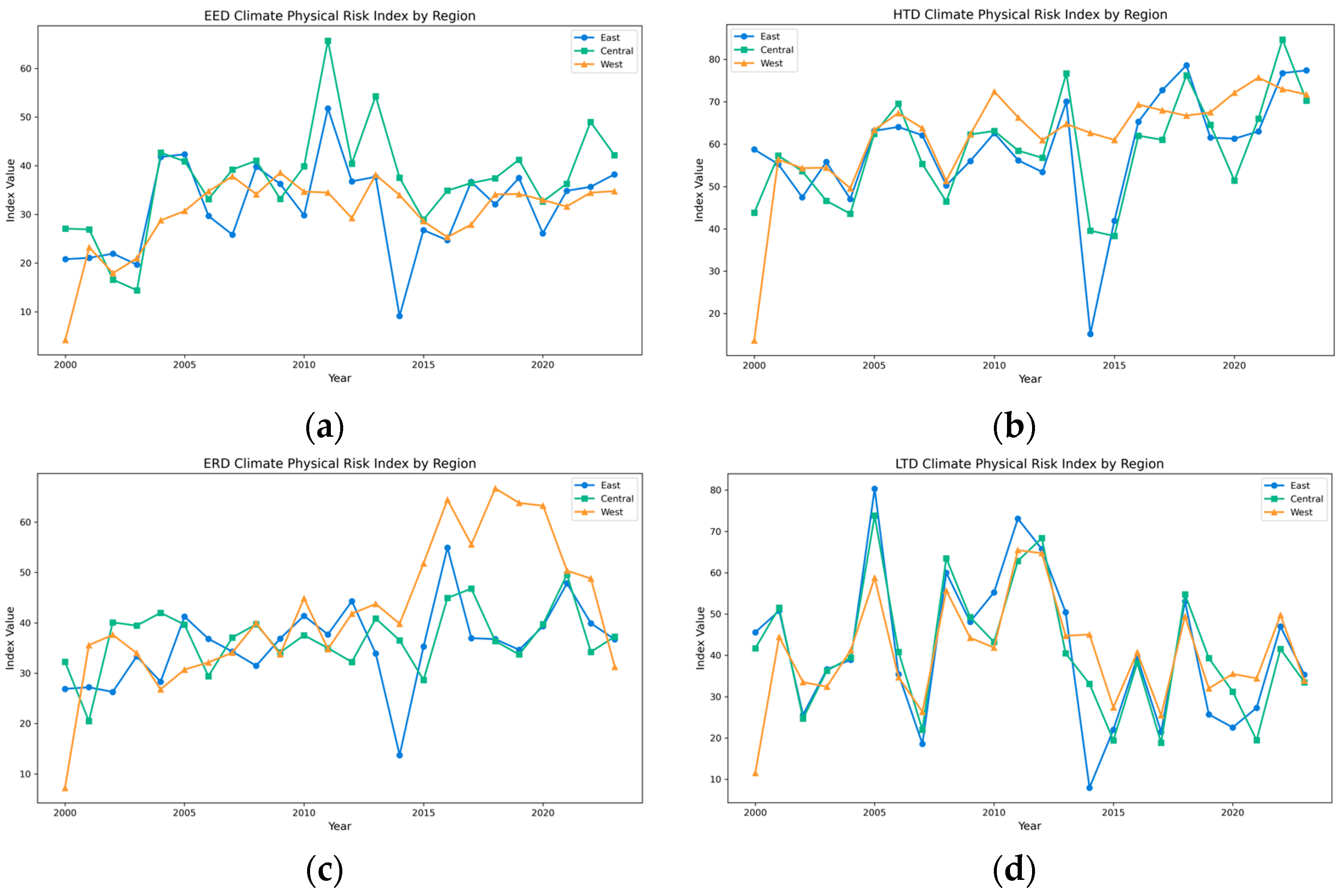
As illustrated, extreme climate events in China exhibit significant spatial disparities from the Eastern to the Western Regions. Figure 1 shows the average annual growth rates of extreme high temperature days (HTD) and extreme drought days (EDD) in the Western Region are 6.8% and 5.3%, respectively, demonstrating an exponential growth trend, which is 5–6 times the rates observed in the Eastern Region. In the context of climate warming, the rate of evaporation in the western arid regions significantly exceeds the increase in precipitation, exacerbating the frequency of extreme drought events (EDD) and further intensifying the persistence of extreme high temperatures (HTD). As a transitional zone for climate impacts, the Central Region reflects varying adaptability and vulnerability to climate change across the different areas. Notably, extreme climate events nationwide exhibit a synchronous diffusion characteristic; in 2022, the number of extreme high temperature days (HTD) in the Eastern, Central, and Western regions all surpassed 70 days, representing a 29.3% increase from the year 2000. Furthermore, the difference in HTD between the Eastern and Western regions decreased from 45.07 days in 2000 to 5.67 days in 2023, indicating that high-temperature events are spreading from localized hotspots to a more widespread phenomenon.

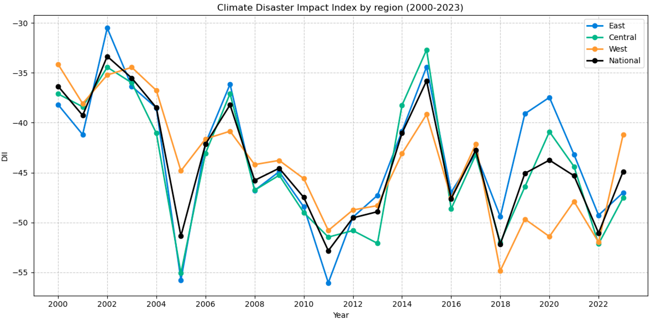
Figure 2 illustrates the evolution of the Climate Disaster Impact Index (DII) for mainland China’s Eastern, Central, and Western regions, as well as the national average, from 2000 to 2023, using line charts. Three main trends are observed: First, the DII values in all regions show an upward trend (ranging from 30 to 55), indicating a persistent increase in climate stress faced by freshwater fisheries systems. The national average (black solid line) rose from 38.2 in 2000 to 51.6 in 2023, representing a 35.1% increase. Second, there are significant regional disparities, with the DII in the Eastern Region consistently being the highest (peaking at 54.3 in 2022), followed by the Central Region (50.1 in 2023) and the Western Region (47.8 in 2023). This disparity may be related to spatial variations in risks associated with coastal storms in the East, flooding in the Central Region, and droughts in the West. Third, the DII growth rate notably accelerated after 2015 (averaging +1.32 units per year compared with +0.61 units per year before 2015), aligning with the increase in extreme climate events described in the IPCC’s Sixth Assessment Report. After 2020, the regional curves began to converge, suggesting a trend towards homogenization of climate impacts nationwide, although further disaggregation and validation are needed.

3.2. Measurement and Decomposition of Total Factor Productivity

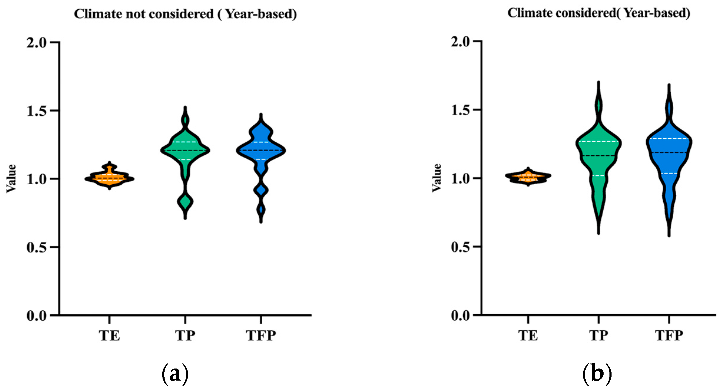
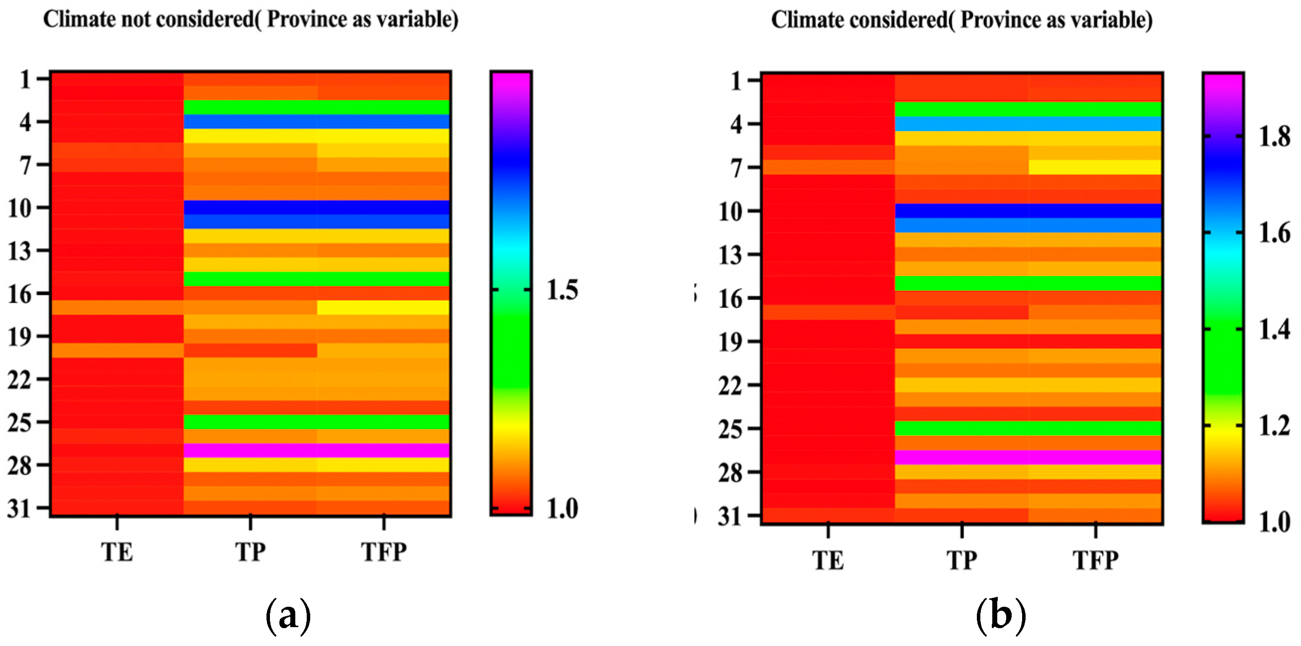
To deeply reveal the heterogeneous impact mechanisms of extreme climate events on freshwater total factor productivity (TFP), Figure 3 and Figure 4 employ a combined visualization analysis of box plots and heat maps. The box plot vividly presents the distribution characteristics of Technical Efficiency (TE), Technical Progress (TP), and Total Factor Productivity (TFP) for each province after incorporating climate variables (such as the number of extreme low temperature days (LTD), extreme high temperature days (HTD), extreme rainy days (ERD), and extreme drought days (EED)). By detailing the interquartile range, it highlights the degree of dispersion in regional differences. The heat map, on the other hand, intuitively maps the response intensity of productivity across the 31 provinces under climate shocks through a gradient of color scales. This integrated visualization approach reveals provincial-level productivity variations under extreme climates, providing a scientific basis for policy formulation.

4. Discussion

4.1. China’s Fisheries’ TFP with and Without Consideration of Climate Factors

From

Table 3. Comparative analysis of Technical Efficiency and Technical Progress changes in freshwater aquaculture: considering vs. not considering climate factors (2000–2023).

	Considering Climate Factors			Not Considering Climate Factors
Year	TE Change	TP Change	TFP Change	TE Change	TP Change	TFP Change
2000	1.00758	0.86454	0.87110	1.08855	0.84374	0.91846
2001	1.00758	0.86454	0.87110	1.08855	0.84374	0.91846
2002	0.97552	0.76873	0.74991	0.96382	0.80495	0.77583
2003	1.03746	1.24526	1.29190	1.02258	1.27916	1.30804
2004	0.98942	1.26726	1.25385	1.00465	1.26809	1.27398
2005	1.00153	1.28083	1.28278	1.00556	1.16284	1.16931
2006	1.03421	0.98136	1.01493	0.99782	1.19583	1.19322
2007	0.97166	1.12808	1.09612	0.99178	1.19288	1.18308
2008	0.98841	1.53043	1.51269	0.96566	1.43061	1.38148
2009	1.05183	1.09094	1.14748	1.06275	1.14434	1.21615
2010	0.98405	1.23953	1.21976	0.99545	1.22437	1.21880
2011	1.02489	1.31108	1.34370	0.97859	1.27022	1.24302
2012	1.00827	1.12076	1.13002	1.03093	1.20694	1.24426
2013	0.98617	1.13349	1.11781	0.98512	1.23571	1.21732
2014	1.01934	0.98175	1.00073	1.00277	1.08072	1.08371
2015	1.01962	0.99480	1.01432	1.03697	1.02388	1.06172
2016	1.01321	1.23237	1.24865	0.99748	1.13956	1.13669
2017	1.00306	1.13754	1.14101	1.03028	1.21503	1.25182
2018	0.97709	1.34035	1.30965	0.97923	1.21628	1.19102
2019	1.02426	1.14414	1.17190	1.00509	1.19776	1.20387
2020	1.02058	1.27079	1.29694	1.03618	1.29333	1.34013
2021	1.01665	1.28448	1.30587	1.01869	1.31236	1.33689
2022	0.98053	1.22956	1.20563	0.95976	1.21013	1.16143
2023	1.02906	1.18629	1.22077	1.02847	1.32313	1.36080

Note: TFP = Total Factor Productivity. The final comparative data on Technical Efficiency (TE), Technical Progress (TP), and Total Factor Productivity (TFP) for the 31 provinces in mainland China were derived before and after climate impacts. The data were categorized based on the Eastern, Central, and Western Regions, with averages calculated for the years 2000 to 2023.

and

Table 4. Regional comparison of TE, TP, and TFP changes: impact of climate factors.

	Considering Climate Factors			Not Considering Climate Factors
Region	TE Change	TP Change	TFP Change	TE Change	TP Change	TFP Change
Eastern	1.005697826	1.104726522	1.102146957	1.008344783	1.127364783	1.124585217
Western	1.01306087	1.218157391	1.229787826	1.014455217	1.245805217	1.253250435
Central	1.000272609	1.164719565	1.162572174	0.998545652	1.178083913	1.173782174
Mean	1.006343768	1.162534493	1.164835652	1.007115217	1.183751304	1.183872609

Note: TFP = Total Factor Productivity; TE = Technical Efficiency; TP = Technical Progress.

, it can be observed that the dynamic evolution of Total Factor Productivity (TFP) presents significant structural differences. When the disaster impact index is not included, the average annual growth rate of TFP reaches 2.78%, with a contribution rate of Technical Progress to TFP at 3.15%. In contrast, Technical Efficiency shows a negative growth rate of −0.37. After incorporating the disaster impact index, the annual growth rate of TFP declines to −1.12%, and the contribution rate of Technical Progress drops to −1.84%, while the contribution rate of Technical Efficiency decreases to −0.12%.

From a temporal perspective, extreme shocks exhibit a threshold effect. In the years when the TFP index exceeds 1.05, the proportion without the disaster index reaches 87.5% (21 out of 24 years). After including the disaster index, this proportion drops to 79.2% (19 out of 24 years). Notably, in 2008, the average TFP index decreased from 1.512, when climate factors were not considered, to 1.381 after considering climate factors, a decline of 8.6%. Additionally, the phased growth rates of TFP vary. The average annual growth rate of TFP from 2000 to 2005 decreased from 2.95% to 1.42%, a decline of 1.53%. In contrast, the TFP growth rate from 2016 to 2020 rebounded from 1.25% to 1.297%, yet remains below the traditionally calculated rate of 1.34%.

From the micro-level data fluctuations, it is evident that Technical Progress in freshwater aquaculture is significantly impacted by climate shocks, indicating a high sensitivity. Specifically, the fluctuations in Technical Progress notably exceed those in Technical Efficiency. The abnormal data from 2003 show that, after climate-adjusted measurements, Technical Progress increased from 0.750 to 1.292. This abnormal fluctuation is closely related to the surface water temperature anomalies triggered by a moderate intensity El Niño event during the same period. El Niño induces the simultaneous occurrence of extreme precipitation and drought through an atmosphere–ocean coupling mechanism, leading to a 12% increase in the damage rate of freshwater aquaculture equipment and a decline in the effectiveness of technology application.

The slight improvement in Technical Efficiency after climate adjustment reflects the differential evolution of adaptive strategies. Firstly, this is a result of optimized management pathways, particularly through the widespread application of dynamic density adjustments and disaster early warning systems [24], which facilitated an increase in the TE index from 1.021 to 1.036 in 2020. Secondly, the buffering effect of infrastructure is notable. Coastal provinces exhibit a more significant improvement in TE compared with inland areas, indicating that the buffering effect largely depends on infrastructure (such as the implementation of freshwater salinity monitoring systems in Guangdong province) and the level of financial investment [25]. In addition to the observed growth, TE experienced actual negative growth with declining trends during the periods of 2019–2020 and 2009–2010, revealing its limitations in responding to accumulated climate change pressures, which reflects the challenges of short-term management in alleviating these pressures [1].

The dynamic evolution of TFP shows a significant deviation characteristic. Between 2016 and 2020, the climate-adjusted TFP of 1.297% was significantly lower than the growth rate of 1.340% driven by traditional factor inputs, with the disparity between the two continuing to widen. This may be attributed to factors such as the diminishing elasticity of Technical Progress and the declining marginal returns of management measures. Moreover, frequently encountered extreme climate events, exemplified by the 2020 floods in the Yangtze River Basin, not only prolonged the research and development cycle of climate-resilient freshwater fish varieties but also illustrated the short-term adaptive strategies’ preliminary effects during the period from 2016 to 2018, which is reflected in the rebound growth rate of TFP (rising from 1.25 to 1.30) [26]. However, with the onset of heatwaves from 2019 to 2020, heightened climate pressures began to diminish the effectiveness of these strategies [27].

In addition, it is worth noting that beyond the climate indicators examined in this study (EDD, HTD, ERD, and LTD), previous research has shown that the dynamic changes in total factor productivity (TFP) may also be influenced by local biotic interactions and time-lagged abiotic conditions. Some studies have suggested that aquaculture processes are better explained by time-lagged ecological variables rather than instantaneous environmental drivers [28,29]. Future research should consider incorporating these potential factors to more comprehensively assess the dynamic impacts of climate change on China’s aquaculture TFP. This would not only enhance the accuracy of evaluations but also provide a stronger scientific basis for developing forward-looking strategies to strengthen the climate resilience of fisheries [30,31].

4.2. Regional Differences in Agricultural TFP Growth with and Without Consideration of Climate Factors

The responsiveness of freshwater fisheries’ TFP to climate factors exhibits significant regional heterogeneity, which can be attributed to the dual impact of Technical Progress and Technical Efficiency. Using the MSBM-DEA model based on provincial panel data from 2000 to 2023, the following key findings emerge:

Firstly, the decline in Technical Progress (TP) in the eastern regions is lower than the national average by 2.7%, a mechanism consistent with the threshold effect model of climate technology diffusion. For instance, in Fujian Province, the salinity adaptive monitoring system utilizes IoT technology to stabilize salinity fluctuations caused by extreme rainfall within a range of ±5‰ [25], thereby reducing the loss rate of Technical Progress to 2.3%, ultimately mitigating the efficiency loss in technology applications. In contrast, inland provinces experience more severe declines in TP, with reductions in Gansu and Tibet reaching 5.5% and 3.4%, respectively. In Gansu, prolonged drought has progressively diminished freshwater sources, causing the operating costs of recirculating freshwater aquaculture systems to remain high. In Tibet, the high salinity evaporation environment of salt lakes (salinity > 50‰) further diminishes the survival of conventional freshwater fish species [32], exacerbating the lag in Technical Development. This regional disparity highlights a core mechanism: coastal zones can mitigate the impact of climate change through technology-intensive infrastructure, whereas inland regions face significantly increased marginal costs of Technical Progress due to resource limitations.

Secondly, Technical Efficiency (TE) exhibits regional differentiation, indirectly reflecting disparities in regional management capabilities. Coastal provinces like Liaoning and Guangdong have shown improvements in TE, which can be attributed to optimized management strategies that partially offset climate pressures. For instance, in Liaoning, the coverage of disaster early warning systems increased from 50% in 2015 to 80% in 2020 [1]. Enhanced timeliness in risk warnings reduced damage rates to freshwater aquaculture facilities during heavy rainfall by 25%, raising TE to 1.036. However, inland provinces have experienced a decline in TE, with significant reductions observed in Guizhou and Qinghai. In Guizhou, the frequency of mudslides reached as high as 12 occurrences [33], yet the adoption rate of systematic climate training among local freshwater aquaculture practitioners remains below 10%. Consequently, disaster response strategies rely primarily on traditional experience.

Thirdly, the distribution of freshwater fisheries’ TFP exhibits a pattern of “stability in the east, decline in the west.” The eastern provinces, supported by technical and policy safeguards, have controlled TFP declines within 3.1%, lower than the national average decline of −5.2%. This is primarily attributable to dual protection from technology and policy. Conversely, the northwestern and southwestern inland provinces show significant sharp declines in TFP, such as Xinjiang (from 1.165 to 1.141, a decline of −2.1%) and Ningxia (from 1.076 to 1.015, a decline of −5.7%). These declines are closely related to systemic deficiencies in resources, technology, and management. In Ningxia, extreme freshwater scarcity forces a reliance on the tributaries of the Yellow River for water supply, with the average number of days of river flow interruption increasing significantly from 30 days in 2010 to 75 days in 2020 [34]. This change has severely hindered the stable application of large-scale freshwater aquaculture technologies. Additionally, from the perspective of extreme climate change, the evaporation rate in arid regions of Xinjiang is three to five times higher than the precipitation rate, leading to excessive salinity in freshwater bodies that reduces the efficiency of conventional technologies. Such regional disparities fundamentally reveal the gradient differences in climate adaptability. Coastal regions maintain technical resilience through substantial investment, whereas inland areas, constrained by various limitations, are caught in a “low-tech equilibrium trap.”

Fourthly, from a comprehensive perspective, the impact of Technical Efficiency (TE) and Technical Progress (TP) on total factor productivity (TFP) reveals a phenomenon of “localized improvement, overall stagnation.” Specifically, in some provinces, such as Liaoning, improvements in TE partially offset the pressures exerted by climate change, demonstrating the potential role of TE enhancement in mitigating climate shocks. Liaoning occupies a significant position in national freshwater aquacultures; although its output and value are not comparable to some traditional coastal provinces, its development potential remains promising. The province’s industrial layout is rational, and data analysis shows that its TE improved from 1.069 to 1.102. Based on this, it can be preliminarily inferred that the enhancement of TE in Liaoning’s freshwater aquaculture may be attributed to the adoption and promotion of engineered recirculating freshwater aquaculture systems and infrastructure upgrades, such as standardized renovations of freshwater aquaculture ponds.

5. Conclusions

The empirical research based on the MSBM-DEA model indicates that climate change has a significant structural impact on the Total Factor Productivity (TFP) of freshwater fisheries. In the baseline model that does not consider climate factors, the average annual growth rate of TFP is 2.78%, with the contribution rate of Technical Progress being 3.15%. However, when extreme climate events (such as extreme temperatures, precipitation, and drought) are introduced as core explanatory variables, the TFP growth rate declines to 1.12%, the contribution rate of Technical Progress drops to 1.84%, and Technical Efficiency shows only a slight improvement of 0.37%, failing to offset the cumulative effects of climate shocks.

From a regional perspective, the TFP of freshwater fisheries exhibits a dual characteristic of resilience in the eastern regions and vulnerability in the inland areas. The eastern provinces, such as Fujian and Shandong, demonstrate strong adaptive capacities through technology-intensive initiatives and policy synergies. The widespread implementation of infrastructure like salinity adaptive monitoring systems and disaster early warning networks helps limit the suppression of Technical Progress to less than 3%. Additionally, fiscal subsidies and automated management systems (such as the feeding systems in Zhejiang) enhance the stability of Technical Efficiency.

In contrast, the northwestern and southwestern provinces, such as Gansu and Guizhou, face dual constraints from natural endowments and management shortcomings. Long-term drought conditions have led to the shrinkage of freshwater ecosystems, notably reflected in the significant reduction in their coverage area. Furthermore, the cumulative effects of extreme climate events, such as mudslides triggered by abnormal rainfall and salinity imbalances, generally result in a decline in Technical Progress exceeding 5%. In inland regions, the inadequate training on climate change for freshwater aquaculture practitioners and the lack of skilled personnel with fisheries expertise exacerbate the deterioration of Technical Efficiency, with areas like Qinghai experiencing a decline of 7.2%.

While this study reveals the significant suppressive effect of climate shocks on the total factor productivity (TFP) of freshwater fisheries through a dynamic MSBM-DEA model, it remains subject to dual limitations in theoretical construction and empirical analysis. Firstly, the selection of climate variables suffers from bias; the current model only incorporates four direct climate indicators—extreme low temperatures, extreme high temperatures, abnormal precipitation, and drought—while neglecting indirect risk factors such as floods, typhoons, and saltwater intrusion caused by rising sea levels. This selection bias in indicators may lead to an underestimation of extreme climate factors, potentially resulting in a multiplicative effect on TFP losses. Future research should build upon the existing studies to develop a multidimensional Disaster Impact Index (DII) to comprehensively and thoroughly capture the complexity and multidimensional characteristics of climate risks.

China’s experience indicates that enhancing the climate adaptability of freshwater aquaculture requires focusing on three key actions: differentiated technical innovation, regional governance collaboration, and international knowledge transfer. The study findings show that eastern regions, underpinned by technical advances and policy support, demonstrate a strong adaptive capacity, while inland areas encounter significant vulnerability. This disparity indicates that climate adaptation strategies should be customized to regional circumstances. Eastern regions can leverage intelligent and modern monitoring systems to mitigate the impact of extreme climate events on production efficiency, whereas inland regions must strengthen infrastructure and management capabilities to enhance the effectiveness of technology application.

Moreover, the importance of regional governance collaboration cannot be overemphasized. The eastern provinces have effectively improved Technical Efficiency by optimizing management strategies and enhancing disaster warning systems, providing useful lessons for other regions. Facilitating experience sharing and collaborative governance across regions will contribute to enhancing the overall resilience of freshwater aquaculture.

As the world’s largest aquaculture nation, particularly in freshwater aquaculture, China’s practices not only offer a low-cost adaptation pathway for developing countries but also provide empirical support for global climate governance frameworks. By strengthening cooperation and communication with the international community and learning from advanced technologies and management experiences, China is poised to achieve a sustainable transition in aquaculture productivity amid the climate crisis, safeguarding the resilient future of the “blue granary.” It is only through the deep integration of local innovations with global cooperation that the challenges posed by climate change can be effectively addressed, propelling the long-term development of freshwater aquaculture.