The Effect of Ontogenetic Dietary Shifts on the Trophic Structure of Fish Communities Based on the Trophic Spectrum

Abstract

The trophic spectrum provides a useful method to investigate the trophic structure of fish communities. However, ontogenetic shifts in diet can cause variations in the trophic level with body size, thereby influencing the trophic structure of fish communities. In this study, we investigated the effect of ontogenetic dietary shifts on the trophic structure of fish communities in Haizhou Bay based on trophic spectra and trophic indicators calculated under different scenarios of functional group classification. The results showed that the size threshold of ontogenetic dietary shifts was a viable basis for functional group classification. The biomass of fishes at trophic levels 3.4–3.8 was lower when ontogenetic dietary shifts were considered, which can influence the intensity of top–down control and hinder the formulation of harvest strategies. Ontogenetic dietary shifts can also redistribute the biomass of fishes across trophic levels, thereby regulating the trophic structure of fish communities. Different responses of trophic indicators to ontogenetic dietary shifts were identified, with high trophic indicator (HTI) being the most appropriate indicator reflecting the effect of ontogenetic dietary shifts in the trophic structure. This study provides a feasible way to optimize the trophic spectrum for elucidating the trophic structure of fish communities. And we recommend that ontogenetic dietary shifts should be considered and valued in fishery management.

1. Introduction

Trophodynamics is a vital aspect of ecosystem dynamics [1,2], providing insights into the trophic position of individuals [3] and the trophic structure of catches [4], which have been widely applied in fishery science and management [5,6]. Trophic relationship is not only one of the key factors determining the variation of fish stock abundance and productivity [7], but also the base for ecosystem modeling studies [8] and the implementation of ecosystem-based fishery management [9].

Functional group division has often been applied to ‘simplifying food webs’ in the research of trophodynamics [10], which requires high consistency of parameters within each functional group [11]. Typically, the division of functional groups mainly focuses on the diet similarity among species [12,13,14], with limited considerations of individual-level differences, such as the ontogenetic dietary variations of species. Body size is a key parameter when investigating trophic interactions in fish communities [15]. The relationship between fish size and food composition varies across species [16,17]. Thus, neglecting the size structure of fish may mask changes in trophic interactions, and lead to unrealistic and biased conclusions for the trophic structure of fish communities.

The trophic spectrum is a two-dimensional graph with the trophic level as the horizontal axis, and biomass, catch or abundance as the vertical axis, which can reflect communities through biomass at different trophic levels [15]. This approach enables the visualization and analysis of variations in biomass of communities by trophic level, making it an effective method to evaluate the impact of fishing pressure and climate changes on the trophic structure of fish communities [18,19,20]. In the trophic spectrum, fish communities are aggregated by biomass of different trophic level classes, and the information on species is hidden, whereby feeding and growth processes could be represented based on the changes in the biomass distribution of trophic levels [15], and fish species with different ontogenetic stages can be shown as biomass at different trophic levels. As such, the trophic spectrum provides a preferred method for investigating the effect of ontogenetic dietary shifts on the trophic structure of fish communities.

Haizhou Bay is a typical open bay located in the middle Yellow Sea of China. It is one of important spawning, feeding and nursery grounds for many fish species in the Yellow Sea [21]. In the face of intense fishing pressure and climate changes over recent decades [21,22,23], fish communities in Haizhou Bay have shown obvious trends of reduced stability [24] and a decrease in large-sized individuals [25], both of which have indicated high demand for effective fishery management of the size structure. The observed changes in species composition and size structure within the fish community of Haizhou Bay provide valuable insights into the effects of ontogenetic dietary shifts in an overexploited ecosystem.

In this study, the effect of ontogenetic dietary shifts on the trophic structure of fish communities in Haizhou Bay was assessed through comparisons of trophic spectra across different scenarios (with or without considering the size structure). Three indicators, including the mean trophic level, high trophic indicator, and slope of the trophic spectrum, were also calculated to further investigate the effect of ontogenetic dietary shifts. By using the trophic spectrum and indicators, our study intends to solve the following questions: (1) how can we classify functional groups based on fish size to reflect the effects of ontogeny, (2) what is the effect of ontogenetic dietary shifts on the trophic structure of an actual fish community, and (3) what can we learn to optimize fishery management when ontogenetic dietary shifts are considered. This study provided a feasible method to elucidate the trophic structure of fish communities in marine ecosystems.

2. Materials and Methods

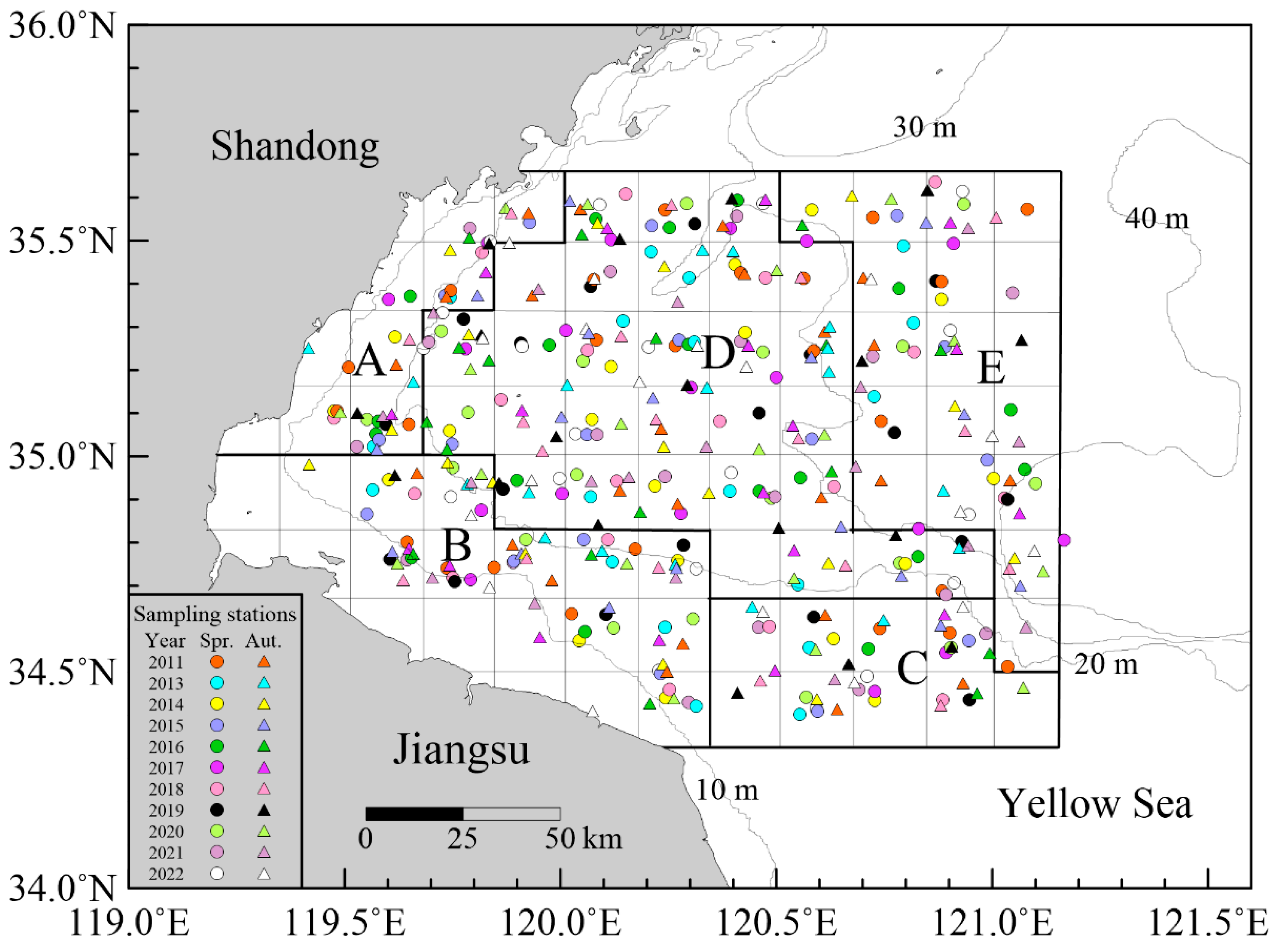
2.1. Sample Collection

Samples were collected by bottom trawl surveys in the spring (April–May) and autumn (September–October) of 2011 and 2013–2022 in Haizhou Bay and adjacent waters in China. Stratified random sampling was conducted, with stations covering five sub-regions with distinct depths and geographic locations (A–E) of the sampling area [26] (Figure 1). The number of stations was 24 in 2011, and was adjusted to 18 from 2013 to 2022 because of the optimization of sampling. This optimization required that the stations of each voyage cover the 5 sub-regions, which could offset the loss of survey estimate precision caused by the decrease in sampling effort and reduce the cost of the survey and the negative impacts of survey trawling on low-abundance species [26].

At each station, a bottom trawl survey was conducted for approximately one hour at a speed of 2–3 knots. The power of fishing boats was about 220 kW, with the net width of 25 m and the cod-end mesh of 17 mm. The samples were analyzed in the laboratory, and biological data were measured and recorded. Fishing efforts were standardized with a trawl speed of 2 knots (i.e., 3.704 km/h) and an operation time of 1 h for each station. The biomass of each fish species at each station was calculated as follows:

$$C_{ij}^{\prime }={\displaystyle \frac{60}{t_i}}\times {\displaystyle \frac{3.704}{v_i}}\times C_{ij}$$

$$B_{ij}={\displaystyle \frac{C_{ij}^{\prime }}{a{q}_j}}$$

where $C_{ij}^{\prime }$ (kg/h) is the standardized catch of fish species j in station i, 60 is the operation time (min) of standardized fishing effort, $t_i$ (min) is the actual operation time of station i, 3.704 (km/h) is the trawl speed of standardized fishing effort, $v_i$ (km/h) is mean trawl speed during the survey of station i, $C_{ij}$ (kg) is the actual catch of fish species j in station i, $B_{ij}$ (kg/km²) is the biomass of fish species j in station i, $a$ (km²) is the area swept by trawl at each station when fishing effort was standardized as above and herein is 0.0926 km², and $q_j$ is the catchability coefficient of fish species j.

Different catchability coefficients were set between 0.3 and 1.0 to estimate the relative biomass of different fish species [27]. For demersal fish species with weak swimming ability, the catchability coefficient was set at 0.8–1.0. For fish species of which the swimming ability was between that of pelagic and demersal fish, the catchability coefficient was set as 0.5. For pelagic fish species, the catchability coefficient was set as 0.3 [27].

Further, the biomass of fish species j in each voyage was calculated as the arithmetic average biomass of fish species j across all stations investigated during the voyage.

2.2. Functional Group Classification

To identify the dominant species and appropriately classify the functional group, the biomass proportion of each fish species in the fish communities (i.e., relative biomass) was calculated using samples from all voyages in all years. Diverse characteristics of food acquisition were observed among fish species in Haizhou Bay [24], which reflected the different roles of species within the trophic structure of fish communities. To ensure that the research can capture as many characteristics as possible and control the model complexity, each fish species with relative biomass exceeding 0.50% was classified into one functional group when ontogenetic dietary shifts were not considered.

For each species without distinct ontogenetic dietary shifts, symmetrical distribution of biomass is considered reasonable and one functional group is classified. For species with distinct ontogenetic dietary shifts, their trophic levels are not symmetrical around the mean trophic level of the species and more detailed classification of functional groups should be carried out.

In this study, six fish species with distinct ontogenetic dietary shifts were selected to explore the influence of these shifts on the trophic spectrum. Each of the species was further classified into different functional groups according to different scenarios considering the size structure (

Table 1. Dietary shift thresholds and equidistant size classes for six fish species with distinct ontogenetic dietary shifts in Haizhou Bay.

Species	Size Thresholds of Dietary Shift (cm)	Equidistant Size Classes (cm)
		Range of Size	Size Interval
Hexagrammos otakii	80, 130 [28]	50–150	10
Cynoglossus joyneri	184 [29]	65–195	10
Saurida elongata	180 [30]	60–180	10
Chelidonichthys spinosus	150 [31]	110–150	10
Larimichthys polyactis	110 [32]	90–130	10
Collichthys lucidus	70 [33]	40–120	10

Note: Total length was used for Cynoglossus joyneri and standard length was used for other fish species.

). scenarios were set as follows: (A) size structures were not considered and each species was classified into one functional group; (B) species with distinct ontogenetic shifts were classified into different functional groups based on dietary shift thresholds of body size [28,29,30,31,32,33]; and (C) ontogenetic dietary shifts were considered to occur gradually and species with distinct ontogenetic shifts were classified into different functional groups based on equidistant size classes. The ranges of equidistant size classes were determined based on the fish size of isotope samples. Moreover, 10 cm was a common interval used for cluster analysis to determine the size thresholds of dietary shifts (e.g., Xu et al. [28]), and was used as the size interval of equidistant size classes.

These scenarios will mimic the variations in trophic levels across different developmental stages within the same species and reflect the different roles of these species in the context of whether and how ontogenetic dietary shifts occurred.

2.3. Stable Isotope Analysis and Trophic Level

A total of 239 specimens of different fish species collected from the sampling area in 2018 were used for stable isotope analysis. For each specimen, the white muscles near the first dorsal fin of individuals were sampled for stable isotope analysis. The analysis was carried out at the Institute of Hydrobiology of Chinese Academy of Sciences, and a stable isotope mass spectrometer was applied to measure the stable isotope ratios of nitrogen (δ¹⁵N). The stable isotope ratios were calculated as follows:

$${\delta }^{15}N=1000\times \left({\displaystyle \frac{15N/{14N}_s-15N/{14N}_a}{15N/{14N}_a}}\right)$$

where $15N/{14N}_s$ is the nitrogen stable isotope ratio of samples, $15N/{14N}_a$ is the nitrogen stable isotope ratio of standard matter (atmospheric nitrogen).

The trophic level of each functional group was calculated using data from stable isotope analysis and supplemented with information obtained from the literature [25,34,35,36]. The formula is as follows:

$$TL=2+{\displaystyle \frac{{{\delta }^{15}{N}_s-\delta }^{15}{N}_b}{k}}$$

where TL is the trophic level of fish, ${\delta }^{15}{N}_s$ is the stable isotope ratio of sample, ${\delta }^{15}{N}_b$ is the stable isotope ratio of baseline, and k is the difference of ${\delta }^{15}\mathrm{N}$ between two adjacent trophic levels. In this case, k is 3.40‰ [37]. The baseline should be primary consumers with few changes in the trophic level. Azumapecten farreri collected in the bottom trawl surveys was chosen as the baseline species, with a ${\delta }^{15}\mathrm{N}$ value of 4.46‰.

2.4. Trophic Spectrum

On the trophic spectrum, the biomass of a trophic level is calculated as the sum of each functional group at this trophic level. Here, trophic spectra were, respectively, constructed based on three scenarios (scenarios (A)–(C)), where species with distinct ontogenetic dietary shifts were classified into different functional groups with or without considering the size structure of them. Further, the proportion of the biomass of the six species with distinct ontogenetic dietary shifts in each voyage in each trophic level was studied to identify the role of these species in the trophic structure of fish communities.

The trophic spectra of fish communities in Haizhou Bay during the spring and autumn of 2011 and 2013–2022 were constructed using package ‘EcoTroph’ [38] in R software (version 4.3.2) [39]. It was assumed that the biomass of each functional group followed a lognormal distribution around their mean trophic level, with a sigma value of 0.12 applied to the lognormal distribution [38]. The functions ‘create.smooth’ and ‘Transpose’ from R package ‘EcoTroph’ [38] were used to calculate the biomass at intervals of 0.1 trophic levels (i.e., Δτ = 0.1). R package ‘ggplot2’ [40] was applied to draw graphs of the trophic spectra.

2.5. Trophic Indicators

To investigate the variations in the trophic structure of fish communities in Haizhou Bay, three trophic indicators were calculated to reflect the status of fish communities.

(a) Mean trophic level (MTL). MTL is the mean trophic level of fishes weighted by their biomass, which is widely applied in the analysis of trophodynamics and could be used to examine the status of marine ecosystems [41]. MTL is an appropriate indicator to reflect the structure of fish communities from the perspective of whole communities [42].

(b) High trophic indicator (HTI). HTI is the proportion of high-trophic-level organisms with trophic level higher than 4.0 [43,44], which can reflect the impacts of fishing pressure on fish communities [43]. Species with high trophic levels tend to show important roles in stability of ecosystems [45], and HTI will provide useful information on the abundance of these species.

(c) Slope of the trophic spectrum (slope). Similar to the slope of the size spectrum, slope of the trophic spectrum is the coefficient of a linear regression equation with logarithmic biomass as the dependent variable and trophic level as the independent variable [43]. The slope can reflect the relationship of biomass at each trophic level. A flatter slope indicates a higher proportion of high-trophic-level individuals in fish communities, which can be regarded as a higher stability of fish communities [44], especially in overexploited ecosystems. In this study, the calculation of slope begins at the trophic level 3.0 and ends at the trophic level 5.0 to avoid the inaccessible part of trawl surveys [43], and 10 was chosen as base of the logarithm to be consistent with Lindeman’s efficiency [46].

To test the temporal trend of the three indicators, Mann–Kendall tests and Sen’s slopes were performed. The Mann–Kendall test is a non-parametric method that does not require data to follow a specific distribution [47,48] and has been widely applied for detecting trends in time series data (e.g., Kale [49]). Sen’s slope [50] was utilized to estimate the variation in indicators to prevent the effect of outliers.

3. Results

3.1. Relative Biomass and Trophic Levels of Fish Species

A total of 116 fish species were analyzed. The biomass of different species showed obvious variations, with Chelidonichthys spinosus demonstrating a relatively high biomass of 849.21 kg/km² and Salanx longianalis exhibiting a relatively low biomass of less than 0.01 kg/km². In this study, 31 species with a relative biomass exceeding 0.50% were classified into separate functional groups, and they accounted for 94.11% of the total fish biomass, while the remaining fish species were grouped into the “others” category (

Table 2. Catchability coefficient, relative biomass, trophic levels, and analytical method for trophic levels of fish species in Haizhou Bay.

Fish Species	Catchability Coefficient	Relative Biomass (%)	Trophic Level	Analytical Method
Chelidonichthys spinosus	0.5	14.70%	3.88	SIA (this study)
Enedrias fangi	0.5	13.59%	3.24	SCA [25]
Larimichthys polyactis	0.5	11.73%	3.83	SIA (this study)
Thryssa kammalensis	0.3	9.54%	3.20	SCA [34]
Pampus argenteus	0.3	4.83%	3.25	SCA [25]
Saurida elongata	0.5	4.34%	4.15	SIA (this study)
Liparis sp.	0.5	4.00%	3.86	SIA (this study)
Hexagrammos otakii	0.5	3.23%	3.69	SIA (this study)
Collichthys lucidus	0.5	2.76%	3.64	SIA (this study)
Conger myriaster	0.5	2.48%	4.22	SCA [25]
Lophius litulon	0.8	2.11%	4.36	SCA [25]
Syngnathus acus	0.5	1.83%	3.20	SCA [25]
Miichthys miiuy	0.5	1.70%	4.16	SCA [25]
Engraulis japonicus	0.3	1.58%	3.60	SCA [34]
Setipinna tenuifilis	0.3	1.56%	3.28	SIA [35]
Cynoglossus joyneri	1.0	1.50%	3.55	SIA (this study)
Callionymus valenciennei	0.5	1.41%	3.72	SIA (this study)
Johnius belengeri	0.5	1.28%	3.83	SCA [25]
Collichthys niveatus	0.5	1.21%	3.35	SIA (this study)
Trichiurus lepturus	0.5	0.96%	4.78	SCA [25]
Ammodytes personatus	0.5	0.94%	3.37	SCA [25]
Argyrosomus argentatus	0.5	0.87%	4.13	SCA [25]
Apogon lineatus	0.5	0.85%	3.40	SCA [25]
Chaeturichthys stigmatias	0.8	0.79%	3.86	SCA [25]
Platycephalus indicus	0.5	0.75%	3.93	SIA [35]
Muraenesox cinereus	0.5	0.65%	3.68	SIA (this study)
Callionymus beniteguri	0.5	0.64%	3.36	SCA [25]
Callionymus kitaharae	0.5	0.61%	3.39	SCA [25]
Pleuronichthys cornutus	1.0	0.60%	3.53	SCA [25]
Amblychaeturichthys hexanema	0.8	0.58%	3.88	SIA (this study)
Callionymus richardsoni	0.5	0.50%	3.53	SCA [25]
Others	0.5	5.89%	3.70	Ecopath [36]

Note: Trophic levels are based on scenarios without ontogenetic dietary shifts (i.e., scenario A). SCA: stomach content analysis, SIA: stable isotope analysis.

). Notably, the biomass of the six species with distinct ontogenetic dietary shifts accounted for 36.54% of the total fish biomass in Haizhou Bay.

Nitrogen stable isotope values varied among different species (

Table A1. Sample size and δ¹⁵N of fish species for the stable isotope analysis in Haizhou Bay in 2018.

Fish Species	Number of Samples	δ15N (‰, Mean ± SD)
Chelidonichthys spinosus	18	10.85 ± 0.64
Larimichthys polyactis	27	10.80 ± 0.86
Saurida elongata	27	11.67 ± 1.37
Liparis sp.	4	10.37 ± 1.02
Hexagrammos otakii	33	10.07 ± 1.58
Collichthys lucidus	41	9.81 ± 1.74
Cynoglossus joyneri	63	9.48 ± 1.41
Callionymus valenciennei	7	10.31 ± 1.06
Collichthys niveatus	6	9.03 ± 1.65
Muraenesox cinereus	6	10.17 ± 1.23
Amblychaeturichthys hexanema	7	10.84 ± 1.04
Total	239	-

). The trophic levels of fish species in Haizhou Bay ranged from 3.20 to 4.78, with the majority of species occupying trophic levels between 3.20 and 4.00 (Table 2). Fish communities in Haizhou Bay were predominantly composed of small-sized fish species, such as Enedrias fangi and Thryssa kammalensis.

Six species with distinct ontogenetic dietary shifts varied greatly in nitrogen isotope values among different size classes (

Table A2. Sample size and δ¹⁵N of each size class of the six species with distinct ontogenetic dietary shifts for the stable isotope analysis in Haizhou Bay in 2018.

Species	Size Classes	Number of Samples	δ15N (‰, Mean ± SD)
Chelidonichthys spinosus	<111	3	11.05 ± 0.95
	111–120	3	11.05 ± 0.62
	121–130	3	11.32 ± 0.51
	131–140	3	10.20 ± 0.47
	141–150 *	3	10.89 ± 0.53
	>151	3	10.59 ± 0.28
	Subtotal	18	10.85 ± 0.64
Collichthys lucidus	<41	1	7.98
	41–50	3	8.11 ± 1.04
	51–60	6	8.60 ± 1.50
	61–70 *	4	9.42 ± 0.70
	71–80	7	10.50 ± 1.02
	81–90	6	10.10 ± 0.40
	91–100	5	11.51 ± 1.31
	101–110	5	11.62 ± 1.14
	111–120	3	9.47 ± 0.53
	>121	1	10.89
	Subtotal	41	9.81 ± 1.74
Cynoglossus joyneri	<65	3	8.69 ± 0.71
	65–74	4	9.69 ± 0.40
	75–84	8	9.22 ± 1.22
	85–94	4	9.26 ± 1.48
	95–104	2	8.68 ± 0.55
	105–114	6	9.38 ± 1.04
	115–124	4	11.13 ± 1.11
	125–134	4	9.86 ± 0.93
	135–144	4	9.50 ± 0.28
	145–154	4	8.80 ± 1.79
	155–164	8	9.06 ± 1.21
	165–174	3	10.45 ± 1.47
	175–184 *	3	10.80 ± 0.72
	185–194	3	11.43 ± 0.42
	>195	3	11.65 ± 0.51
	Subtotal	63	9.48 ± 1.41
Hexagrammos otakii	<51	1	9.68
	51–60	6	9.15 ± 1.40
	61–70	1	7.81
	71–80 *	1	11.14
	81–90	3	11.56 ± 0.55
	91–100	3	9.65 ± 0.38
	101–110	4	10.61 ± 0.34
	111–120	3	10.68 ± 1.10
	121–130 *	3	9.02 ± 1.03
	131–140	4	10.65 ± 2.29
	141–150	3	11.25 ± 0.31
	>151	1	11.44
	Subtotal	33	10.07 ± 1.58
Larimichthys polyactis	<91	3	10.51 ± 0.47
	91–100	3	11.00 ± 1.10
	101–110 *	6	10.28 ± 0.78
	111–120	4	10.65 ± 1.24
	121–130	6	11.13 ± 0.81
	>131	5	10.57 ± 1.65
	Subtotal	27	10.80 ± 0.86
Saurida elongata	<61	2	10.84 ± 1.81
	61–70	2	12.34 ± 0.36
	71–80	2	11.17 ± 0.49
	81–90	3	11.87 ± 0.85
	91–100	3	11.15 ± 1.20
	101–110	3	11.94 ± 0.50
	111–120	1	11.99
	121–130	3	12.08 ± 1.12
	131–140	2	11.32 ± 1.33
	141–150	3	12.30 ± 0.19
	151–180 *	1	12.51
	>180	2	11.94 ± 0.80
	Subtotal	27	11.67 ± 1.37
Total		209	-

Note: * represents that the ontogenetic dietary shifts occurred at the end of the interval.

) and belonged to different trophic levels under three scenarios (Figure 2). Moreover, the δ¹⁵N values of the six species were lower than those of other studies using stable isotope analysis. In general, the trophic levels of these species were higher than the trophic levels reported in these studies, but lower than the trophic levels obtained from stomach content analysis in this area (

Table A3. Comparison of δ¹⁵N and trophic levels of the six species with distinct ontogenetic dietary shifts among different studies.

Fish Species	This Study		Jiaozhou Bay [57]		Lingshan Island [58]		SCA of Haizhou Bay [25]
	δ15N (‰)	TL	δ15N (‰)	TL	δ15N (‰)	TL	TL
Chelidonichthys spinosus	10.85	3.88	11.55	3.28	10.94	3.38	4.08
Collichthys lucidus	9.81	3.64	-	-	11.71	3.60	3.75
Cynoglossus joyneri	9.48	3.55	13.62	3.89	11.24	3.46	3.10
Hexagrammos otakii	10.07	3.69	13.54	3.86	12.86	3.94	3.83
Larimichthys polyactis	10.8	3.83	13.65	3.9	12.18	3.74	4.02
Saurida elongata	11.67	4.15	12.88	3.67	11.56	3.56	4.50

Note: TL: trophic level, SCA: stomach content analysis.

).

The intersection of the line in scenario A (intraspecies dietary variations were omitted) and scenario B (intraspecies dietary variations were assumed to occur before and after ontogenetic dietary shift) was not in the center of the range (Figure 2a). The trophic levels of the six fish increased with size, except for C. spinosus in scenario B, with Saurida elongata having the highest trophic level, while the trophic level of Cynoglossus joyneri showed the greatest variation with ontogeny (0.59). The trophic levels of each size class fluctuated around the mean trophic level in scenario C (intraspecies dietary variations were assumed to occur during the whole ontogeny) (Figure 2b). The trophic level of Hexagrammos otakii varied greatly, ranging from 2.99 to 4.09, while the trophic level of Larimichthys polyactis only showed minor variations (3.71–3.96). Since trophic levels in scenario C fluctuated drastically with ontogeny, we selected scenario B to investigate the variation in the trophic spectrum of fish communities.

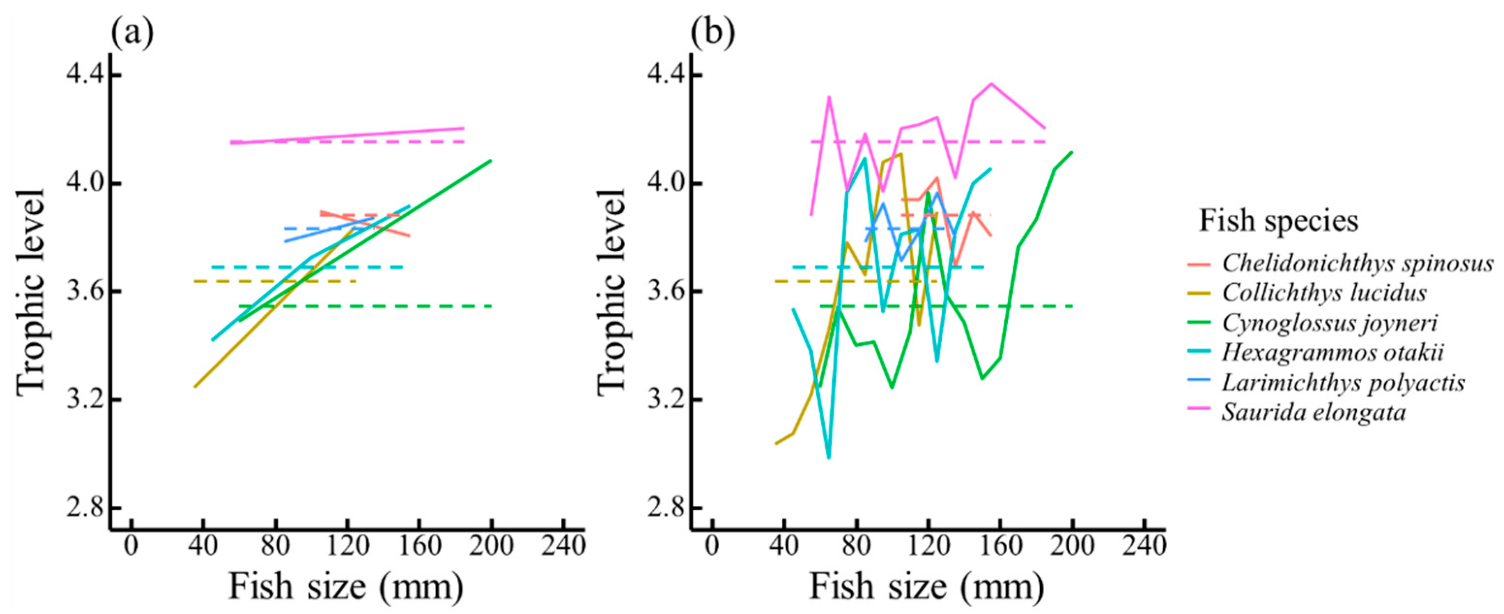
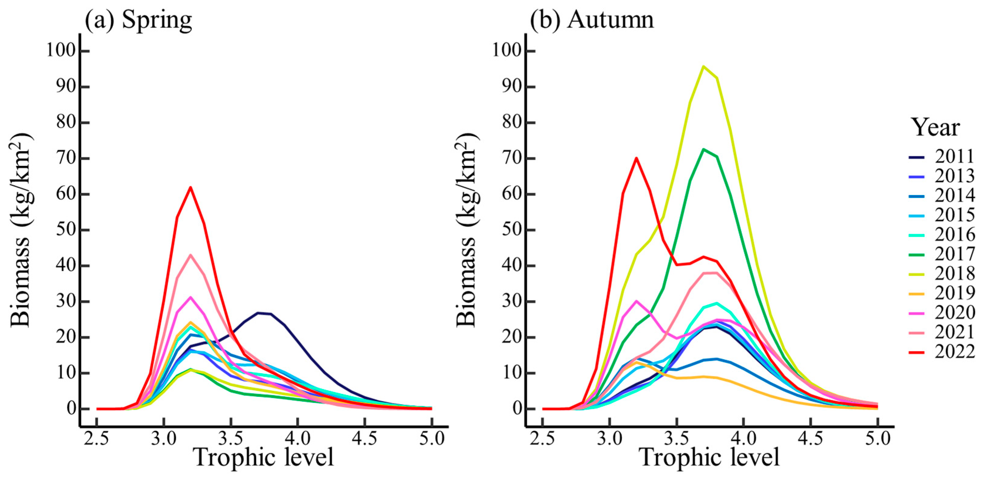
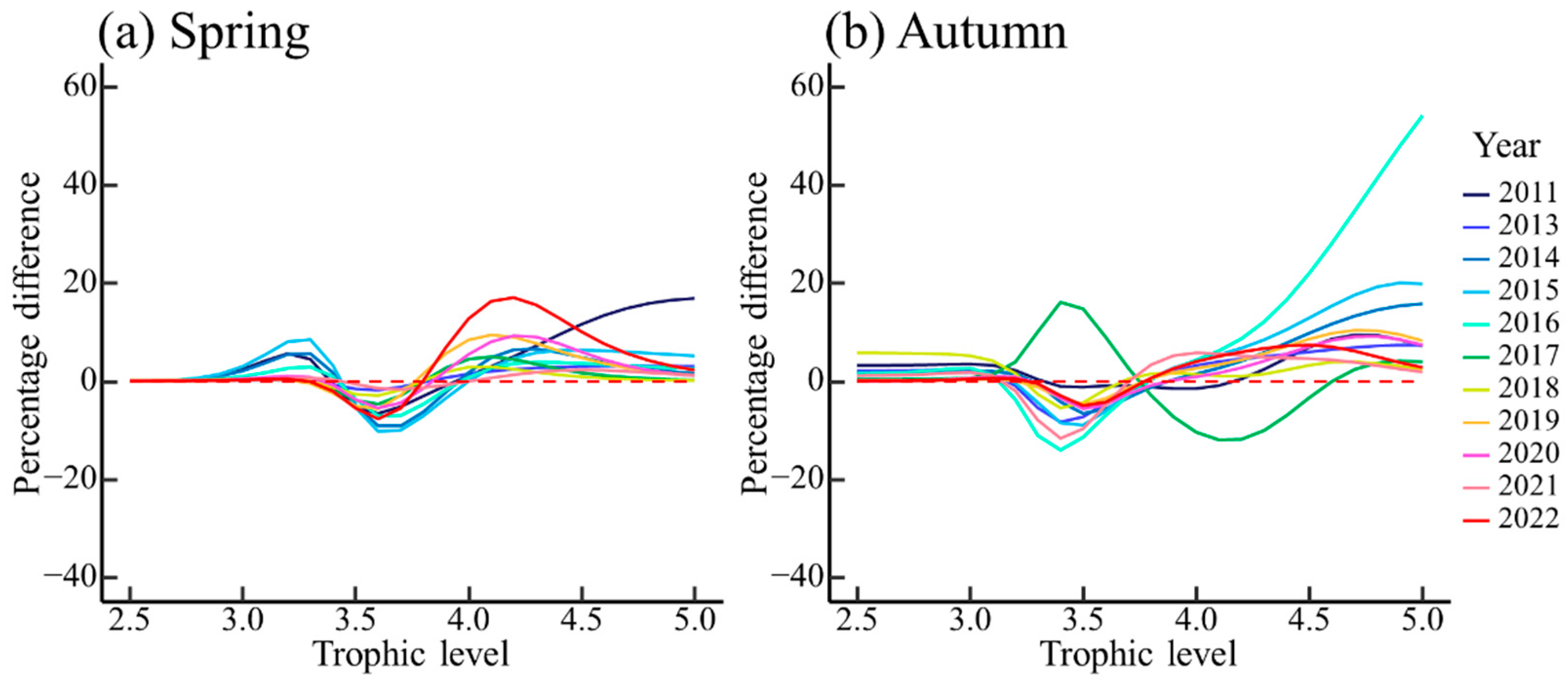
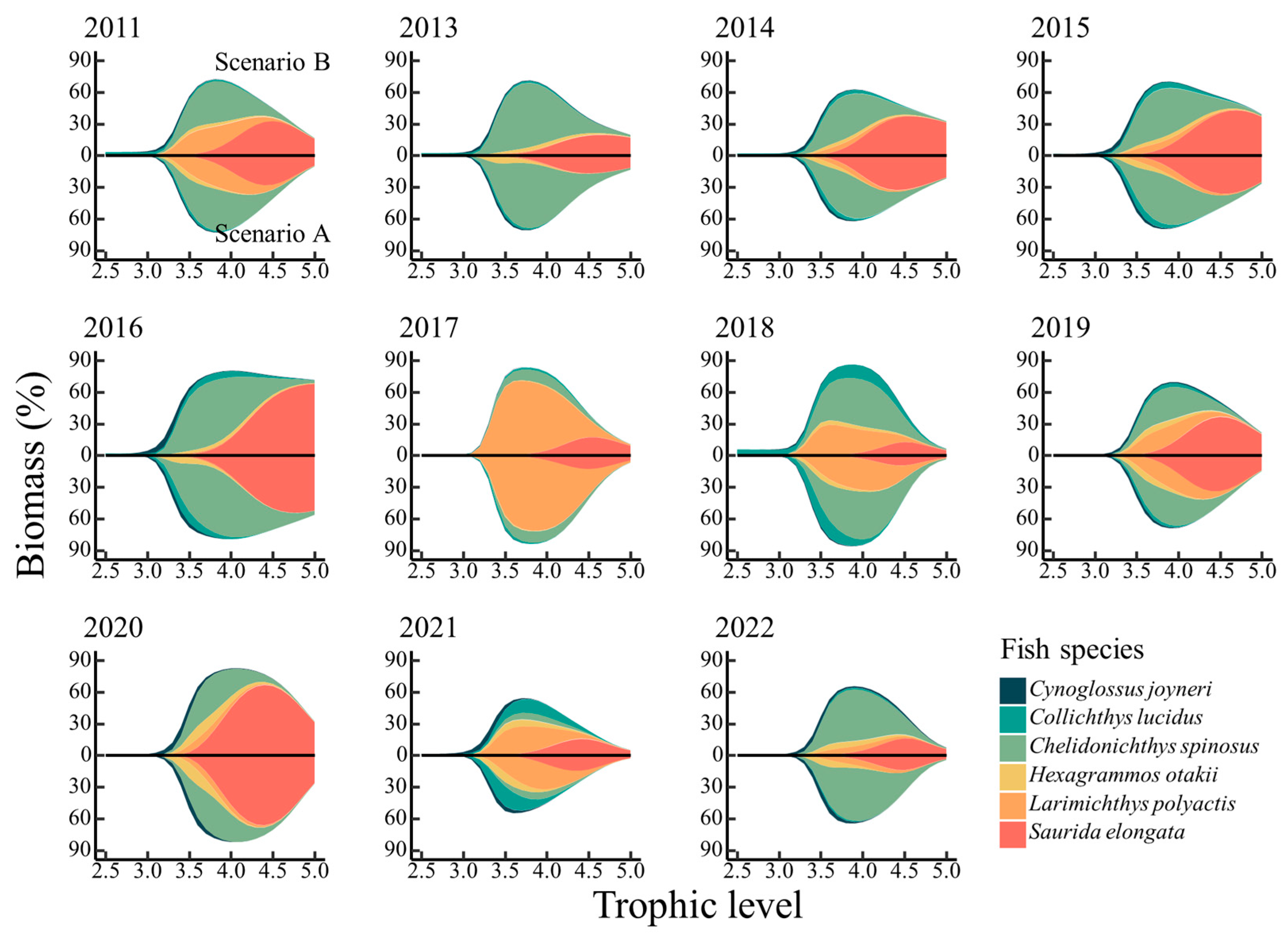
3.2. Effect of Ontogenetic Dietary Variations on the Trophic Spectrum

Obvious differences were observed among biomass in the trophic spectra of fish communities in Haizhou Bay during the spring and autumn of 2011 and 2013–2022 in scenarios A, B and C (Table S1). In scenario B, species with distinct ontogenetic dietary shifts were classified into different functional groups, and the trophic spectra of fish communities in Haizhou Bay were constructed during the spring and autumn of 2011 and 2013–2022 (Figure 3). The shape of trophic spectra showed expected seasonal and annual variations. In spring, the total biomass of fish communities in Haizhou Bay was lower than that in autumn, while the variability in trophic spectra was higher in autumn compared to spring. The biomass of high trophic level fish species was lower in spring, resulting in a lower peak in the trophic spectra compared to autumn. In spring, the peak of the trophic spectrum occurred at a trophic level of 3.7 in 2011, while the peaks of trophic spectra were at a trophic level of 3.2 in other years. In autumn, the peak of trophic spectra were observed at a trophic level of 3.8. Most trophic spectra showed a single peak, while trophic spectra in the autumn of 2014, 2020 and 2022 had a bimodal shape. Notably, in 2017 and 2018, the total biomass of fish was higher in autumn and lower in spring.

Compared to scenario B, the biomass distribution of trophic spectra in scenario A trended to be more concentrated. In this scenario, a higher biomass was observed between trophic levels 3.4 and 3.8, while the biomass was lower across other trophic levels. In autumn, notable differences were observed in 2017, when trophic spectra in scenario B displayed a lower biomass between trophic levels 3.8 and 4.6 (Figure 4).

The proportion of biomass of the six species with distinct ontogenetic dietary shifts was mainly distributed at trophic levels ranging from 3.5 to 4.5, but varied greatly among seasons and years (Figure 5 and Figure 6). In spring, the proportion of biomass of these species was lower than 40% during the study period, and H. otakii had the greatest change when size structure was considered (scenario B). Moreover, in this season, L. polyactis was the main species between trophic levels 3.5 and 4.5, and S. elongata was the species with the highest biomass at a trophic level higher than 4.0 in 2011, 2013, 2015 and 2016 (Figure 5). In autumn, species with distinct ontogenetic dietary shifts had a higher proportion of biomass than in spring, especially between trophic levels 3.6 and 4.3. With C. spinosus, L. polyactis and S. elongata as dominant species, the proportion of biomass of the six species changed mildly between scenarios in autumn, but the composition of species with distinct ontogenetic dietary shifts at each trophic level showed differences (Figure 6).

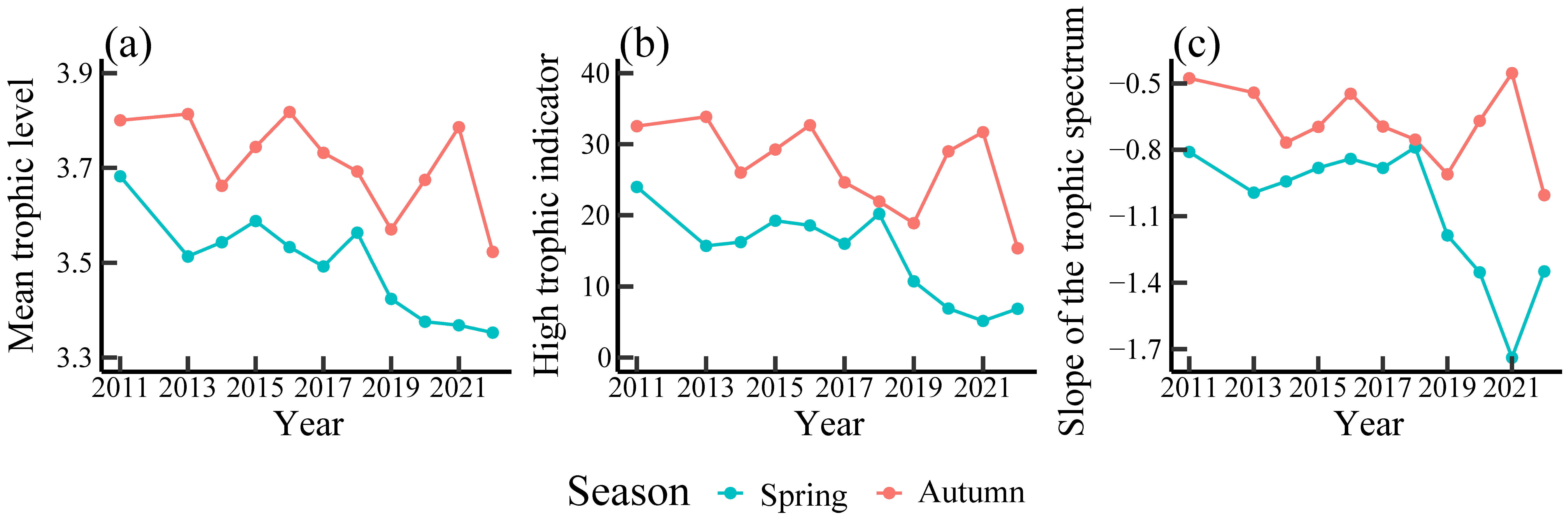
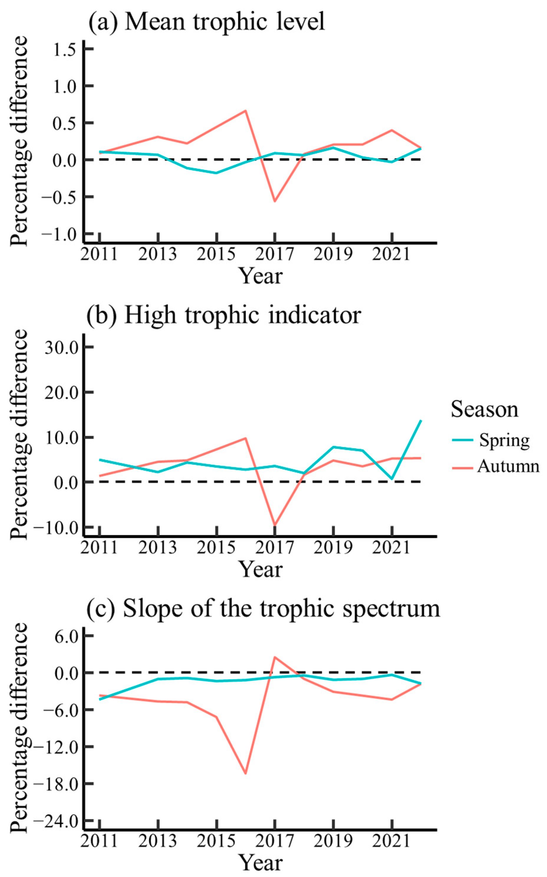
3.3. Temporal Variations in Trophic Indicators

In scenario B, three indicators showed great temporal variations, with fluctuations observed in both spring and autumn (Figure 7). Fish communities in autumn showed higher trophic levels and indicator values than those in spring.

All three indicators showed decreasing trends during these years. The MTL of the fish community in Haizhou Bay had a significant downtrend in the spring of 2011 and 2013–2022 (Mann-Kendall Z = −2.96, p < 0.01;

Table 3. Variations in the mean trophic level, high trophic indicator, and slope of the trophic spectrum of fish communities in Haizhou Bay.

Indicator	Seasons	Mann–Kendall Test		Sen’s Slope
		Z	p-Value
Mean trophic level	Spring	−2.96	0.00 *	−0.03
	Autumn	−1.71	0.09	−0.02
High trophic indicator	Spring	−2.34	0.02 *	−1.60
	Autumn	−1.87	0.06 +	−1.33
Slope of the trophic spectrum	Spring	−1.71	0.09	−0.05
	Autumn	−1.09	0.28	−0.03

Note: * means difference is significant (p < 0.05) and ⁺ means difference is marginally significant (p = 0.06).

). Sen’s slope indicated the annual decline of 0.03 trophic levels. In autumn, the variation in MTL was not significant (Mann–Kendall Z = −1.71, p = 0.09; Table 3). HTI showed a significant decline in spring (Mann–Kendall Z = −2.34, p = 0.02; Table 3) and marginally significant decline in autumn (Mann–Kendall Z = −1.87, p = 0.06; Table 3), with annual decreases of 1.60 and 1.33 based on Sen’s estimator of the slope, respectively. The decrease in the slope was not significant (Mann–Kendall p > 0.05; Table 3) in both spring and autumn.

Three indicators showed different responses between scenarios A and B (Figure 8). MTL was almost the same between the two scenarios, with percentage difference being less than 1.00%. Conversely, the percentage difference of HTI ranged from −9.56% to 13.78%, which showed high sensitivity to the division of the trophic functional group based on size structure. The percentage difference of the slope fluctuated between spring and autumn, with ranges of [−4.37%, −0.30%] and [−16.38%, 2.49%], respectively. In most cases, the slope values in scenario B were lower than those in scenario A, especially during the autumn of 2016.

4. Discussion

4.1. Stable Isotopic Values and Trophic Levels

According to Amundsen [51], the trophic niche of fish is composed of the between-phenotype component and within-phenotype component. The between-phenotype component of the trophic niche indicates that dietary composition varies among individuals in different groups of the same species, which should be considered during the classification of functional groups. In this study, the heterogeneity of dietary variation during ontogeny was shown in scenario B, which reflects different trophic niches occupied by individuals with different sizes. The six species with distinct ontogenetic dietary shifts showed diverse functional traits, such as feeding habits, mouth position, and relative mouth size [24], which made it hard to find a fixed interval to distinguish the difference of diets. Moreover, optimal foraging theory [52] indicated that the predators would turn to foraging larger prey once predatory ability was sufficient and diet would abruptly shift. Therefore, the equidistant size classes were not appropriate to investigate the effects of ontogenetic dietary shifts and thresholds of size for ontogenetic dietary shifts should be considered in the classification of functional groups.

The results of stable isotopic analysis were affected by dietary composition and metabolic processes of fish [53]. Fish size not only determined the size range of prey [54], but also was one of the key factors affecting their metabolism [55]. Both of them indicated that the fish size of specimens played a key role in variation in stable isotope values. The nitrogen isotope values of predators were enriched by trophic fractionation [37], resulting in the crucial effects on isotope values due to the abundance and quality of prey. Anthropogenic nitrogen inputs from land might be one of the important factors affecting the isotopic values of fishes [56], which may result in the higher δ¹⁵N in the studies of adjacent waters [57,58], and indicated the importance of considering offshore distance when stable isotope analysis was conducted. Moreover, long-lived sedentary primary consumers were confirmed to be the appropriate baseline species that can control the variation in δ¹⁵N at the base of the food web [59], and A. farreri, a species of bivalve, was used in this study, while zooplankton was employed in studies of adjacent waters [57,58]. The discrepancy in baseline species may be one of the reasons for the difference in trophic levels.

Both stomach content analysis and stable isotope analysis are confirmed to reliably discriminate the trophic level of fish [59,60]. However, stable isotope analysis provides long-term information about trophic levels, while stomach content analysis gives a snapshot of trophic levels [59], which explains the difference in trophic levels between the two methods. Environmental factors, such as sea bottom temperature and salinity, are key factors influencing the distribution of potential prey (e.g., Zhao et al. [61] and Luan et al. [62]). Thus, when trophic levels from different methods are compared, it is necessary to investigate environmental and biological factors (e.g., distribution of prey), of which the stability may be one of the conditions that keep trophic levels calculated from the two methods consistent. Moreover, the meta-analytical approaches could integrate samples from conditions with different factors and may be unreliable under specific conditions.

4.2. Effect of Ontogenetic Dietary Shifts on the Trophic Spectrum

In this study, the variations in the trophic level of fish during ontogenetic dietary shifts varied greatly among species, which will have great impacts on trophic structure. Top–down control is one of the vital effects of high-trophic-level organisms [63], which is affected by the biomass [64] and disturbance of predators [65]. For fish species with distinct ontogenetic dietary shifts, the trophic levels of small individuals are usually lower than those of large individuals and the role of species as predators is mainly reflected by the latter. Thus, it is necessary to identify functional groups that play a key role in the top–down control and further accurately quantify the intensity of this control. In scenarios that consider size structure (i.e., scenario B), different trophic levels are assigned to individuals within each size class and the intensity of top–down control is dispersed to different prey and reduces the foraging mortality of them, which will reshape the trophic relationship and reduce the risk of collapse of prey population in most cases.

Prior studies have suggested that understanding trophic relationships is a critical component in the development of harvest [66,67,68], with biomass per trophic level serving as a fundamental basis for formulation of catch [44,69]. Our study showed that in scenario A, a higher biomass was estimated between trophic level 3.4 and 3.8, which could lead to a higher exploitation rate at these trophic levels than expected in the practice of output control, intensively altering the trophic structure of fish communities and triggering ecosystem collapse. Notably, individuals of mid-trophic-level species play important roles in linking primary and secondary consumers with apex predators [70].

According to Galván [17], about 40% of 131 marine fishes displayed significant relationships between their size and trophic position, highlighting the need to understand discrepant feeding habits within species. Moreover, species with distinct ontogenetic dietary shifts can be the dominant species at specific trophic levels, and understanding the effects of ontogenetic dietary shifts is of great significance for studies of trophic structure. However, functional group classification is mainly based on taxonomy, which may mask differences within species and partially neglects the change of trophic structure [71]. As an accessible biological parameter, size should be one basis of functional group division to better understand the trophic characteristic of fish species. Given that dominant species have been divided as an independent trophic functional group (e.g., Srithong et al. [72]), taking size as one of the bases during the functional group division should be promoted.

4.3. Effect of Ontogenetic Dietary Shifts on Trophic Indicators

In this study, we revealed discrepancies in the sensitivities of the three indicators to ontogenetic dietary shifts. Among these indicators, MTL and HTI showed similar trends when assessing the status of marine ecosystems [73] and predicting the impact of climate change [74], and MTL was found to be more suitable for application in communities with short food chains [43], both of which indicated that HTI can be replaced by MTL. However, HTI showed high sensitivity to fishing [43], making it a more appropriate indicator to reflect the effect of ontogeny on trophic structure. Conversely, MTL showed the lowest sensitivity, and the sensitivity of the slope to ontogenetic dietary shifts varied greatly with the structure of fish communities. Thus, the indicator of HTI should be prioritized in investigations of trophic relationships.

All the indicators tend to describe a fish community with better conditions (i.e., flatter slope and higher MTL and HTI) in the majority of cases where the size structure is considered, highlighting the positive effects of ontogenetic dietary shifts on fish communities. In a trophic spectrum, fish communities can be described as biomass distribution along trophic levels [15], and a healthier fish community can be interpreted as an optimized allocation of biomass across trophic levels. Different life stages (i.e., before and after dietary shift) induced predators with different sizes to target prey from diverse trophic levels, which was reflected in the distribution of the biomass of species in a wider range of trophic levels in scenario B, especially in spring. Such diversified predation pressure may help distribute biomass in different trophic levels and reduce the risk of rapid depletion of specific trophic levels [75]. However, the effects of ontogenetic dietary shifts are complex and vary across food webs [76,77]. According to the optimal foraging theory [52], a key driver of ontogenetic dietary shifts for individuals is to maximize energy supplement. Under conditions of limited prey availability, the demand of energy capture and limitation of new prey resources [77] may compel fish to prioritize foraging on high-energy-density prey. Such an intensified focus can exacerbate the depletion of these prey and partly explain the destabilizing aspect of an ontogenetic dietary shift.

How ontogenetic dietary shifts affect the ecosystem processes is complex and has dual-edged effects [77]. Different conditions of fish communities throughout years suggested that the effect of ontogenetic dietary shifts was determined not only by feeding habits [77], but also by the trophic interactions between predators and prey, which can be influenced by prey-predator assemblages [78]. Moreover, the proportion of biomass of the six species with distinct ontogenetic dietary shifts showed different roles that these species played in the fish community. Among them, S. elongata showed its vital effects on high trophic levels (trophic level > 4.0), while C. spinosus, L. polyactis and H. otakii played important roles in trophic levels between 3.5 and 4.5. This indicated that the effects of ontogenetic dietary shifts, whereby it is difficult to have a fixed pattern, varied greatly among species. Thus, we suggest that the effect of ontogenetic dietary shifts should be discussed in the specific context of species compositions, where the abundance of prey and predator matching in the same spatiotemporal environment is the key to affecting community dynamics.

4.4. Implications for Fishery Management

Although size-based methods [79], reference points [80] and indicators [81] are important tools in the assessment of fish populations, few of them consider the effects of an ontogenetic dietary shift. In fisheries, large individuals are often targeted to maximize economic values. Among the six species with distinct ontogenetic dietary shifts, five species showed increased trophic level during ontogeny, which indicated that the role of an apex predator was primarily implemented by larger individuals. Fishing can lead to an increase in unexploitable low-trophic-level species [44], and top–down control exerted by predators plays an important role in regulating the biomass of these species. Therefore, specific measures should be developed to maintain the biomass of large individuals to control unexploitable species. For example, the use of gillnets designed to target fish with a certain size range [82] can be promoted as a viable management strategy. Moreover, size-based fishery management measures mainly focused on small fish (e.g., minimum mesh size of gears and proportion limit of undersized fish in catch [83]). These measures help protect the stock of juvenile fish, but might make the large individuals that play the role of top predators suffer from higher fishing pressure, which would have negative impacts on the stability of the fish community. Thus, we recommend that specific quotas of different developmental stages should be allocated, respectively, to manage the resource efficiently.

Stock enhancement programs have been implemented in many countries [84]. Ecological carrying capacity is a key metric to determine the optimal number of target species for release, which is typically calculated by trophodynamic models (e.g., Wang et al. [85]). H. otakii is a prominent target species in stock enhancement, exhibiting different trophic levels across different life stages in this study. However, current studies often rely on mean trophic level of the species to investigate ecological carrying capacity [85], and released individuals are predominantly juveniles [86,87], which would cause the shortage of prey when a large number of juveniles are released and increase their mortality. Thus, studies focusing on detailed feeding habits across all developmental stages of target species are highly recommended.

In this study, although 206 specimens were used for stable isotope analysis, the range of specimen lengths still has the potential for expansion. Data limitations are a common challenge in fisheries assessment and management [88], and sufficient size-data may not be available in many surveys [17], both of which will limit the applications of dividing trophic functional groups by size. Moreover, a large number of samples with different size classes is needed to explore the trophic level comprehensively, which requires increased survey efforts and sufficient samples. In cases where data collection is restricted, we suggest that dominant fish species should be divided into different functional groups based on the size thresholds of diet shifts, which will help to explain the effect of ontogeny on trophic structure and better delineate the role of ontogeny, as well as make it feasible to collect such data in the fishery-dependent projects such as logbook collection of commercial fishing.

Haizhou Bay has suffered an obvious decline in species diversity [89] and an increase in the proportion of small-sized fish species [90]. Decreased MTL and HTI indicate that fishing has disturbed the fish community. Both size [91] and trophic level [3] of fish have decreased as a result of fishing, which reduces the variety of prey selection and therefore weakens the influence of size on trophic structures [77]. In addition, minimizing risk to fishery resources is one of the objectives of fishery management [92]. To achieve this, it is essential to mitigate fishing impact on ecosystems [93]. Future research should focus on undisturbed ecosystems with more complex trophic structures, where ontogenetic dietary shifts play a more pronounced role in trophic structure. Thus, we suggest that size structure should be explicitly considered when analyzing the trophic structure, and that indicators related to size composition should be incorporated into ecosystem assessments and management frameworks.

4.5. Limitations and Prospects

Invertebrates are crucial components in the food web of Haizhou Bay [94], serving not only as generalist feeders [95], but also as key prey species [96]. Moreover, predatory invertebrates can feed on other predators depending on body size [97], which complicates the effect of invertebrates on trophic structure. In this study, we only focused on fish species, and invertebrate species with complex trophic interactions were not analyzed. Thus, invertebrate species with distinct ontogenetic dietary shifts should also be classified into different functional groups when trophic structure of marine ecosystems are investigated.

Spatiotemporal heterogeneities of environmental factors, such as depth, salinity and sediment, have been observed in Haizhou Bay [21]. Meanwhile, the taxonomic diversity of fish communities [89] and feeding habits (e.g., Xu et al. [28]) of fish in Haizhou Bay were distinct among seasons, which made it necessary to investigate trophic structure under different spatial and seasonal scenarios. In our study, only fish communities in spring and autumn were analyzed, and spatial variations were omitted, which may partly mask the effects of ontogenetic dietary shifts and limit the generality of our conclusions.

In this study, both stomach content analysis and stable isotope analysis were used to determine the trophic levels of fish species. Although we chose the literature about Haizhou Bay or its adjacent area to reduce the variations of environmental and biological factors, the difference in trophic levels calculated by the two methods remained. In the future, we will pay more attention to monitoring the dynamic change in the size structure of communities of invertebrate and more vertebrate species, and explore the relationship between ontogeny and trophic position. In addition, a broader range of trophodynamic indicators should be applied to evaluate the sensitivity of the ontogeny of fish to support the implementation of ecosystem-based fishery management.

5. Conclusions

The size thresholds of ontogenetic dietary shifts should be considered in functional group classification. Therefore, we recommend detailed feeding habits before and after the size threshold of ontogenetic dietary shifts be investigated in ecosystem assessments and management frameworks. Ontogenetic dietary shifts can redistribute biomass across trophic levels, which is affected by community composition and may have positive and negative effects on the stability of trophic structure compared with communities without ontogenetic dietary shifts. Additionally, indicators with high sensitivity to ontogenetic dietary shifts are required in such studies, and fishery management measures should be optimized to balance the fishing pressure among fish of different life stages. Moreover, to comprehensively understand the effects of ontogenetic dietary shifts on trophic structure, the roles of predatory invertebrates need to be thoroughly investigated within the broader marine ecosystem context.

References

1. Tang, Q. Strategies of Research on Marine Food Web and Trophodynamics between High Trophic Levels. Mar. Fish. Res. 1999, 20, 1–6. [Google Scholar]
2. Libralato, S.; Pranovi, F.; Stergiou, K.; Link, J. Trophodynamics in Marine Ecology: 70 Years after Lindeman. Mar. Ecol. Prog. Ser. 2014, 512, 1–7. [Google Scholar] [CrossRef]
3. Agnetta, D.; Badalamenti, F.; Sweeting, C.J.; D’Anna, G.; Libralato, S.; Pipitone, C. Erosion of Fish Trophic Position: An Indirect Effect of Fishing on Food Webs Elucidated by Stable Isotopes. Phil. Trans. R. Soc. B 2024, 379, 20230167. [Google Scholar] [CrossRef] [PubMed]
4. Durante, L.M.; Beentjes, M.P.; Wing, S.R. Shifting Trophic Architecture of Marine Fisheries in New Zealand: Implications for Guiding Effective Ecosystem-based Management. Fish Fish. 2020, 21, 813–830. [Google Scholar] [CrossRef]
5. Rombouts, I.; Beaugrand, G.; Fizzala, X.; Gaill, F.; Greenstreet, S.P.R.; Lamare, S.; Le Loc’h, F.; McQuatters-Gollop, A.; Mialet, B.; Niquil, N.; et al. Food Web Indicators under the Marine Strategy Framework Directive: From Complexity to Simplicity? Ecol. Indic. 2013, 29, 246–254. [Google Scholar] [CrossRef]
6. Keramidas, I.; Dimarchopoulou, D.; Ofir, E.; Scotti, M.; Tsikliras, A.C.; Gal, G. Ecotrophic Perspective in Fisheries Management: A Review of Ecopath with Ecosim Models in European Marine Ecosystems. Front. Mar. Sci. 2023, 10, 1182921. [Google Scholar] [CrossRef]
7. Arreguín-Sánchez, F. Holistic Approach to Ecosystem-Based Fisheries Management: Linking Biological Hierarchies for Sustainable Fishing; Springer International Publishing: Cham, Switzerland, 2022; ISBN 978-3-030-96846-5. [Google Scholar]
8. Berdnikov, S.V.; Selyutin, V.V.; Surkov, F.A.; Tyutyunov, Y.V. Modeling of Marine Ecosystems: Experience, Modern Approaches, Directions of Development (Review). Part 2. Population and Trophodynamic Models. Phys. Oceanogr. 2022, 38, 182–203. [Google Scholar]
9. Crowder, L.B.; Hazen, E.L.; Avissar, N.; Bjorkland, R.; Latanich, C.; Ogburn, M.B. The Impacts of Fisheries on Marine Ecosystems and the Transition to Ecosystem-Based Management. Annu. Rev. Ecol. Evol. Syst. 2008, 39, 259–278. [Google Scholar] [CrossRef]
10. Steele, J.H. The Structure of Marine Ecosystems; Harvard University Press: Cambridge, MA, USA, 1974; ISBN 978-0-674-36746-3. [Google Scholar]
11. Polovina, J.J. Model of a Coral Reef Ecosystem: I. The ECOPATH Model and Its Application to French Frigate Shoals. Coral Reefs 1984, 3, 1–11. [Google Scholar] [CrossRef]
12. Wang, C.; Jiang, Z.; Zhou, L.; Dai, B.; Song, Z. A Functional Group Approach Reveals Important Fish Recruitments Driven by Flood Pulses in Floodplain Ecosystem. Ecol. Indic. 2019, 99, 130–139. [Google Scholar] [CrossRef]
13. Vanalderweireldt, L.; Albouy, C.; Le Loc’h, F.; Millot, R.; Blestel, C.; Patrissi, M.; Marengo, M.; Garcia, J.; Bousquet, C.; Barrier, C.; et al. Ecosystem Modelling of the Eastern Corsican Coast (ECC): Case Study of One of the Least Trawled Shelves of the Mediterranean Sea. J. Mar. Syst. 2022, 235, 103798. [Google Scholar] [CrossRef]
14. Wanjari, R.N.; Shah, T.H.; Telvekar, P.; Bhat, F.A.; Abubakr, A.; Bhat, B.A.; Darve, S.I.; Ramteke, K.K.; Mathialagan, D.; Magloo, A.H.; et al. Assessing Ecosystem Health: A Preliminary Investigation of the Gosikhurd Dam Ecosystem Structure and Functioning, an Appraisal Based on Ecological Modelling, India. Environ. Monit. Assess. 2024, 196, 815. [Google Scholar] [CrossRef] [PubMed]
15. Gascuel, D.; Bozec, Y.-M.; Chassot, E.; Colomb, A.; Laurans, M. The Trophic Spectrum: Theory and Application as an Ecosystem Indicator. ICES J. Mar. Sci. 2005, 62, 443–452. [Google Scholar] [CrossRef]
16. Woodland, R.J.; Secor, D.H. Benthic-pelagic Coupling in a Temperate Inner Continental Shelf Fish Assemblage. Limnol. Oceanogr. 2013, 58, 966–976. [Google Scholar] [CrossRef]
17. Galván, D.; Sweeting, C.; Reid, W. Power of Stable Isotope Techniques to Detect Size-Based Feeding in Marine Fishes. Mar. Ecol. Prog. Ser. 2010, 407, 271–278. [Google Scholar] [CrossRef]
18. Colléter, M.; Gascuel, D.; Ecoutin, J.-M.; Tito De Morais, L. Modelling Trophic Flows in Ecosystems to Assess the Efficiency of Marine Protected Area (MPA), a Case Study on the Coast of Sénégal. Ecol. Model. 2012, 232, 1–13. [Google Scholar] [CrossRef]
19. Du Pontavice, H.; Gascuel, D.; Reygondeau, G.; Stock, C.; Cheung, W.W.L. Climate-induced Decrease in Biomass Flow in Marine Food Webs May Severely Affect Predators and Ecosystem Production. Glob. Chang. Biol. 2021, 27, 2608–2622. [Google Scholar] [CrossRef]
20. Thiaw, M.; Gascuel, D.; Sadio, O.; Ndour, I.; Diadhiou, H.D.; Kantoussan, J.; Faye, S.; Thiam, M.; Meissa, B.; Brehmer, P. Efficiency of Two Contrasted Marine Protected Areas (MPA) in West Africa over a Decade of Fishing Closure. Ocean Coast. Manag. 2021, 210, 105655. [Google Scholar] [CrossRef]
21. Ren, Y. (Ed.) Fishery Resources and Habitat Environment in Haizhou Bay; China Agriculture Press: Beijing, China, 2022; ISBN 978-7-109-29397-7. [Google Scholar]
22. Chen, X. (Ed.) Fisheries Resources and Fishery Oceangraphy; Marine Press: Beijing, China, 2004; ISBN 7-5027-6118-7. [Google Scholar]
23. Yin, J.; Xue, Y.; Li, Y.; Zhang, C.; Xu, B.; Liu, Y.; Ren, Y.; Chen, Y. Evaluating the Efficacy of Fisheries Management Strategies in China for Achieving Multiple Objectives under Climate Change. Ocean Coast. Manag. 2023, 245, 106870. [Google Scholar] [CrossRef]
24. Zhang, X.; Wang, J.; Xu, B.; Zhang, C.; Xue, Y.; Ren, Y. Spatio-temporal variations of functional diversity of fish communities in Haizhou Bay. Chin. J. Appl. Ecol. 2019, 30, 3233–3244. [Google Scholar]
25. Wu, X.; Ding, X.; Jiang, X.; Xu, B.; Zhang, C.; Ren, Y.; Xue, Y. Variations in the Mean Trophic Level and Large Fish Index of Fish Community in Haizhou Bay, China. Chin. J. Appl. Ecol. 2019, 30, 2829–2836. [Google Scholar]
26. Xu, B.; Ren, Y.; Chen, Y.; Xue, Y.; Zhang, C.; Wan, R. Optimization of Stratification Scheme for a Fishery-Independent Survey with Multiple Objectives. Acta Oceanol. Sin. 2015, 34, 154–169. [Google Scholar] [CrossRef]
27. Jin, X.; Zhao, X.; Meng, T.; Cui, Y. The Yellow Sea and Bohai Sea Biological Resources and Habitats; Science Press: Beijing, China, 2005; ISBN 978-7-03-015476-7. [Google Scholar]
28. Xu, L.; Xue, Y.; Xu, B.; Ren, Y.; Dou, S. Feeding Ecology of Hexagrammos otakii in Haizhou Bay. J. Fish. Sci. China 2018, 25, 608. [Google Scholar] [CrossRef]
29. Chen, W.; Ren, X.; Xu, B.; Zhang, C.; Ren, Y.; Xue, Y. Understanding the Feeding Ecology of Cynoglossus joyneri in Haizhou Bay Based on Stable Isotope Analysis. Chin. J. Appl. Ecol. 2021, 32, 1080–1086. [Google Scholar]
30. Liu, X. Study on Feeding Ecology and Food Relations of Two High Trophic Level Fishes in Haizhou Bay. Master’s Thesis, Ocean University of China, Qingdao, China, 2015. [Google Scholar]
31. Wang, R.; Zhang, C.; Xu, B.; Ren, Y.; Xue, Y. Feeding Strategy and Prey Selectivity of Chelidonichthys spinosus during Autumn in Haizhou Bay. J. Fish. Sci. China 2018, 25, 1059–1070. [Google Scholar] [CrossRef]
32. Xue, Y.; Jin, X.; Zhang, B.; Liang, Z. Seasonal, Diel and Ontogenetic Variation in Feeding Patterns of Small Yellow Croaker in the Central Yellow Sea. J. Fish Biol. 2005, 67, 33–50. [Google Scholar] [CrossRef]
33. He, Z.; Zhang, Y.; Xue, L.; Jin, H.; Zhou, Y. Seasonal and Ontogenetic Diet Composition Variation of Collichthys lucidus in Inshore Waters in the North of East China Sea. Mar. Fish. 2012, 34, 270–276. [Google Scholar]
34. Zhang, B.; Tang, Q. Study on Trophic Level of Important Resources Species at High Trophic Levels in the Bohai Sea, Yellow Sea and East China. Adv. Mar. Sci. 2004, 22, 393–404. [Google Scholar]
35. Bai, H.; Wang, Y.; Zhang, T.; Huang, L.; Sun, Y. Trophic Levels and Feeding Characters of Marine Fishes in the Yellow Sea and Northern East China Sea Based on Stable Isotope Analysis. Prog. Fish. Sci. 2021, 42, 10–17. [Google Scholar] [CrossRef]
36. Ren, X.; Liu, Y.; Xu, B.; Zhang, C.; Ren, Y.; Cheng, Y.; Xue, Y. Ecosystem Structure in the Haizhou Bay and Adjacent Waters Based on Ecopath Model. Haiyang Xuebao 2020, 42, 101–109. [Google Scholar]
37. Post, D.M. Using Stable Isotopes to Estimate Trophic Position: Models, Methods, and Assumptions. Ecology 2002, 83, 703–718. [Google Scholar] [CrossRef]
38. Guitton, J.; Colleter, M.; Gatti, P.; Gascuel, D. EcoTroph: An Implementation of the EcoTroph Ecosystem Modelling Approach. 2022. R Package Version 1.6.1. Available online: https://CRAN.R-project.org/package=EcoTroph (accessed on 12 May 2025).
39. R Core Team. R: A Language and Environment for Statistical Computing; R Foundation for Statistical Computing: Vienna, Austria, 2023. [Google Scholar]
40. Wickham, H. Ggplot2: Elegant Graphics for Data Analysis, 2nd ed.; Use R! Springer International Publishing: Cham, Switzerland, 2016; ISBN 978-3-319-24277-4. [Google Scholar]
41. Shin, Y.-J.; Shannon, L.J. Using Indicators for Evaluating, Comparing, and Communicating the Ecological Status of Exploited Marine Ecosystems. 1. The IndiSeas Project. ICES J. Mar. Sci. 2010, 67, 686–691. [Google Scholar] [CrossRef]
42. Su, L.; Chen, Z.; Zhang, K.; Xu, Y.; Xu, S.; Wang, K. Decadal-Scale Variation in Mean Trophic Level in Beibu Gulf Based on Bottom-Trawl Survey Data. Mar. Coast. Fish. 2021, 13, 174–182. [Google Scholar] [CrossRef]
43. Bourdaud, P.; Gascuel, D.; Bentorcha, A.; Brind’Amour, A. New Trophic Indicators and Target Values for an Ecosystem-Based Management of Fisheries. Ecol. Indic. 2016, 61, 588–601. [Google Scholar] [CrossRef]
44. Rehren, J.; Gascuel, D. Fishing Without a Trace? Assessing the Balanced Harvest Approach Using EcoTroph. Front. Mar. Sci. 2020, 7, 510. [Google Scholar] [CrossRef]
45. Rooney, N.; McCann, K.; Gellner, G.; Moore, J.C. Structural Asymmetry and the Stability of Diverse Food Webs. Nature 2006, 442, 265–269. [Google Scholar] [CrossRef] [PubMed]
46. Lindeman, R.L. The Trophic-Dynamic Aspect of Ecology. Ecology 1942, 23, 399–417. [Google Scholar] [CrossRef]
47. Mann, H.B. Nonparametric Tests Against Trend. Econometrica 1945, 13, 245. [Google Scholar] [CrossRef]
48. Kendall, M.G. Rank Correlation Methods; Charles Griffin: London, UK, 1975. [Google Scholar]
49. Kale, S. Trend Analysis and Future Forecasting of Marine Capture Fisheries Production of Turkey. Res. Mar. Sci. 2020, 5, 773–794. [Google Scholar]
50. Sen, P.K. Estimates of the Regression Coefficient Based on Kendall’s Tau. J. Am. Stat. Assoc. 1968, 63, 1379–1389. [Google Scholar] [CrossRef]
51. Amundsen, P.-A.; Gabler, H.-M.; Staldvik, F.J. A New Approach to Graphical Analysis of Feeding Strategy from Stomach Contents Data—Modification of the Costello (1990) Method. J. Fish Biol. 1996, 48, 607–614. [Google Scholar] [CrossRef]
52. Gerking, S.D. Feeding Ecology of Fish; Academic Press: San Diego, CA, USA, 1994; ISBN 978-0-12-280780-0. [Google Scholar]
53. Tian, J.; Li, J.; Dong, H.; Zeng, X.; Zhang, J. Application of Stable Isotope Technology in Feeding Habit Research of Aquatic Animals. Chin. J. Fish. 2023, 36, 131–137. [Google Scholar]
54. Mittelbach, G.G.; Persson, L. The Ontogeny of Piscivory and Its Ecological Consequences. Can. J. Fish. Aquat. Sci. 1998, 55, 1454–1465. [Google Scholar] [CrossRef]
55. Pecquerie, L.; Nisbet, R.M.; Fablet, R.; Lorrain, A.; Kooijman, S.A.L.M. The Impact of Metabolism on Stable Isotope Dynamics: A Theoretical Framework. Phil. Trans. R. Soc. B 2010, 365, 3455–3468. [Google Scholar] [CrossRef]
56. Nixon, S.W.; Buckley, B.A.; Granger, S.L.; Entsua-Mensah, M.; Ansa-Asare, O.; White, M.J.; McKinney, R.A.; Mensah, E. Anthropogenic Enrichment and Nutrients in Some Tropical Lagoons of Ghana, West Africa. Ecol. Appl. 2007, 17, S144–S164. [Google Scholar] [CrossRef]
57. Han, D.; Xue, Y.; Ren, Y.; Ma, Q. Spatial and Seasonal Variations in the Trophic Spectrum of Demersal Fish Assemblages in Jiaozhou Bay, China. Chin. J. Ocean. Limnol. 2015, 33, 934–944. [Google Scholar] [CrossRef]
58. Zhang, Y.; Dong, J.; Sun, X.; Zhan, Q.; Wang, L.; Zhang, X. Trophic Structure of Fishery Assemblage in Surrounding Waters of Lingshan Island Based on Stable Isotope Analysis. Period. Ocean Univ. China 2022, 52, 40–51. [Google Scholar]
59. Vander Zanden, M.J.; Cabana, G.; Rasmussen, J.B. Comparing Trophic Position of Freshwater Fish Calculated Using Stable Nitrogen Isotope Ratios (δ15 N) and Literature Dietary Data. Can. J. Fish. Aquat. Sci. 1997, 54, 1142–1158. [Google Scholar] [CrossRef]
60. Rybczynski, S.M.; Walters, D.M.; Fritz, K.M.; Johnson, B.R. Comparing Trophic Position of Stream Fishes Using Stable Isotope and Gut Contents Analyses. Ecol. Freshw. Fish 2008, 17, 199–206. [Google Scholar] [CrossRef]
61. Zhao, M.; Xu, Z. Abundance and Distribution of Shrimps in Different Seasons in the Southern Haizhou Bay of Jiangsu Province. Mar. Sci. Bull. 2012, 31, 38–44. [Google Scholar]
62. Luan, J.; Zhang, C.; Xu, B.; Xue, Y.; Ren, Y. Modelling the Spatial Distribution of Three Portunidae Crabs in Haizhou Bay, China. PLoS ONE 2018, 13, e0207457. [Google Scholar] [CrossRef] [PubMed]
63. Terborgh, J.; Lopez, L.; Nuñez, P.; Rao, M.; Shahabuddin, G.; Orihuela, G.; Riveros, M.; Ascanio, R.; Adler, G.H.; Lambert, T.D.; et al. Ecological Meltdown in Predator-Free Forest Fragments. Science 2001, 294, 1923–1926. [Google Scholar] [CrossRef] [PubMed]
64. Gasche, L.; Gascuel, D. EcoTroph: A Simple Model to Assess Fishery Interactions and Their Impacts on Ecosystems. ICES J. Mar. Sci. 2013, 70, 498–510. [Google Scholar] [CrossRef]
65. Baum, J.K.; Worm, B. Cascading Top-down Effects of Changing Oceanic Predator Abundances. J. Anim. Ecol. 2009, 78, 699–714. [Google Scholar] [CrossRef] [PubMed]
66. Kaplan, I.C.; Hansen, C.; Morzaria-Luna, H.N.; Girardin, R.; Marshall, K.N. Ecosystem-Based Harvest Control Rules for Norwegian and US Ecosystems. Front. Mar. Sci. 2020, 7, 652. [Google Scholar] [CrossRef]
67. Bellier, E.; Sæther, B.-E.; Engen, S. Sustainable Strategies for Harvesting Predators and Prey in a Fluctuating Environment. Ecol. Model. 2021, 440, 109350. [Google Scholar] [CrossRef]
68. Rossi, S.P.; Cox, S.P.; Hammill, M.O.; Den Heyer, C.E.; Swain, D.P.; Mosnier, A.; Benoît, H.P. Forecasting the Response of a Recovered Pinniped Population to Sustainable Harvest Strategies That Reduce Their Impact as Predators. ICES J. Mar. Sci. 2021, 78, 1804–1814. [Google Scholar] [CrossRef]
69. Garcia, S.M.; Rice, J.; Charles, A. Balanced Harvesting in Fisheries: A Preliminary Analysis of Management Implications. ICES J. Mar. Sci. 2016, 73, 1668–1678. [Google Scholar] [CrossRef]
70. Choy, C.; Wabnitz, C.; Weijerman, M.; Woodworth-Jefcoats, P.; Polovina, J. Finding the Way to the Top: How the Composition of Oceanic Mid-Trophic Micronekton Groups Determines Apex Predator Biomass in the Central North Pacific. Mar. Ecol. Prog. Ser. 2016, 549, 9–25. [Google Scholar] [CrossRef]
71. Liang, C.; Pauly, D. Fisheries Impacts on China’s Coastal Ecosystems: Unmasking a Pervasive ‘Fishing down’ Effect. PLoS ONE 2017, 12, e0173296. [Google Scholar] [CrossRef]
72. Srithong, N.; Jensen, K.R.; Jarernpornnipat, A. Application of the Ecopath Model for Evaluation of Ecological Structure and Function for Fisheries Management: A Case Study from Fisheries in Coastal Andaman Sea, Thailand. Reg. Stud. Mar. Sci. 2021, 47, 101972. [Google Scholar] [CrossRef]
73. Ju, P.; Cheung, W.W.L.; Chen, M.; Xian, W.; Yang, S.; Xiao, J. Comparing Marine Ecosystems of Laizhou and Haizhou Bays, China, Using Ecological Indicators Estimated from Food Web Models. J. Mar. Syst. 2020, 202, 103238. [Google Scholar] [CrossRef]
74. Moullec, F.; Barrier, N.; Drira, S.; Guilhaumon, F.; Marsaleix, P.; Somot, S.; Ulses, C.; Velez, L.; Shin, Y.-J. An End-to-End Model Reveals Losers and Winners in a Warming Mediterranean Sea. Front. Mar. Sci. 2019, 6, 345. [Google Scholar] [CrossRef]
75. Caskenette, A.L.; McCann, K.S. Biomass Reallocation between Juveniles and Adults Mediates Food Web Stability by Distributing Energy Away from Strong Interactions. PLoS ONE 2017, 12, e0170725. [Google Scholar] [CrossRef] [PubMed]
76. Nilsson, K.A.; McCann, K.S.; Caskenette, A.L. Interaction Strength and Stability in Stage-structured Food Web Modules. Oikos 2018, 127, 1494–1505. [Google Scholar] [CrossRef]
77. Sánchez-Hernández, J.; Nunn, A.D.; Adams, C.E.; Amundsen, P. Causes and Consequences of Ontogenetic Dietary Shifts: A Global Synthesis Using Fish Models. Biol. Rev. 2019, 94, 539–554. [Google Scholar] [CrossRef]
78. Gao, M.; Dong, X.; Zhang, C.; Xu, B.; Ji, Y.; Ren, Y.; Xue, Y. Influencing Factors of Predation on Five Keystone Prey Species in Haizhou Bay Based on Delta-GAMMs. Chin. J. Appl. Ecol. 2023, 34, 1137–1145. [Google Scholar]
79. Rudd, M.B.; Thorson, J.T. Accounting for Variable Recruitment and Fishing Mortality in Length-Based Stock Assessments for Data-Limited Fisheries. Can. J. Fish. Aquat. Sci. 2018, 75, 1019–1035. [Google Scholar] [CrossRef]
80. Froese, R.; Stern-Pirlot, A.; Winker, H.; Gascuel, D. Size Matters: How Single-Species Management Can Contribute to Ecosystem-Based Fisheries Management. Fish. Res. 2008, 92, 231–241. [Google Scholar] [CrossRef]
81. Miranda, L.E.; Funk, H.G.; Palmieri, M.; Stafford, J.D.; Nichols, M.E. Length in Assessing Status of Freshwater Fish Populations: A Review. N. Am. J. Fish. Manag. 2024, 44, 1092–1110. [Google Scholar] [CrossRef]
82. Zhan, B. (Ed.) Fishery Stock Assessment; China Agriculture Press: Beijing, China, 1995. [Google Scholar]
83. Cao, L.; Chen, Y.; Dong, S.; Hanson, A.; Huang, B.; Leadbitter, D.; Little, D.C.; Pikitch, E.K.; Qiu, Y.; Sadovy De Mitcheson, Y.; et al. Opportunity for Marine Fisheries Reform in China. Proc. Natl. Acad. Sci. USA 2017, 114, 435–442. [Google Scholar] [CrossRef] [PubMed]
84. Liao, I.; Su, M.S.; Leaño, E.M. Status of Research in Stock Enhancement and Sea Ranching. Rev. Fish Biol. Fish. 2003, 13, 151–163. [Google Scholar] [CrossRef]
85. Wang, Z.; Feng, J.; Lozano-Montes, H.M.; Loneragan, N.R.; Zhang, X.; Tian, T.; Wu, Z. Estimating Ecological Carrying Capacity for Stock Enhancement in Marine Ranching Ecosystems of Northern China. Front. Mar. Sci. 2022, 9, 936028. [Google Scholar] [CrossRef]
86. Kitada, S. Lessons from Japan Marine Stock Enhancement and Sea Ranching Programmes over 100 Years. Rev. Aquac. 2020, 12, 1944–1969. [Google Scholar] [CrossRef]
87. Yuan, J.; Lin, H.; Wu, L.; Zhuang, X.; Ma, J.; Kang, B.; Ding, S. Resource Status and Effect of Long-Term Stock Enhancement of Large Yellow Croaker in China. Front. Mar. Sci. 2021, 8, 743836. [Google Scholar] [CrossRef]
88. Costello, C.; Ovando, D.; Hilborn, R.; Gaines, S.D.; Deschenes, O.; Lester, S.E. Status and Solutions for the World’s Unassessed Fisheries. Science 2012, 338, 517–520. [Google Scholar] [CrossRef]
89. Su, W.; Xue, Y.; Ren, Y. Temporal and Spatial Variation in Taxonomic Diversity of Fish in Haizhou Bay: The Effect of Environmental Factors. J. Fish. Sci. China 2013, 20, 624–634. [Google Scholar]
90. Sui, H.; Xue, Y.; Ren, Y.; Zou, Y.; Yu, L. Studies on the Ecological Groups of Fish Communities in Haizhou Bay, China. Period. Ocean Univ. China 2017, 47, 59–71. [Google Scholar]
91. Sun, P.; Liang, Z.-L.; Yu, Y.; Tang, Y.-L.; Zhao, F.-F.; Huang, L.-Y. Trawl Selectivity-Induced Evolution Effects on Age Structure and Size-at-Age of Largehead Hairtail (Trichiurus Lepturus) Linnaeus, 1758 in the East China Sea, China. J. Appl. Ichthyol. 2015, 31, 657–664. [Google Scholar] [CrossRef]
92. Butterworth, D. Experiences in the Evaluation and Implementation of Management Procedures. ICES J. Mar. Sci. 1999, 56, 985–998. [Google Scholar] [CrossRef]
93. Zhou, S.; Smith, A.D.M.; Punt, A.E.; Richardson, A.J.; Gibbs, M.; Fulton, E.A.; Pascoe, S.; Bulman, C.; Bayliss, P.; Sainsbury, K. Ecosystem-Based Fisheries Management Requires a Change to the Selective Fishing Philosophy. Proc. Natl. Acad. Sci. USA 2010, 107, 9485–9489. [Google Scholar] [CrossRef] [PubMed]
94. Wu, J.; Liu, Y.; Sui, H.; Xu, B.; Zhang, C.; Ren, Y.; Xue, Y. Using Network Analysis to Identify Keystone Species in the Food Web of Haizhou Bay, China. Mar. Freshw. Res. 2020, 71, 469. [Google Scholar] [CrossRef]
95. Cheng, J.; Zhu, J.; Jiang, W. Study on the Feeding Habit and Trophic Level of Main Economic Invertebrates in the Huanghai Sea. Acta Oceanol. Sin. 1999, 18, 117–126. [Google Scholar]
96. Xu, C.; Xu, B.; Zhang, C.; Ren, Y.; Xue, Y. Identification of Keystone Prey Species in Haizhou Bay Food Web Based on SURF Index. Acta Ecol. Sin. 2019, 39, 9373–9378. [Google Scholar] [CrossRef]
97. Blanchard, J.L.; Jennings, S.; Law, R.; Castle, M.D.; McCloghrie, P.; Rochet, M.; Benoît, E. How Does Abundance Scale with Body Size in Coupled Size-structured Food Webs? J. Anim. Ecol. 2009, 78, 270–280. [Google Scholar] [CrossRef]
98. GB/T 35892-2018; Laboratory Animal−Guideline for the Ethical Review of Animal Welfare. General Administration of Quality Supervision, Inspection, and Quarantine of the People’s Republic of China, Standardization Administration of the People’s Republic of China: Beijing, China, 2018.
Figure 1. Sampling area in Haizhou Bay and adjacent waters, China, covering five sub-regions A–E. Spr.: spring, Aut.: autumn.
Fishes 10 00231 g001
Figure 2. Trophic levels for six fish species with distinct ontogenetic dietary shifts in Haizhou Bay in (a) scenario B and (b) scenario C. Dashed line shows the mean trophic level of the fish species (scenario A).
Fishes 10 00231 g002
Figure 3. Biomass trophic spectra of fish communities in Haizhou Bay during (a) spring and (b) autumn of 2011 and 2013–2022 in scenario B.
Fishes 10 00231 g003
Figure 4. Difference in the biomass trophic spectra of scenarios A (ETA, dashed line) and B (ETB, solid line) in Haizhou Bay during the (a) spring and (b) autumn of 2011 and 2013–2022. Note: differences are calculated as 100 × (ETBETA)/ETA, and 0 percentage difference showed biomass was not affected by ontogenetic dietary shifts.
Fishes 10 00231 g004
Figure 5. Stacked area chart of the proportion of biomass of the six species with distinct ontogenetic dietary shifts in scenario B (the upper half part of each plot) and A (the lower half part of each plot) in Haizhou Bay during the spring of 2011 and 2013–2022. Note: biomass (%) is calculated as 100 × (BijkBtotal jk), where Bijk is the biomass of species with distinct ontogenetic dietary shifts i at trophic level j in scenarios k, Btotal jk is the biomass of the whole fish community at trophic level j in scenario k.
Fishes 10 00231 g005
Figure 6. Stacked area chart of the proportion of biomass of the six species with distinct ontogenetic dietary shifts in scenarios B (the upper half part of each plot) and A (the lower half part of each plot) in Haizhou Bay during the autumn of 2011 and 2013–2022. Note: biomass (%) is calculated as 100 × (BijkBtotal jk), where Bijk is the biomass of species with distinct ontogenetic dietary shifts i at trophic level j in scenarios k, Btotal jk is the biomass of the whole fish community at trophic level j in scenario k.
Fishes 10 00231 g006
Figure 7. Temporal variations in (a) the mean trophic level, (b) high trophic indicator and (c) slope of the trophic spectrum of fish communities in Haizhou Bay during the spring and autumn of 2011 and 2013–2022 in scenario B.
Fishes 10 00231 g007
Figure 8. Difference in (a) the mean trophic level, (b) high trophic indicator, and (c) slope of the trophic spectrum among trophic spectra of scenarios A (ETA, dashed line) and B (ETB, solid line) in Haizhou Bay during the spring and autumn of 2011 and 2013–2022. Note: differences are calculated as 100 × (ETBETA)/ETA, and 0 percentage difference showed that the biomass was not affected by ontogenetic dietary shifts.
Fishes 10 00231 g008