Climate Risk in Intermediate Goods Trade: Impacts on China’s Fisheries Production

Abstract

Climate change, especially extreme weather events, has significantly heightened the vulnerability of fisheries production supply chains. This study firstly investigates the input-driven climate risks through intermediate goods trade and their indirect impacts on China’s fisheries sector and constructs the Climate Risk-Trade-Production Model (CRTPM). Key findings include: (1) The input-driven climate risk indicator for China’s fisheries sector has increased over the period 1995–2020, with Brazil, Canada, the United States, Japan, South Korea, and Russia as major contributors. (2) From 1995 to 2020, rising climate risk index in Brazil and Canada negatively affected China’s fisheries output, with a 1% increase in climate risk index resulting in production declines of 0.173% and 0.367%, respectively. (3) In contrast, a reduction in the climate risk index in the United States and Japan lowered intermediate goods prices, boosting China’s output by 0.934% and 0.172%, respectively, for every 1% decrease in the climate risk index. (4) Climate risk index in South Korea and Russia, while initially increasing, eventually stabilized, having minimal impact on China’s fisheries production. It is the importance of monitoring extreme weather events to mitigate the economic vulnerabilities of China’s fisheries.

1. Introduction

Climate change, especially the growing frequency of extreme weather events, has profoundly disrupted global supply chains, particularly in the fisheries sector [1,2,3]. Direct effects such as shifts in fish stock distribution, reduced marine productivity, and extreme events like heatwaves or cold surges [4,5], which destabilize fisheries output and increase economic vulnerability [6,7,8,9,10]. Indirectly, climate risks raise costs and limit access to essential inputs like fishmeal and fish oil, impacting aquaculture systems and global seafood supply [11,12,13,14,15,16]. These cascading disruptions reduce yields, elevate costs, and undermine food security, especially in regions heavily reliant on fisheries [17,18,19].

As a leading fisheries producer, China is heavily reliant on critical resources such as germplasm, fishmeal, fish oil, and advanced technical equipment, all of which are vulnerable to extreme weather events. Such events can drastically reduce aquatic biomass and deplete germplasm resources, leading to cascading effects on production. For example, marine heatwaves have been shown to significantly reduce kelp genetic diversity and alter population structures, affecting the survival rates of fish offspring [20]. Recurrent flooding also causes substantial mortality in freshwater fish populations, such as marble trout, which reduces genetic diversity and undermines efforts toward sustainable production [21]. Additionally, extreme weather negatively impacts the yields of soybean-based fish feed, a key input for aquaculture. Droughts and heatwaves in major soybean-producing nations like the United States and Brazil have reduced yields by 10–20%, driving up export prices and increasing production costs for importing countries like China [22,23]. These challenges are further compounded by the heightened demand for equipment maintenance due to disruptions caused by extreme weather. Coastal fisheries equipment manufacturers, for instance, often face increased pressure to adjust production schedules to meet fluctuating demand and repair damage from severe weather events [24]. As a result, extreme weather in regions supplying critical intermediate goods creates significant disruptions in China’s fisheries production, intensifying supply chain vulnerabilities and increasing economic pressures.

In summary, climate risk reduces primary production and increases production costs in fisheries, with these impacts propagating across borders through trade, thereby affecting supply chain efficiency and performance [25,26]. However, the existing literature has not sufficiently addressed the influence of climate risks on fisheries’ intermediate goods supply chains from a trade perspective. This study fills this gap by investigating the extent to which China’s fisheries production is impacted by climate risks in source countries supplying intermediate goods. The study’s marginal contributions are threefold: (1) it constructs a trade model for China’s fisheries production sector to theoretically explain how climate risks in source countries affect fisheries output; (2) it firstly proposes an input-driven climate risk indicator tailored to supply chains, quantifying these risks for China’s fisheries sector from 1995 to 2020; and (3) it empirically validates the indicator’s applicability and accuracy, demonstrating the measurable effects of source country climate risks on China’s fisheries output. By providing a novel perspective on the transmission of climate risks via intermediate goods trade, this study contributes to a deeper understanding of supply chain vulnerabilities in the context of global environmental change.

The remainder of this paper is structured as follows: Section 2 introduces the theoretical framework and methodology, detailing how climate risks in source countries impact China’s fisheries production and describing the construction of the input-driven climate risk indicator. Section 3 presents the results, offering an analysis of trends in the input-driven climate risk indicator alongside empirical findings. Finally, Section 4 provides a conclusion and discussion.

2. Method and Data

2.1. Data

This study covers the period from 1995 to 2020. Data on intermediate goods inputs (45 production sectors) for China’s fisheries production sector were sourced from the World Input-Output Table, which includes information from 78 countries and regions (Data Source: https://www.rug.nl/ggdc/valuechain/wiod). And the production data for China’s fisheries sector were obtained from the FAO statistics. While labor and capital input data were extracted from the China Fisheries Statistical Yearbook (1995–2021). In this analysis, the quantity of capital is represented by the year-end number of motor fishing vessels in China, following the methodology established by Tang et al. [27]. The technological progress in the fisheries sector was derived from the studies of Yang [28] and Zhang [29]. In this study, the technological progress was evaluated by first estimating total factor productivity (TFP) through the Cobb-Douglas production function. The derived TFP was then decomposed into technological progress and scale effects using Data envelopment analysis (DEA). Additionally, data on aquaculture area were sourced from the China Agricultural Statistical Yearbook (1995–2020). A detailed list of the specific variables and their corresponding names is provided in Appendix A.

The global climate risk index (CRI) was obtained from the study by Guo et al. [30], with the raw meteorological data sourced from the National Oceanic and Atmospheric Administration (NOAA). Figure 1 presents the trend of CRI for 78 countries and regions. According to the global input-output table, China’s fisheries production sector predominantly imports intermediate goods from countries such as the United States, Canada, Brazil, South Korea, Japan, and Russia. As illustrated in Figure 1 and Figure 2, CRI in Brazil and Canada has been on the rise, whereas that in the United States and Japan has been declining. CRI in Russia and South Korea has shown a slight increase, though the overall change is minimal and appears to be stabilizing. These six countries’ CRI data are used to validate the accuracy of the constructed Climate Risk-Trade-Production Model (CRTPM) in Section 2.2.

2.2. Theoretical Model

Building on a comprehensive literature review, this study posits that climate risk is transmitted through intermediate goods trade, thereby exerting an indirect influence on China’s fisheries production. To test this hypothesis, a production model incorporating intermediate goods trade and climate risk is developed, which is called the Climate Risk-Trade-Production Model (CRTPM), offering a theoretical framework to elucidate how climate risks in source countries impact fisheries production through trade channels.

Based on production theory, this model assumes that, with a constant level of output, the scale of production remains unchanged, and China’s fisheries sector operates under cost-minimization principles. The production process is modeled using a Constant Elasticity of Substitution (CES) production function, which is expressed as follows:

$$Q=A{({\alpha }_1{K}^{-\rho }+{\alpha }_2{L}^{-\rho }+{\alpha }_3{D}^{-\rho }+{\alpha }_4{Z}^{-\rho })}^{-{\displaystyle \frac{1}{\rho }}}$$

(1)

$$Q>0,K>0,L>0,D>0,Z>0$$

(2)

$$s.t:{\alpha }_1+{\alpha }_2+{\alpha }_3+{\alpha }_4=1$$

(3)

In Equation (1), Q represents the output of the fisheries production sector, while K, L, D, and Z denote the capital input, labor input, aquaculture area, and intermediate goods input, respectively. A signifies technological progress, and α represents the share of each input factor in the production process. Additionally, ρ reflects the elasticity of substitution, capturing the degree to which inputs can be substituted for one another within the production function.

Here, the intermediate goods input Z encompasses both domestically produced and imported goods. Following the Armington assumption of imperfect substitution, the substitution between these goods is modeled using a constant elasticity of substitution (CES) function.

$$Z={(\beta Z_d^{-\theta }+(1-\beta )Z_i^{-\theta })}^{-{\displaystyle \frac{1}{\theta }}}$$

(4)

$$\theta ={\displaystyle \frac{d{p}_d}{p_d}}\ast {\displaystyle \frac{P_i}{d{p}_i}}$$

(5)

$$s.t:0<\beta <1$$

(6)

In Equations (4)–(6), Z_d represents the input of domestically produced intermediate goods, while Z_i denotes the input of imported intermediate goods. The parameter θ reflects the elasticity of substitution, which is determined by the relative prices of domestic and imported goods. β indicates the proportion of domestic goods input, P_d is the price of domestic intermediate goods, and P_i is the price of imported intermediate goods.

Both domestic and imported intermediate goods prices are affected by climate risk. Increased climate risk typically results in a reduction in the demand for these goods, which in turn drives up their prices [31,32,33].

$$Z_d=f_d=f(P_d,CR{I}_d)$$

(7)

$$Z_i=f_i=f(P_i,CR{I}_i)$$

(8)

$$s.t:f_d>0,f_i>0$$

(9)

$$s.t:f_p^{\prime }<0,f_{CRI}^{\prime }<0$$

(10)

In Equations (7)–(10), CRI_d represents the domestic climate risk index, while CRI_i represents the climate risk index of intermediate goods source countries. The function f denotes the input function of intermediate goods, which follows the Armington assumption of imperfect substitutability and is therefore strictly greater than 0. The first derivative of f, denoted as f′, is negatively correlated with P and CRI, and is less than 0.

At a given production level, the cost function for China’s fisheries production sector is as follows.

$$C=P_{k}K+P_{l}L+P_{D}D+P_d{Z}_d+P_i{Z}_i$$

(11)

In Equation (11), C represents the production cost of the fisheries sector, while P_k, P_l, and P_D denote the prices of capital, labor, and aquaculture area, respectively. For the purpose of this study, these variables are treated as exogenous and standardized, with their values set to 1. Fixed price at 1 is a common normalization method used to simplify models, eliminate the arbitrariness of price levels, and more clearly analyze the effects of relative prices [34]. Based on the principle of cost minimization in production, the following equation is derived.

$$Z_d^{\prime }={\displaystyle \frac{P_i}{P_d}}{Z}_i^{\prime }$$

(12)

By combining Equations (1)–(12), we obtain:

$$(q-a){({\displaystyle \frac{Q}{A}})}^{\rho }={\displaystyle \frac{k}{K^{\rho }}}+{\displaystyle \frac{l}{L^{\rho }}}+{\displaystyle \frac{d}{D^{\rho }}}+{\displaystyle \frac{(\gamma dCR{I}_d+1)f_{i|CR{I}_i}^{\prime }dCR{I}_i+(\eta d{p}_d+1)f_{i|p_i}^{\prime }d{p}_i}{f_i^{2\theta +1}}}$$

(13)

$$q={\displaystyle \frac{dQ}{Q}},k={\displaystyle \frac{dK}{K}},l={\displaystyle \frac{dL}{L}},d={\displaystyle \frac{dD}{D}}$$

(14)

$$\gamma ={\alpha }_4\beta (\beta ({\displaystyle \frac{p_i}{p_d}}{)}^{-2\theta }+(1-\beta ))({\displaystyle \frac{p_i}{p_d}}{)}^{1-2(\theta +1)}>0$$

(15)

$$\eta ={\alpha }_4(1-\beta )(\beta ({\displaystyle \frac{p_i}{p_d}}{)}^{-2\theta }+(1-\beta ))({\displaystyle \frac{p_i}{p_d}}{)}^{1-2(\theta +1)}>0$$

(16)

Thus, based on Equation (13), the following scenarios can be drawn:

Scenario 1: Assuming that a, k, l, and d are constant, their values are set equal to zero. When dCRI_d > 0, dP_d > 0, dCRI_i > 0, dP_i > 0, f′_{i|CRI_i} < 0 and f′_{i|p_i} < 0, we have q < 0. This implies that the demand for intermediate goods is negatively correlated with both price and climate risk. As China’s climate risk increases, coupled with rising climate risks in the source countries of intermediate goods (Brazil and Canada), the prices of these goods tend to increase. Consequently, the cost of imports for China’s fisheries production sector rises, which leads to a reduction in output.

Scenario 2: Assuming that a, k, l, and d are constant, their values are set equal to zero. When dCRI_d > 0, dP_d > 0, dCRI_i < 0, dP_i < 0, f′_{i|CRI_i} < 0 and f′_{i|p_i} < 0, we have q > 0. This implies that the demand for intermediate goods is negatively correlated with both price and climate risk. When China’s climate risk increases, but the climate risk in the source countries of intermediate goods alleviates (Japan and the United States), the price of imported goods decreases. As a result, demand for imports rises, leading to reduced costs for China’s fisheries production sector and an increase in output.

Scenario 3: Assuming that a, k, l, and d are constant, their values are set equal to zero. When dCRI_d > 0, dP_d > 0, dCRI_i = 0, dP_i = 0, f′_{i|CRI_i} < 0, and f′_{i|p_i} < 0, we have q = 0. This implies that the demand for intermediate goods is negatively correlated with both price and climate risk. When China’s climate risk increases, but the climate risk in the source countries of intermediate goods remains unchanged (South Korea and Russia), the price of imported intermediate goods does not change. Consequently, there is no effect on the production costs or output of China’s fisheries sector.

2.3. Input-Driven Climate Risk Indicator of Intermediate Goods Supply Chain

To validate the above scenarios, we construct the Input-Driven Climate Risk Indicator in the section. This indicator is based on Wagner and Bode’s [35] definition of supply chain risk. We think that the definition of the indicator is that climate risk changes faced by intermediate goods supplier countries influence the output and price of these goods, thereby affecting production in the importing country. Drawing on supply chain risk models developed by Wagner and Bode [35], Su [36], and Zhu and Fang [37], the indicator integrates critical factors such as dependency on intermediate goods (Equation (17)), the concentration of intermediate goods suppliers (Equation (18)), and climate risk indices (Equation (19)).

The dependency on intermediate goods from a specific source country is defined as the ratio of imported intermediate goods from that country to the total intermediate goods input. A higher proportion indicates a greater reliance on that particular source country, which increases the vulnerability of the supply chain to disruptions originating from that country.

$$D_{ie}^f={\displaystyle \frac{{\displaystyle \sum _{c=1}^K{Z}_{ie}^{cf}}}{{\displaystyle \sum _{c=1}^K{Z}_{ee}^{cf}+{\displaystyle \sum _{i=1}^N{\displaystyle \sum _{c=1}^K{Z}_{ie}^{cf}}}}}}$$

(17)

$D_{ie}^f$ denotes the dependency of the fisheries production sector (f) in country (e) on imports of intermediate goods from source country (i). $Z_{ie}^{cf}$ represents the quantity of intermediate goods imported by the fisheries sector (f) in country (e) from source country (i). $Z_{ee}^{cf}$ represents the quantity of intermediate goods (c) supplied by country (e) itself and used in its fisheries sector (f).

The concentration of intermediate goods suppliers refers to the extent to which the source countries of intermediate goods are concentrated or dispersed. A higher concentration value indicates a greater reliance on a limited number of suppliers, thereby increasing the risk of supply chain disruptions. This study adopts the Herfindahl–Hirschman index (HHI) to construct a concentration indicator for intermediate goods suppliers, which measures the degree of concentration and its associated supply chain risks.

$$HH{I}_{ie}^f={\displaystyle \sum _i^N{\left(\frac{{\displaystyle \sum _{c=1}^K{Z}_{ie}^{cf}}}{{\displaystyle \sum _{i=1}^N{\displaystyle \sum _{c=1}^K{Z}_{ie}^{cf}}}}\right)}^2}$$

(18)

${HHI}_{ie}^f$ represents the concentration indicator for intermediate goods imported by the fisheries sector (f) in country (e) from source country (i). If the value of ${HHI}_{ie}^f$ is equal to 1, it indicates that all intermediate goods imported by country’s (e) fisheries sector (f) come from a single source country, implying a high dependency on that country. Conversely, if the value is 0, it means that country (e) does not import any intermediate goods from that particular source country and thus does not face any risk of supply chain disruption from that country.

This study adopts the climate risk index (CRI) construction method developed by Guo et al. [30] and applies the relevant data to build the climate risk index used in this analysis. The primary goal of this climate risk index is to capture the climate-related vulnerabilities faced by the source countries of intermediate goods, as these vulnerabilities may affect the supply chain and, in turn, the production of China’s fisheries sector.

For example, the extreme drought index (EDD) was calculated for each individual station. Records with missing values were excluded. The index was computed using the following formula:

$${\tau }_{i,n}={\displaystyle {\sum }_{t=1}^{365}{\tau }_{i,n,t}}$$

(19)

$${\tau }_{i,n,t}=\left\{\begin{array}{ll}1& if {\tau }_{i,n,t}\prec {\tau }_i^5\\ 0& if {\tau }_{i,n,t}\ge {\tau }_i^5\end{array}\right.$$

(20)

Here, τ_i⁵ is defined as the 5th percentile of historical daily humidity at station i, representing the threshold for extreme drought conditions. The value τ_i,n,t refers to the humidity at station i on day t of year n. If the daily humidity falls below the station-specific threshold, that day is classified as an extreme drought day. If the humidity is equal to or above the threshold, the day is not considered to be drought affected. Meanwhile, if τ are the lower 10th percentile of the historical daily average temperature of station, representing the threshold value for extreme low temperature (LTD); it is the 90th percentile of the historical daily average temperature of the station, representing the threshold value for extreme high temperatures (HTD); it is defined as the 95th percentile of the historical daily rainfall of station, representing the threshold value for extreme rainfall (ERD).

In the second step, after calculating the extreme drought index for each station, a regional extreme drought climate risk index was computed to represent the overall conditions across the country.

$${\tau }_n={\displaystyle \frac{1}{m}}{\displaystyle {\sum }_{i=1}^m{\tau }_{i,n}}$$

(21)

In the above equation, τ_n represents the average extreme drought climate risk index across all stations (m) in year n.

In the last step, we calculate the CRI.

$$\begin{array}{l}CR{I}_i=w_1{\overline{LTD}}_i+w_2{\overline{HTD}}_i+w_3\overline{ER{D}_i}+w_4{\overline{EDD}}_i\end{array}$$

(22)

LTD, HTD, ERD, and EDD represent the indices for extreme low temperature days, extreme high temperature days, extreme heavy rainfall days, and extreme drought days, respectively, for the intermediate goods source countries. Where W denotes the weight assigned to each extreme climate indicator in the overall climate risk index, W is set at 0.25 for each factor (the benchmark method adheres to the internationally recognized “Equal Weighting without Priori” principle on the Fifth Assessment Report (AR5) the Intergovernmental Panel on Climate Change (IPCC). Its theoretical foundation lies in that when the contributions of multiple indicators are uncertain, equal weight allocation can effectively prevent subjective bias while complying with the principle of minimum information loss by Rubinstein [38]. This methodology has been validated across 30 global climate risk assessments, demonstrating strong generalizability). The specific calculation method follows Guo et al. [30].

Thus, based on the dependency on intermediate goods source countries, the concentration of intermediate goods source countries, and the climate risk index of these source countries, we have constructed an input-driven climate risk indicator for the intermediate goods supply chain in China’s fisheries production sector.

$${CSC}_e^f=D_{ie}^f\times HH{I}_{ie}^f\times CR{I}_i$$

(23)

${CSC}_e^f$ represents the input-driven climate risk indicator from intermediate goods source country (i) to the fisheries production sector (f) in importing country (e). The larger this value, the greater the impact from climate risk faced by the source countries of intermediate goods.

To decompose the contribution of each indicator to the ${CSC}_e^f$ this study employs a two-stage averaging method to decompose the contribution of the $D_{ie}^f$, ${HHI}_{ie}^f$ and ${CRI}_i$ index. The specific decomposition formula is as follows:

$$\begin{array}{l}\Delta {CSC}_{ie}^f=D_{ie,t}^f\times HH{I}_{ie,t}^f\times CR{I}_{i,t}-D_{ie,t-1}^f\times HH{I}_{ie,t-1}^f\times CR{I}_{i,t-1}\\ ={\displaystyle \frac{1}{2}}(\Delta D_{ie,t}^f\times HH{I}_{ie,t}^f\times CR{I}_{i,t}+\Delta D_{ie,t}^f\times HH{I}_{ie,t-1}^f\times CR{I}_{i,t-1})\\ (Contribution of D_{ie}^f)\\ +{\displaystyle \frac{1}{2}}(D_{ie,t}^f\times \Delta HH{I}_{ie,t}^f\times CR{I}_{i,t}+D_{ie,t-1}^f\times \Delta HH{I}_{ie,t}^f\times CR{I}_{i,t-1})\\ (Contribution of HH{I}_{ie}^f)\\ +{\displaystyle \frac{1}{2}}(D_{ie,t}^f\times HH{I}_{ie,t}^f\times \Delta CR{I}_{i,t}+D_{ie,t-1}^f\times HH{I}_{ie,t-1}^f\times \Delta CR{I}_i)\\ (Contribution of CR{I}_i)\end{array}$$

(24)

2.4. Mechanism Verification

In Section 2.2 and Section 2.3, we defined the input-driven climate risk indicator (CSC) for the intermediate goods supply chain. Based on this definition, three possible scenarios can arise (scenario 1, scenario 2, and scenario 3). To assess the validity of this CRTPM, it is essential to conduct mechanism testing. This testing will verify how climate risk impacts the intermediate goods supply chain and, subsequently, the fisheries production sector in China. The model used for this mechanism testing is presented below:

$$step1:\ln Y={\alpha }_0+c\ln CRI+{\alpha }_1\ln CR{I}_{chn}+{\alpha }_2\ln K+{\alpha }_3\ln L++{\alpha }_4\ln A+{\alpha }_5\ln MJ+\epsilon$$

(25)

$$step2:\ln DH={\beta }_0+a\ln CRI+{\beta }_1\ln CR{I}_{chn}+{\beta }_2\ln K+{\beta }_3\ln L+{\beta }_4\ln A+{\beta }_5\ln MJ+\epsilon$$

(26)

$$step3:\ln Y={\theta }_0+c^{\prime }\ln CRI+b\ln DH+{\theta }_1\ln CR{I}_{chn}+{\theta }_2\ln K+{\theta }_3\ln L+{\theta }_4\ln A+{\theta }_5\ln MJ+\epsilon$$

(27)

$$DH=HHI/({\displaystyle \sum _{c=1}^K{Z}_{ee}^{cf}+{\displaystyle \sum _{i=1}^N{\displaystyle \sum _{c=1}^K{Z}_{ie}^{cf}}}})$$

(28)

In the equation above, Y represents the output of China’s fisheries sector, while CRI denotes the climate risk index for intermediate goods sourced from supplier countries. K stands for the capital input in China’s fisheries sector, and L represents labor input. CRI_chn refers to China’s climate risk index, while A signifies technological progress. ε is the random disturbance term. MJ represents the aquaculture area of China’s fisheries sector.

DH represents the supply chain index, which reflects the concentration level of source countries for each unit of intermediate goods utilized in China’s fisheries production sector. This index captures variations in import prices relative to overall prices, as well as the degree of dependency on source countries. When the concentration of intermediate goods source countries remains unchanged, an increase in climate risk in a specific country leads to a rise in intermediate goods prices, resulting in a decline in the DH. This effect propagates along the supply chain to importing countries, ultimately causing a reduction in output in the fisheries sector. Conversely, a decrease in a country’s climate risk leads to a drop in intermediate goods prices, which raises the DH and, through the supply chain, promotes an increase in fisheries output in the importing country; When intermediate goods prices remain constant, the impact of climate risk is modulated by the concentration of source countries. A higher concentration of intermediate goods sources indicates greater dependence on fewer suppliers, which increases the DH. Under this scenario, a rise in climate risk in a given country is more likely to disrupt the production of intermediate goods in source countries, exerting a more pronounced negative effect on fisheries output in importing countries. Conversely, when the concentration of source countries is lower—implying a more diversified import structure—the DH decreases. In this case, even if climate risk increases in a particular country and intermediate goods production in the source countries declines, the impact on fisheries output in the importing country is comparatively limited or negligible.

The logic for mechanism verification is illustrated in Figure 3.

The steps for determining whether a mediating effect exists are as follows:

Step One: Testing Coefficient c. First begin by testing whether the coefficient c is statistically significant. If the coefficient c is found to be significant, proceed to the next step. If c is not significant, it indicates the absence of a mediating effect.

Step Two: Sequential Testing of Coefficients a and b. Next, test coefficients a and b in sequence. If only one of the coefficients (either a or b) is statistically significant, conduct a Sobel test. If the Sobel test result is significant, it indicates the existence of a mediating effect. If the Sobel test is not significant, it suggests that there is no mediating effect.

Step Three: Testing coefficients a, b, and c′. If both coefficients a and b are statistically significant, proceed to test coefficient c′. If c′ is significant, this indicates a partial mediating effect. If c′ is not significant, it suggests a complete mediating effect.

This three-step approach systematically evaluates the relationships among the coefficients to determine both the existence and the type of mediating effects in the mechanism being tested.

3. Results

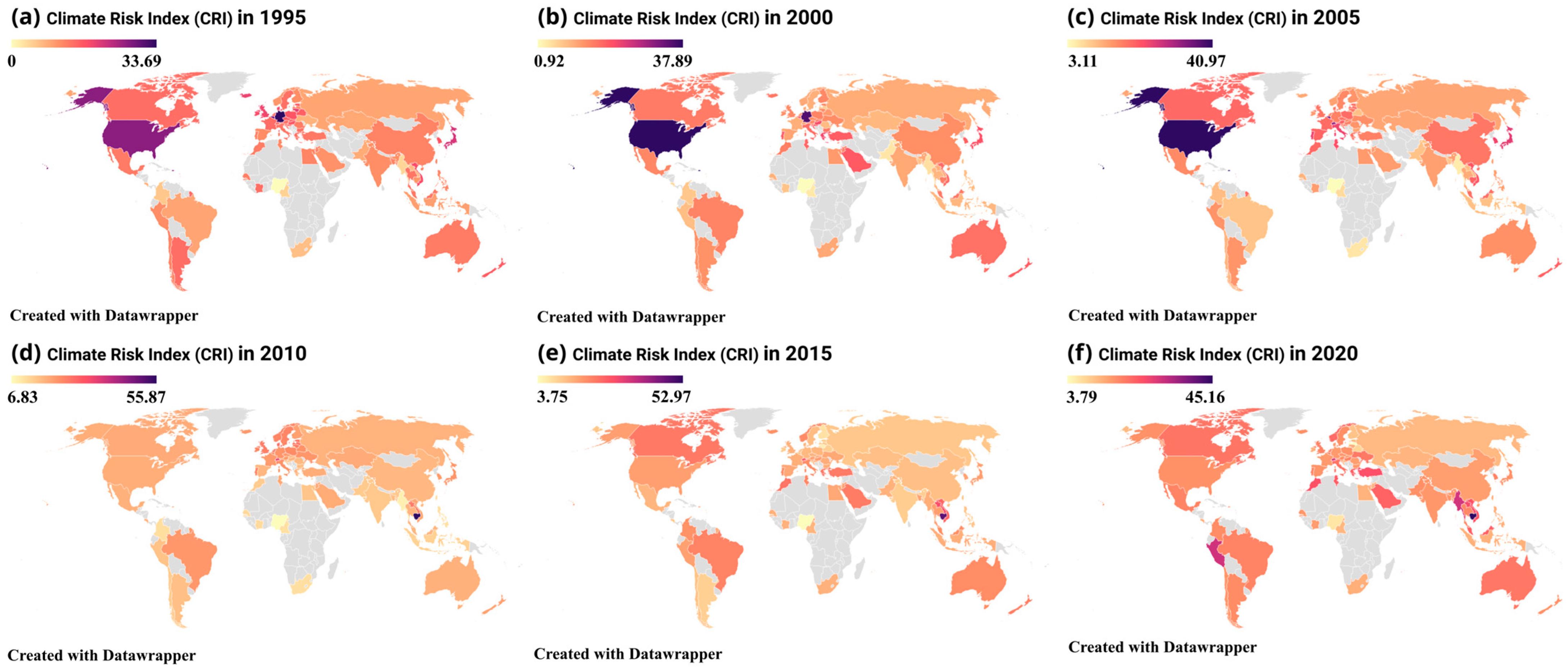
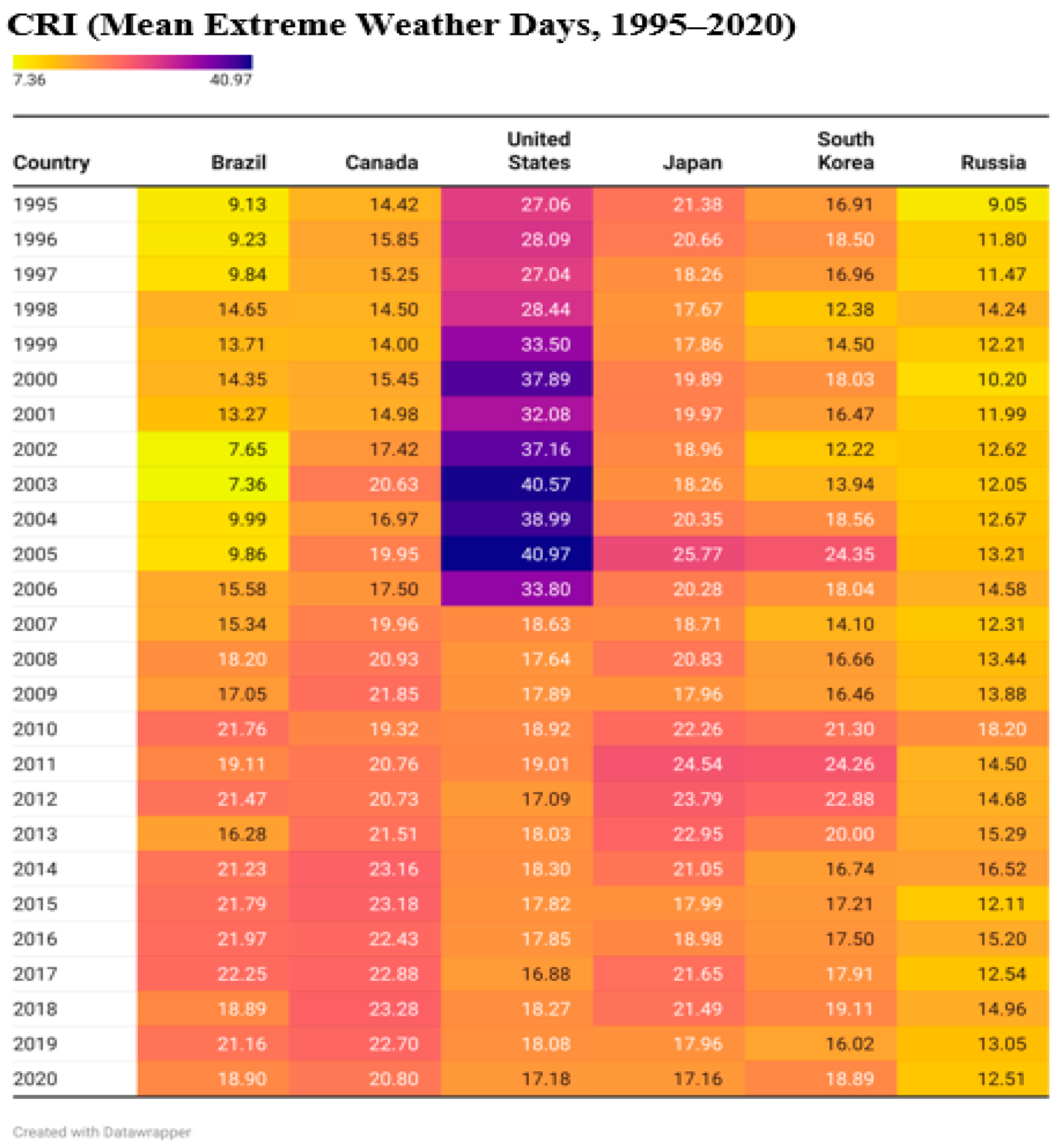
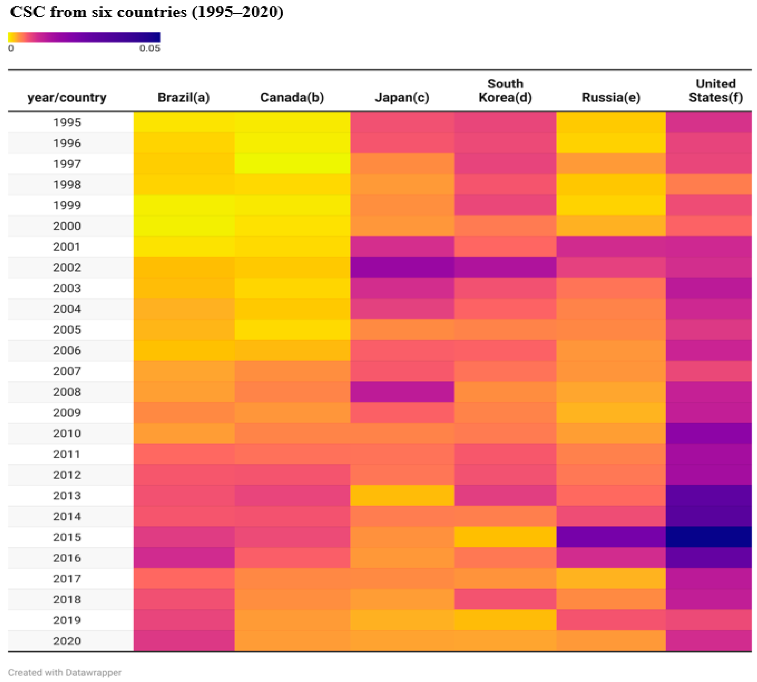
3.1. Intermediate Goods Supply Chain Input-Driven Climate Risk Indicator

The intermediate goods supply chain input-driven climate risk indicator (CSC) for China’s fisheries production sector has shown a steady increase from 1995 to 2020, highlighting a growing exposure to climate risk within the supply chain (Figure 4). After experiencing a decline from 1995 to 1998, with the indicator reaching its lowest value of 0.0447, it began to rise gradually from 1999 to 2002, peaking at 0.1004 in 2002. This upward trend was primarily driven by increased imports from South Korea, Japan, and Russia, all of which faced escalating climate risks. From 2003 to 2015, the indicator continued its ascent, reaching a peak of 0.1577 in 2015, driven by rising demand for intermediate goods in China’s expanding fisheries sector. However, between 2016 and 2017, the indicator saw a sharp decline, largely attributed to a reduction in imports from the United States amid intensifying the United States–China trade tensions. After 2018, the indicator stabilized, reflecting a more balanced supply chain risk environment and reduced volatility from both geopolitical and climate factors.

The CSC for China’s fisheries production sector (1995–2020) is primarily influenced by the United States, Japan, South Korea, Canada, Brazil, and Russia (Figure 5). The indicator from Brazil steadily increased from 1995 to 2016, peaking at 0.0094 in 2016 due to rising climate vulnerabilities affecting key imports (Figure 6a). After 2016, the input-driven climate risk from Brazil declined slightly before stabilizing. The indicator from Canada also increased from 1995 to 2013, peaking at 0.0073 (Figure 6b), then declined and stabilized, following a similar pattern to Brazil but at a lower intensity. In contrast, the indicator from Japan peaked at 0.0163 in 2002 (Figure 6c), then declined steadily and stabilized by 2020, contributing to a reduction in China’s overall input-driven climate risk. The indicator from South Korea followed a similar trend (Figure 6d), peaking at 0.0130 in 2002, with a subsequent decline and stabilization by 2020. The indicator from Russia increased slightly until 2014, peaking at 0.0224 in 2015 (Figure 6e), before declining sharply and stabilizing, reflecting short-term fluctuations. The indicator from the United States exhibited a more volatile trend (Figure 6f), with a sharp rise from 2013 to 2015, peaking at 0.0482 in 2015, which accounted for 30.56% of China’s total input-driven climate risk indicator that year, making it the largest contributor to the overall input-driven climate risk.

Overall, the CSC for China’s fisheries production sector shows an upward trend, with Brazil and Canada contributing to raising the indicator, while Japan and South Korea have seen reduced impacts. Russia and the United States had notable but brief impacts, with the United States playing a pivotal role in the 2015 peak.

3.2. Decomposition of Contribution in the CSC

As shown in Figure 7a, the change in intermediate goods supply chain input-driven climate risk (ΔCSC) from Brazil has steadily increased, particularly after 2001, when the change in the climate risk index (ΔCRI) became the dominant factor. Prior to 2001, changes in dependency (ΔD) and concentration (ΔHHI) had a more significant impact. Figure 7b illustrates that Canada’s ΔCSC also showed an upward trend, with ΔCRI and ΔHHI being the primary drivers. However, since 2013, the influence of dependency (ΔD) has diminished. In the case of Japan (Figure 7c), ΔCSC has been negative, indicating a reduction in climate risk, primarily due to changes in ΔCRI after 2012. South Korea’s ΔCSC (Figure 7d) has had minimal impact, with fluctuations driven mainly by ΔCRI and a decline in dependency since 2015. For the United States (Figure 7e), ΔCSC has been negative since 2015, reflecting a decrease in climate risk. Finally, Russia’s ΔCSC (Figure 7f) has shown little significance, having minimal impact on China’s fisheries production.

In conclusion, the rising climate risk from Brazil and Canada presents challenges to China’s fisheries sector, while Japan and the United States have contributed to mitigating climate risk, benefiting China’s production. The impacts from South Korea and Russia remain minimal, exerting little effect on China’s fisheries. This conclusion aligns with the mechanism verification results presented in Section 3.3.

3.3. Mechanism Verification Results

3.3.1. Mechanism Verification Results for Brazil and Canada

Scenario 1 is supported by the results in

Table 1. Mechanism verification regression results for Brazil and Canada.

	(1)	(2)	(3)		(4)	(5)	(6)
Variables	lny	lnbrdh	lny	Variables	lny	lncadh	lny
lnbrcri	−0.383 * (0.118)	−2.936 (1.299)	−0.173 * (0.0844)	lncandcri	−1.135 * (0.283)	−4.791 * (1.600)	−0.367 (0.149)
lnbrdh			0.0716 *	lncadh			0.160 *
			(0.0132)				(0.0176)
lnchncri	−0.378 *	−5.171	−0.00744	lnchncri	−0.135	−2.748	0.306 *
	(0.203)	(2.234)	(0.146)		(0.201)	(1.139)	(0.100)
lntp	0.0279	0.260	0.00928	lntp	−0.152	−0.304	−0.103
	(0.161)	(1.773)	(0.102)		(0.152)	(0.858)	(0.0662)
lnl	−1.611 *	−21.14	−0.0967	lnl	−0.965	−5.705	−0.0508
	(0.899)	(9.885)	(0.635)		(0.868)	(4.904)	(0.390)
lnk	0.255	5.669	−0.152	lnk	0.236	2.330	−0.138
	(0.409)	(4.490)	(0.269)		(0.362)	(2.044)	(0.162)
lnmj	1.024	8.207 *	0.436	lnmj	0.510	3.150	0.00498
	(0.359)	(3.942)	(0.252)		(0.351)	(1.982)	(0.162)
Constant	10.45	56.52	6.405 *	Constant	7.607	−8.405	8.954 *
	(4.748)	(52.18)	(3.100)		(4.503)	(25.46)	(1.963)
Mediation Effect		54%		Mediation Effect		67.53%
Observations	26	26	26	Observations	26	26	26
R-squared	0.823	0.786	0.933	R-squared	0.851	0.879	0.973

Standard errors in parentheses; *** p < 0.01, ** p < 0.05, * p < 0.1; note: meaning of variables in Appendix A.

, which demonstrate the negative impact of increased climate risk index (CRI) in Brazil and Canada on the output of China’s fisheries sector. In the case of Brazil (columns 1–3), a 1% increase in CRI leads to a 0.383% reduction in China’s fisheries output, a result significant at the 1% level. The decline in the trade of intermediate goods from Brazil, driven by heightened climate risk, significantly affects China’s production, with a net effect of a 0.173% decrease in output, significant at the 10% level. Overall, 54% of Brazil’s climate risk is transmitted through trade. Similarly, for Canada (columns 4–6), a 1% increase in CRI results in a 1.135% decrease in China’s fisheries output, significant at the 1% level. Canada’s climate risk also impacts the production of fisheries-related intermediate goods, contributing a net effect of a 0.367% reduction in output, significant at the 5% level. Notably, 67.53% of Canada’s climate risk is transmitted through trade.

3.3.2. Mechanism Verification Results for Japan and the United States

Scenario 2 is strongly supported by the findings in

Table 2. Mechanism verification regression results for Japan and the United States.

	(1)	(2)	(3)		(4)	(5)	(6)
Variables	lny	lnjapdh	lny	Variables	lny	lnusdh	lny
lnjapcri	1.195 *	5.174 *	0.934	lnuscri	0.321	1.726 *	0.0243
	(0.273)	(1.348)	(0.362)		(0.128)	(0.588)	(0.0979)
lnjapdh			0.0506	lnusdh			0.172 *
			(0.0463)				(0.0317)
lnchncri	−0.986 *	−5.202 *	−0.723	lnchncri	−0.394 *	−0.685	−0.276 *
	(0.216)	(1.063)	(0.322)		(0.220)	(1.007)	(0.141)
lntp	−0.0289	−0.311	−0.0132	lntp	−0.0264	−0.450	0.0509
	(0.142)	(0.698)	(0.142)		(0.174)	(0.798)	(0.111)
lnl	−2.102	1.871	−2.197	lnl	−1.588	−7.139	−0.362
	(0.771)	(3.799)	(0.772)		(0.986)	(4.523)	(0.664)
lnk	0.899 *	−1.014	0.951 *	lnk	0.372	4.497	−0.400
	(0.288)	(1.420)	(0.290)		(0.445)	(2.043)	(0.316)
lnmj	0.997 *	−0.858	1.041 *	lnmj	1.086	6.918 *	−0.101
	(0.316)	(1.556)	(0.316)		(0.389)	(1.785)	(0.330)
Constant	14.54 *	3.080	14.39 *	Constant	11.42	−2.193	11.79 *
	(4.127)	(20.35)	(4.109)		(5.100)	(23.39)	(3.231)
Mediation Effect		22%		Mediation Effect		100%
Observations	26	26	26	Observations	26	26	26
R-squared	0.863	0.615	0.871	R-squared	0.793	0.895	0.921

Standard errors in parentheses; *** p < 0.01, ** p < 0.05, * p < 0.1; note: meaning of variables in Appendix A.

, which indicate that a decline in climate risk index (CRI) in Japan and the United States results in increased output in China’s fisheries sector, primarily through trade in intermediate goods. For Japan (columns 1–3), a 1% decrease in CRI leads to a 1.195% increase in China’s fisheries production, statistically significant at the 1% level. This effect is largely driven by a substantial increase in Japan’s exports of fisheries-related intermediate goods to China. However, only 22% of the positive impact is transmitted through trade, resulting in a net increase of 0.934% in output, which is significant at the 5% level. Despite the limited transmission, Japan’s reduced climate risk has a positive influence on China’s fisheries sector. Similarly, for the United States (columns 4–6), a 1% decrease in CRI boosts China’s fisheries production by 0.312%, significant at the 5% level. This effect is entirely mediated through increased exports of intermediate goods, with 100% of the benefit transmitted via trade, yielding a net increase of 0.172% in output, significant at the 1% level.

3.3.3. Mechanism Verification Results for South Korea and Russia

Scenario 3 is strongly supported by the analysis in

Table 3. Mechanism verification results for South Korea and Russia.

	(1)	(2)	(3)		(4)	(5)	(6)
Variables	lny	lnkrdh	lny	Variables	lny	lnrusdh	lny
lnkrcri	0.516	1.495	0.227	lnruscri	0.0704	0.945	−0.0623
	(0.243)	(0.940)	(0.177)		(0.219)	(1.269)	(0.134)
lnkrdh			0.193 *	lnrusdh			0.140 *
			(0.0405)				(0.0238)
lnchncri	−0.848 *	−3.046	−0.259	lnchncri	−0.476 *	−3.582	0.0263
	(0.293)	(1.133)	(0.235)		(0.262)	(1.513)	(0.179)
lntp	−0.0199	−0.158	0.0106	lntp	−0.0140	−0.308	0.0292
	(0.180)	(0.697)	(0.123)		(0.201)	(1.160)	(0.121)
lnl	−2.656	−7.332 *	−1.239	lnl	−2.184 *	0.442	−2.246 *
	(0.995)	(3.845)	(0.742)		(1.138)	(6.580)	(0.684)
lnk	1.009	3.031	0.423	lnk	1.063	2.112	0.767 *
	(0.365)	(1.409)	(0.278)		(0.404)	(2.335)	(0.248)
lnmj	1.177 *	3.419	0.516	lnmj	0.980	2.730	0.596
	(0.411)	(1.587)	(0.313)		(0.449)	(2.598)	(0.278)
Constant	15.17	19.01	11.50 *	Constant	12.58 *	−33.41	17.27 *
	(5.330)	(20.60)	(3.721)		(6.049)	(34.97)	(3.720)
Mediation Effect		0%		Mediation Effect		0%
Observations	26	26	26	Observations	26	26	26
R-squared	0.777	0.725	0.901	R-squared	0.726	0.641	0.906

Standard errors in parentheses; *** p < 0.01, ** p < 0.05, * p < 0.1; note: meaning of variables in Appendix A.

, which demonstrates that stable climate risk index (CRI) in South Korea and Russia has minimal impact on China’s fisheries production, especially through intermediate goods trade. For South Korea (columns 1–3), slight declines in climate risk lead to a limited positive effect on China’s fisheries output; however, this effect does not propagate through intermediate goods trade. The stability of South Korea’s climate risk from 1995 to 2020, combined with minimal changes in fisheries-related intermediate goods production, explains the weak transmission of effects to China’s fisheries sector. Similarly, for Russia (columns 4–6), the stability of its climate risk results in a negligible impact on China’s fisheries production through intermediate goods trade. While a 1% increase in intermediate goods imports from Russia raises China’s fisheries output by 0.140% (column 6), this effect is not associated with climate risk changes. The stability of Russia’s climate risk underscores the limited influence of climate fluctuations on both intermediate goods trade and production in China’s fisheries sector.

4. Conclusions and Discussion

This study investigates the relationship between climate risk and China’s fisheries production, focusing on how climate fluctuations in key source countries influence the intermediate goods supply chain. By utilizing an intermediate goods trade production function and an input-driven climate risk index, the study offers both theoretical and empirical insights into how climate risks propagate through international trade to impact domestic production. The analysis spans from 1995 to 2020, identifying Brazil, Canada, Japan, the United States, South Korea, and Russia as major contributors to climate-related risks in China’s fisheries sector.

The results show that increased climate risks in Brazil and Canada raise intermediate goods export prices, which negatively affect China’s fisheries output. A 1% increase in climate risk index (CRI) from these countries leads to output reductions of 0.173% and 0.367%, respectively. Conversely, a decline in climate risk from the United States and Japan results in lower intermediate goods costs, benefiting China’s production. A 1% decrease in climate risk index (CRI) from these countries leads to output increases of 0.934% and 0.172%, respectively. For South Korea and Russia, although their climate risk fluctuated, the impact on China’s fisheries production was minimal. However, their exports of intermediate goods positively influenced production, independent of climate fluctuations.

These findings resonate with a growing body of literature emphasizing the transmission of climate risk through global supply chains and its sectoral impacts. The observed negative effect of rising climate risk in Brazil and Canada on China’s fisheries output, mediated by increased intermediate goods prices, aligns with Sun et al. [39], who demonstrated that climate-induced supply shocks in upstream sectors can propagate through trade and production linkages, leading to output volatility across downstream industries, including agriculture and fisheries. Similarly, the magnitude of these effects is quantified by CRI elasticity, which confirms the economic sensitivity of China’s fisheries sector to external environmental risks, echoing Li et al. [40], who found that profitability in China’s aquaculture sector is highly vulnerable to exogenous climate disturbances.

Conversely, the observed benefits associated with declining climate risk in the United States and Japan that manifested through reduced intermediate input costs and improved fisheries output, which are consistent with the risk-mitigation and efficiency-enhancement channels discussed in Chand [41], where reduced climatic uncertainty in key supplier nations contributes to production stability and cost control in China’s marine fisheries. This positive linkage highlights the strategic importance of sourcing diversification and climate resilience in import origins.

The relatively muted impact of climate fluctuations in South Korea and Russia, despite their export contributions, may be interpreted through the lens of Holst and Yu [42], who emphasized that sectoral responses to climate risk vary based on the resilience of domestic production systems and the nature of input dependencies. That their exports contributed positively to production despite climatic variability further supports the assertion by Yao et al. [43] that climate risks do not uniformly translate into output shocks; rather, the effect is contingent upon the volatility spillover intensity and the elasticity of substitution across suppliers.

However, the World Input-Output Table classifies intermediate goods into 45 sectors, which limits the ability to capture specific intermediate goods for fisheries production, such as fishmeal. While China imports fishmeal, about 80% from Peru [44], its relatively low price means that it does not constitute a significant share of China’s total intermediate goods import value in the World Input-Output Table. Therefore, the next step is to disaggregate intermediate goods by specific imported products. This approach would facilitate a more nuanced analysis of how changes in climate risk, transmitted through intermediate goods trade, impact China’s fisheries production.

References

1. Ghadge, A.; Wurtmann, H.; Seuring, S. Managing climate change risks in global supply chains: A review and research agenda. Int. J. Prod. Res. 2019, 58, 44–64. [Google Scholar] [CrossRef]
2. Sussman, F.G.; Freed, J.R. Adapting to Climate Change: A Business Approach; Pew Center on Global Climate Change: Arlington, VA, USA, 2008; Volume 41, Available online: https://www.c2es.org/wp-content/uploads/2008/04/adapting-climate-change-business-approach.pdf (accessed on 1 April 2008).
3. Dasaklis, T.; Pappis, C. Supply chain management in view of climate change: An overview of possible impacts and the road ahead. J. Ind. Eng. Manag. 2013, 6, 1139–1161. [Google Scholar] [CrossRef]
4. Dawson, J.; Holloway, J.; Debortoli, N.; Gilmore, E. Treatment of International Economic Trade in Intergovernmental Panel on Climate Change (IPCC) Reports. Curr. Clim. Change Rep. 2020, 6, 155–165. [Google Scholar] [CrossRef]
5. Kara, M.; Ghadge, A.; Bititci, U. Modelling the impact of climate change risk on supply chain performance. Int. J. Prod. Res. 2020, 59, 7317–7335. [Google Scholar] [CrossRef]
6. Brander, K. Global fish production and climate change. Proc. Natl. Acad. Sci. USA 2007, 104, 19709–19714. [Google Scholar] [CrossRef]
7. Free, C.M.; Thorson, J.T.; Pinsky, M.L.; Oken, K.L.; Wiedenmann, J.; Jensen, O.P. Impacts of historical warming on marine fisheries production. Science 2019, 363, 979–983. [Google Scholar] [CrossRef] [PubMed]
8. Chang, Y.; Lee, M.; Lee, K.; Shao, K. Adaptation of fisheries and mariculture management to extreme oceanic environmental changes and climate variability in Taiwan. Mar. Policy 2013, 38, 476–482. [Google Scholar] [CrossRef]
9. Caputi, N.; Kangas, M.; Denham, A.; Feng, M.; Pearce, A.; Hetzel, Y.; Chandrapavan, A. Management adaptation of invertebrate fisheries to an extreme marine heat wave event at a global warming hot spot. Ecol. Evol. 2016, 6, 3583–3593. [Google Scholar] [CrossRef]
10. Do, V.; Phung, M.; Truong, D.; Pham, T.; Dang, V.; Nguyen, T. The impact of extreme events and climate change on agricultural and fishery enterprises in Central Vietnam. Sustainability 2021, 13, 7121. [Google Scholar] [CrossRef]
11. PwC. International Threats and Opportunities of Climate Change to the UK: Report Prepared for the UK Department for Environment, Food and Rural Affairs (Defra); Price Water House Coopers LLP: London, UK, 2013; pp. 149–203. [Google Scholar]
12. Merino, G.; Barangé, M.; Mullon, C. Climate variability and change scenarios for a marine commodity: Modelling small pelagic fish, fisheries and fishmeal in a globalized market. J. Mar. Syst. 2010, 81, 196–205. [Google Scholar] [CrossRef]
13. Yasmin, R.; Islam, M. Sustainability of fisheries and aquaculture in context of emerging climate change issues. Int. J. Fish. Aquat. Stud. 2017, 5, 176–187. [Google Scholar]
14. Hall, G. Impact of climate change on aquaculture: The need for alternative feed components. Turk. J. Fish. Aquat. Sci. 2015, 15, 569–574. [Google Scholar] [CrossRef] [PubMed]
15. Teng, P.; Lassa, J.; Caballero-Anthony, M. Climate change and fish availability. COSMOS 2016, 12, 29–42. [Google Scholar] [CrossRef]
16. Fleming, A.; Hobday, A.; Farmery, A.; van Putten, E.; Pecl, G.; Green, B.; Lim-Camacho, L. Climate change risks and adaptation options across Australian seafood supply chains—A preliminary assessment. Clim. Risk Manag. 2014, 1, 39–50. [Google Scholar] [CrossRef]
17. Allison, E.; Perry, A.; Badjeck, M.; Adger, W.; Brown, K.; Conway, D.; Halls, A.; Pilling, G.; Reynolds, J.; Andrew, N.; et al. Vulnerability of national economies to the impacts of climate change on fisheries. Fish Fish. 2009, 10, 173–196. [Google Scholar] [CrossRef]
18. Sumaila, U.; Cheung, W.; Lam, V.; Pauly, D.; Herrick, S. Climate change impacts on the biophysics and economics of world fisheries. Nat. Clim. Change 2011, 1, 449–456. [Google Scholar] [CrossRef]
19. Marshak, A.; Link, J. Primary production ultimately limits fisheries economic performance. Sci. Rep. 2021, 11, 12154. [Google Scholar] [CrossRef]
20. Gurgel, C.; Camacho, O.; Minne, A.; Wernberg, T.; Coleman, M. Marine heatwave drives cryptic loss of genetic diversity in underwater forests. Curr. Biol. 2020, 30, 1199–1206.e2. [Google Scholar] [CrossRef]
21. Pujolar, J.; Vincenzi, S.; Zane, L.; Jeseňsek, D.; Leo, G.; Crivelli, A. The effect of recurrent floods on genetic composition of marble trout populations. PLoS ONE 2011, 6, e23822. [Google Scholar] [CrossRef]
22. Gray, S.; Dermody, O.; Klein, S.; Locke, A.; McGrath, J.; Paul, R.; Rosenthal, D.; Ruiz-Vera, U.; Siebers, M.; Strellner, R.; et al. Intensifying drought eliminates the expected benefits of elevated carbon dioxide for soybean. Nat. Plants 2016, 2, 16132. [Google Scholar] [CrossRef]
23. Stokeld, E.; Croft, S.; dos Reis, T.N.; Stringer, L.C.; West, C. Stakeholder perspectives on cross-border climate risks in the Brazil-Europe soy supply chain. J. Clean. Prod. 2023, 428, 139292. [Google Scholar] [CrossRef]
24. Rezaee, S.; Pelot, R.; Ghasemi, A. The effect of extreme weather conditions on commercial fishing activities and vessel incidents in Atlantic Canada. Ocean Coast. Manag. 2016, 130, 115–127. [Google Scholar] [CrossRef]
25. Bednar, F.B.; Knittel, N.; Raich, J.; Adams, K.M. Adaptation to transboundary climate risks in trade: Investigating actors and strategies for an emerging challenge. WIREs Clim. Change 2022, 13, e758. [Google Scholar] [CrossRef]
26. Carter, T.; Benzie, M.; Campiglio, E.; Carlsen, H.; Fronzek, S.; Hildén, M.; Reyer, C.P.; West, C. A conceptual framework for cross-border impacts of climate change. Glob. Environ. Change 2021, 69, 102307. [Google Scholar] [CrossRef]
27. Tang, Y.; Zou, W.H.; Hu, Z.M. An analysis of utilization status and management of marine fisheries resources in china based on statistics data. Resour. Sci. 2009, 31, 1061–1068. (In Chinese) [Google Scholar]
28. Yang, Z.J. Evaluation of the contribution of technological progress in China’s fishery industry based on TFP measurement. In Proceedings of the 2011 China Fisheries Economics Expert Forum, Beijing, China, 21–22 June 2011; Chinese Academy of Fishery Sciences: Beijing, China, 2011; p. 10. (In Chinese). [Google Scholar]
29. Zhang, T. Research on the Changes in Total Factor Productivity and Regional Convergence of China’s Fishery Industry. Doctoral Dissertation, Zhejiang Ocean University, Zhoushan, China, 2021; pp. 1–43. (In Chinese). [Google Scholar]
30. Guo, K.; Ji, Q.; Zhang, D. A dataset to measure global climate physical risk. Data Brief 2024, 54, 110502. [Google Scholar] [CrossRef] [PubMed]
31. Jones, M.; Dye, S.; Pinnegar, J.; Warren, R.; Cheung, W. Using scenarios to project the changing profitability of fisheries under climate change. Fish Fish. 2015, 16, 603–622. [Google Scholar] [CrossRef]
32. Suh, D.; Pomeroy, R. Projected economic impact of climate change on marine capture fisheries in the Philippines. Front. Mar. Sci. 2020, 7, 232. [Google Scholar] [CrossRef]
33. Nguyen, T. Welfare impact of climate change on capture fisheries in Vietnam. PLoS ONE 2022, 17, e0264997. [Google Scholar] [CrossRef]
34. Cripps, M.W.; Myles, G.D. General equilibrium and imperfect competition: Profit feedback and price normalization. Res. Agric. Appl. Econ. Work. Pap. 1988, 295. [Google Scholar] [CrossRef]
35. Wagner, S.M.; Bode, C. An empirical investigation into supply chain vulnerability. J. Purch. Supply Manag. 2006, 12, 301–312. [Google Scholar] [CrossRef]
36. Su, Q. Analysis of the relationship between security and efficiency in global supply chains. Int. Political Sci. 2021, 6, 1–32. (In Chinese) [Google Scholar]
37. Zhu, J.L.; Fang, Y. Multilateral Trade Cooperation and the “Stabilization Chain” of Chinese Manufacturing under the Dynamic Global Trade Pattern—Based on the Estimation of Production Risk Sources in China’s Manufacturing Supply Chain. Quant. Econ. Tech. Econ. Res. 2024, 41, 89–111. (In Chinese) [Google Scholar]
38. Rubinstein, A. Modeling Bounded Rationality; Zeuthen Lecture Book Series; MIT Press: Cambridge, MA, USA, 1988; Volume 220, pp. 1–208. [Google Scholar] [CrossRef]
39. Sun, Y.; Zou, X.; Shi, X.; Zhang, P. The economic impact of climate risks in China: Evidence from 47-sector panel data, 2000–2014. Nat. Hazards 2024, 95, 289–308. [Google Scholar] [CrossRef]
40. Li, S.; Yang, Z.; Nadolnyak, D.; Zhang, Y.; Luo, Y. Economic impacts of climate change: Profitability of freshwater aquaculture in China. Aquac. Res. 2016, 47, 1537–1548. [Google Scholar] [CrossRef]
41. Chand, A. China’s marine fisheries and climate risks. Nat. Food 2024, 5, 4. [Google Scholar] [CrossRef]
42. Holst, R.; Yu, X. Climate Change and Production Risk in Chinese Aquaculture. Courant Research Centre Discussion Papers 2011, No. 64. Available online: https://hdl.handle.net/10419/90469 (accessed on 20 April 2025).
43. Yao, Z.; Chen, Y.; Deng, S.; Zhang, Y.; Wei, Y. Carbon emission allowance, global climate risk, and agricultural futures: An extreme spillover analysis in China. Financ. Res. Lett. 2025, 71, 106391. [Google Scholar] [CrossRef]
44. Calderón, R.G.; Brunella, B.; Llatas, H.; Delicia, F. Perú fishmeal exports, 2018–2022. In Proceedings of the Latin American and Caribbean Conference for Engineering and Technology, San José, Costa Rica, 17–19 July 2024; pp. 1–11. [Google Scholar] [CrossRef]
Figure 1. Trends in climate risk index (CRI) for countries. (Gray and white areas represent missing values. The darker the color, the higher the climate risk).
Fishes 10 00210 g001
Figure 2. Trends in climate risk index (CRI) of six countries for imported intermediate goods of China’s fisheries sector. (The darker the color, the higher the CRI).
Fishes 10 00210 g002
Figure 3. Mechanism verification logic diagram. (a is the coefficient of CRI in Formula (26); b is the coefficient of DH in Formula (27); c is the coefficient of CRI in Formula (25); c′ is the coefficient of CRI in Formula (27)).
Fishes 10 00210 g003
Figure 4. Trend of CSC in China’s fisheries production sector. (The larger the line length, the greater the CSC).
Fishes 10 00210 g004
Figure 5. The CSC from 78 countries (regions) for China’s fisheries production sector, 1995–2020. (The larger the bubble, the greater the CSC originating from each country (region)).
Fishes 10 00210 g005
Figure 6. Trends of the CSC from six countries. (The darker the color, the higher the CSC).
Fishes 10 00210 g006
Figure 7. Contribution decomposition of changes in the CSC from six countries. (Figure 7a, 7b, 7c, 7d, 7e and 7f are the contribution decomposition of changes in the CSC from Brazil, Canada, Japan, Korea, United States and Russia, respectively).
Fishes 10 00210 g007