Article

Enhancing Management Strategy Evaluation: Implementation of a TOPSIS-Based Multi-Criteria Decision-Making Framework for Harvest Control Rules

Department of Geography, Texas A&M University, College Station, TX 77843, USA
*
Author to whom correspondence should be addressed.
Fishes 2025, 10(4), 140; https://doi.org/10.3390/fishes10040140
Submission received: 7 February 2025 / Revised: 12 March 2025 / Accepted: 17 March 2025 / Published: 21 March 2025
(This article belongs to the Section Fishery Economics, Policy, and Management)

Abstract

Management Strategy Evaluation (MSE) tools are inspired by the need for transparency, efficiency, and collaboration in harvest control rule (HCR) management. MSEs provide quantified metrics of the HCR performances and indicate the goodness in multiple dimensions, but providing HCR rankings based on such criteria is uncommon or use a simple Weight Sum Method (WSM). Acknowledging some theoretical limitations of the WSM, we propose using Technique for Order Preference by Similarity to Ideal Solution Method (TOPSIS) as an efficient alternative algorithm for recommending HCRs and conduct a sensitivity analysis of management objectives under the two frameworks, one based on simulated history and the other on the history of North Pacific Albacore (NPALB). Two conclusions are drawn based on the computation of the HCR ranking differences generated with the WSM and TOPSIS: (1) The alteration in the overall ranking of HCRs is visible, and its influence could vary substantially with user preference with theoretical merits. (2) It is common to notice shifts in the ranking for top HCRs, which potentially contributes valuable insights for practical decision making.
Key Contribution: TOPSIS provides significantly different HCR recommendations from the ones by WSM, and it could suggest decision support merits for fishery management in strategy adaptation.

1. Introduction

Harvest control rules (HCRs) are established sets of fishing guidelines that regulate macro-level activity intensity for all parties involved through monitoring relevant biomass metrics. These collaborative rules represent a common ground where parties of occasionally conflicting interests share the numerical boundaries for different sets of commercial fishing practices. HCRs operationalize high-level, conceptual directives through the quantification of objectives and the compilation of estimation models, formulae, and inputs of field knowledge. The installation of HCRs guarantees the consistency, transparency, and scientific foundation of fishery decision making on an actionable level. Although the implementation of these HCRs varies in forms in different regions in the US, a common goal would be the Maximum Sustainable Yield in a given biomass. In particular, threshold-based HCRs often employ target reference points (TRPs) and limit reference points (LRPs), representing the ideal, healthy state and the unsustainable, overfished state of the target fish stock, respectively [1]. Threshold-based HCRs are widely employed in different US fishing communities and for different species, and a recent study suggested that for some species, threshold HCRs outperform other complex forms of HCRs [2,3]. Many of these HCRs are represented in the “Hockey Stick” graphs, an example of which is presented in Figure 1.

1.1. Management Strategy Evaluation Tools

Management Strategy Evaluation (MSE) aims to provide an evaluative analysis of a user-defined HCR through the integration of projected annual catch and annual fish population into the future while simulating their interactions. More specifically, an MSE utilizes the following elements to achieve its purposes:
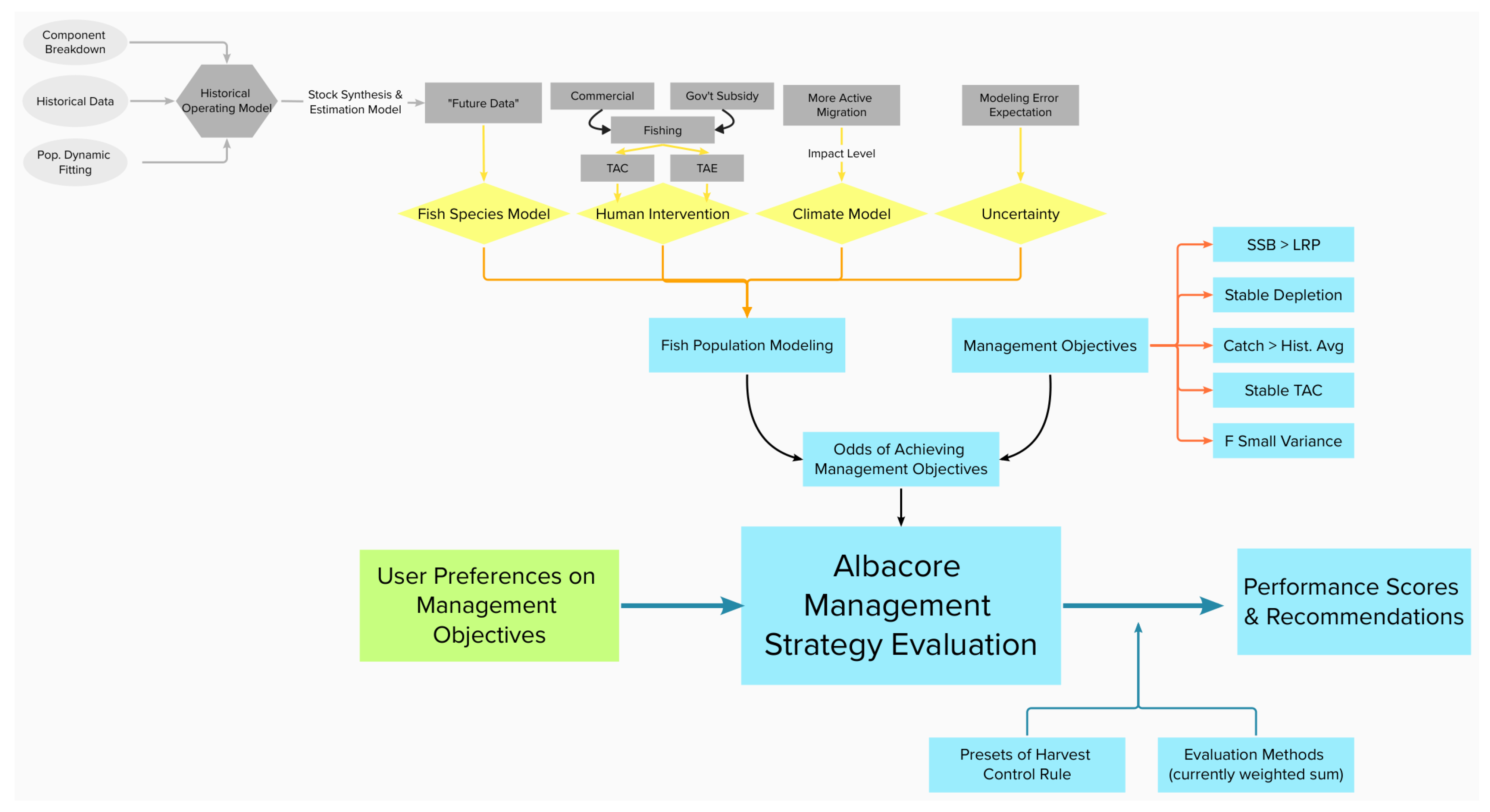
  • An Operation Model. An operation model reads in historical data for the “ground truth” fish biomass and simulates the population dynamics through fish population models.
  • An Estimation Model. An estimation model is based on the operation model and projects the future fish biomass and fish catch, iteratively generating estimated values based on defined parameters.
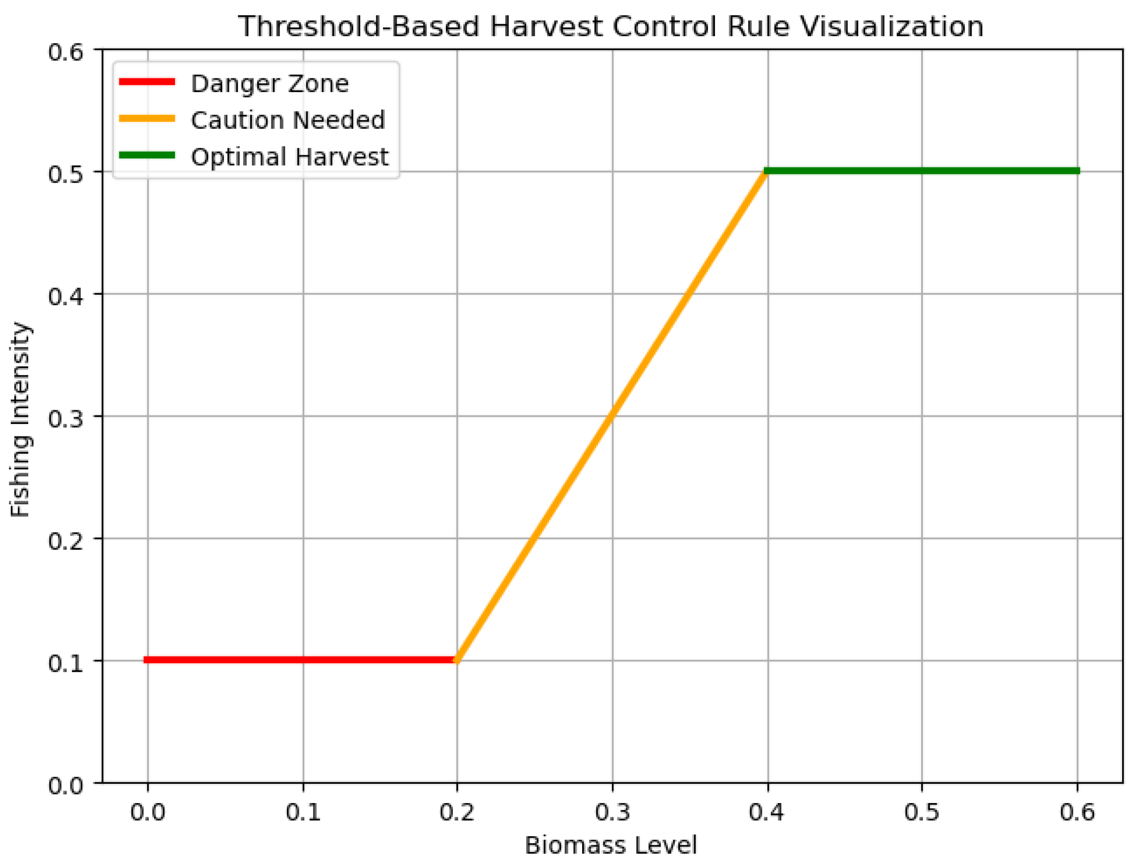
  • An HCR. The MSE takes in the parameters, e.g., TRP, LRP, and maximum catch, and simulates the regulatory effect of an HCR in the catch, thus further impacting the fish biomass projection.
With these elements, the MSE is able to generate “future data” and thus evaluate the HCR in multiple dimensions, which is essentially how well it achieves user-defined management objectives in any applicable target time period, with some examples including fish catch, biomass, fishing effort, etc. [1]. The evaluative properties may vary depending on implementation, but they are always quantitative and open for further aggregation. With this said, many current implementations of MSEs often stop at this stage and leave the HCR recommendation system open for further context. One implementation we would like to examine closely is the North Pacific Albacore MSE by the International Scientific Committee for Tuna and Tuna-Like Species in the North Pacific Ocean (ISC); the decision support system gives a Weighted Sum Method (WSM) to provide a trade-off demonstration for different aspects of HCR (e.g., a higher priority for catch could result in biomass loss) [4]. An introduction for this tool is provided in Section 1.2.

1.2. Implementation of North Pacific Albacore MSE by the ISC

In this section, a brief introduction of the North Pacific Albacore (NPALB) species and the interactive decision support web tool for NPALB by the ISC will be provided because it gives a concrete case of how MSE tools are adapted for a fish species and produce evaluative metrics.
The North Pacific Albacore tuna (Thunnus alalunga) is considered a reproductively isolated fish stock with respect to the South Pacific stock, supported by various sets of data, including tagging, genetic data, and many more [6,7]. It is considered a slow-growing species with an extended lifespan among all fish and thus could be more heavily influenced by excessive fishing practices [8,9,10,11]. The age and growth are modeled with a von Bertalanffy growth function that features quick growth during a small age and an ensuing flattened curve with parameters ( L , K , t 0 ) = (124.1 cm, 0.164 year 1 , −2.239 years) [12]. Recently, climate change in the Pacific Ocean has influenced its harvesting strategy. Three representative fish species on the West Coast, sardines (Sardinops sagax caerulea), swordfish (Xiphias gladius), and albacore tuna, are expected to migrate toward the North Pole due to climate change; compared to the other two, albacore tuna are migratory species, projected to migrate longer distances, and thus are increasingly being relied upon by the Southern fishing community to make up for the loss [13].
Albacore tuna has a long history of being a valuable commercial fish stock in the North Pacific Fishery [14]. More recently, from 2011 to 2015, Japan was the leading fishing community, responsible for 61.9% of all North Pacific albacore tuna harvest, with the United States for 16.9%, Canada for 5.4%, and China for 4.3%. Table 1 provides records of North Pacific Albacore tuna fish catch in pounds and its values in dollars from the U.S., 2010 to 2022 [15].
The MSE takes in pre-collected relevant biomass data, aggregates models, and evaluates North Pacific Albacore harvesting strategies given a collection of management objectives agreed upon by stakeholders and industry managers [14]. This tool covers specifically North Pacific Albacore species and was developed in order to both provide a traceable fish population predictive model and further examine an optimal TRP and an HCR. The HCRs are divided into two major guiding quotas: total allowable catch (TAC) and total allowable effort (TAE). In this formulation, the TAE is not employed and evaluated individually; HCRs with the TAE are accessed in a mixed control case [14]. The MSE uses a population dynamic model of albacore tuna embedded in a back-end simulation system that includes a management module to simulate the biomass of albacore tuna and its fisheries 30 years in the future under 128 different harvest control rules [16]. Based on relevant parameters produced by the operation model and the estimation model, each HCR generates management objective metrics, including Spawning Stock Biomass (SSB), annual catch, etc. [14]. Specifically, there are five such management objectives, collaborated and agreed upon by the Inter-American Tropical Tuna Commission (IATTC) and the Western and Central Pacific Fisheries Commission (WCPFC). All of them are evaluated quantitatively with probabilities or normalized data:
  • Maintain an SSB higher than the limit reference point (LRP);
  • Maintain the depletion of total biomass around the historical average depletion;
  • Maintain catches above the average historical catch;
  • The change in the total allowable catch between years should be relatively gradual;
  • Maintain fishing intensity (F) at the target reference point with reasonable variability.
Figure 2 demonstrates how the MSE and fish population dynamic toolkits work together [4]. The tool first produces a back-end simulation that models the fish population, taking various components into account, including but not limited to fish species dynamics, human intervention, climate modeling, and estimation errors. The MSE then provides necessary metrics and allows for a quantitative analysis of the probability of achieving management objectives. These probabilities are collectively transformed into odds and considered parameters for HCRs. With these preset HCRs and their respective odds, the MSE web tool collects user-assigned weights, performs its evaluation method (currently the WSM), yields final performance scores of all HCRs, and recommends the HCR with the highest final score.

1.3. Limitations of the Weighted Sum Method and Motivation for a New Decision Support Model

In this section, the limitations of the simple WSM in the context of providing decision support on recommending fishery HCRs will be briefly discussed based on its mathematical properties. Section 2.2 provides a formal mathematical introduction for the WSM. However, in short, the WSM computes a score for each alternative through summing the products of the user’s weights for each criterion and the respective criterion value. The advantages of the WSM are its intuitive structure, simple implementation, and very low computational cost.
There are three limitations, however, when the WSM is put into the HCR recommendation context. First, the linear additive form of the sum implies a highly unclear yet influential compensation scheme, i.e., the evaluation of the HCR could make up for its very poor performance in one particular objective with good performances in other objectives. Such invisible deception could easily be problematic in a decision-making context since, usually, the decision makers not only want to maximize gains but also to avoid extremely bad circumstances, e.g., there is a very high risk of breaking the LRP compensated for by a very high Catch Per Unit Effort (CPUE). When only the WSM scores are inspected, it becomes unclear whether this extreme case has happened or not. Second, the WSM projects each objective metric into the linear space and loses the structure as well as the awareness of other alternatives in the early stage of the aggregation. This dimensional collapse limits the reflection of the referential and comparative properties against other possible alternatives. Third, it is essentially hard to put the final WSM scores into context since they do not directly translate into quantitative scales or relative proportions to relatable standards; it is simply a metric of goodness.
Inspired by the gaps in the HCR recommending system, this study proposes using the Technique for Order Preference by Similarity to Ideal Solution (TOPSIS) method as an alternative to the WSM [17,18]. The purpose of this study is to illustrate both the theoretical differences and the distinctions between the outputs generated by applying the WSM in MSE systems and the ones from TOPSIS. It should be noted that this study does not wish to assert TOPSIS’s supremacy but merely display the dissimilarity.
In addition, the contribution of each objective to the final ranking of HCRs currently remains unclear, and finding out how some objectives may influence the outcome more significantly could also be covered. For this reason, a sensitivity analysis that investigates the relationship between each management objective performance scoring and the changes in HCR rankings was conducted to further understand the decision-making process.

2. Materials and Methods

2.1. Theoretical Background

2.1.1. Multi-Criteria Decision Making (MCDM)

Multi-criteria decision making is an analytical framework that utilizes a variety of mathematical models that provide decision support when multiple goals need to be considered and optimized at the same time, extensively realized in various fields of study [19]. It serves as an important part of the analytical framework under various disciplines, such as disaster response and recovery and multi-objective routing [20,21].
Usually, given a set of alternative candidates, an MCDM method would perform an evaluation of each alternative based on its performance on the objectives and users’ preferences. A final ranking of these alternatives will be provided based on the evaluation. In this study, the WSM and TOPSIS are implemented and compared.

2.1.2. Weighted Sum Method (WSM)

Consider m alternatives and n objectives. Then, the performance metric P i of the i-th alternative is evaluated based on the following expression:
P i = j = 1 n x i j w j
where x i j is the performance of the j-th alternative on the i-th objective, and w i is the weight assigned to the i-th objective. Usually, the WSM will normalize the objective performance parameters to make user weights more reflective. After the evaluation, the best alternative is selected by the ranking of the performance metric P i , the higher the better.

2.1.3. Technique for Order Preference by Similarity to Ideal Solution (TOPSIS) Method

TOPSIS was proposed in 1981, further refined in the following years by the authors and other contributors, and has been actively popularized in various multi-criteria decision support contexts [17,22,23,24]. On a high level, the TOPSIS method develops sets of positive ideal and negative ideal alternatives based on the objective scores. Then, it iterates through the set of actual alternatives and locates the one that is closest to the positive ideal and farthest from the negative ideal. This method provides unique insights when the positive and negative ideal scenarios of the proposed objectives are exceedingly more important than the linearly aggregated benefits, and for this reason, it has affinity to policy decision making in HCR settings—the policymakers are more interested in achieving the closest distances to ideal states of objective metrics (e.g., catch, stability) and simultaneously the farthest distances to the negative ideal states of objectives (e.g., minimizing distance to the TRP to avoid the risk of breaching the LRP).
Formally, for m alternatives and n objectives, the TOPSIS method comprises the following steps [18]:
  • Construct a normalized decision matrix r such that each entry in the matrix is calculated as follows:
    r i j = x i j x i j 2   for   i = 1 , , m   and   j = 1 , , n
    where x i j is the respective performance score of the i-th alternative on the j-th parameter.
  • Construct a weighted normalized decision matrix v i j with the following expression:
    v i j = w j r i j
    where w j is the weight assigned to the j-th objective.
  • Determine the positive and the negative ideal alternative from the previous matrix as follows:
    Positive:
    A P = { v 1 P , , v n P }
    where v j P = { m a x ( v i j ) i f j J ; m i n ( v i j ) i f j J }
    Negative:
    A N = { v 1 N , , v n N }
    where v j N = { m i n ( v i j ) i f j J ; m a x ( v i j ) i f j J }
  • For each alternative, calculate its separation from the ideals with the following:
    Separation from positive ideal:
    S i P = [ i = 1 m ( v j P v i j ) 2 ] 1 2
    Separation from negative ideal:
    S i N = [ i = 1 m ( v j N v i j ) 2 ] 1 2
  • For each alternative, calculate its final relative closeness to ideals C i with the following:
    C i = S i N S i P + S i N
    The alternative with highest relative closeness is considered the best by the algorithm, given the user’s preferences, the objectives, and the alternatives’ performances.
The TOPSIS method has the following characteristics in multi-criteria decision making due to its formulation:
  • Preservation of multi-dimensional analytical structure until the last step. The TOPSIS method evaluates each alternative through comparisons between each of its objective parameters and the polarized ideal states. This characteristic ensures consistent geometric awareness of the underlying disparate data distributions across different objectives during evaluation.
  • Geometric assessment. While TOPSIS remains a compensatory framework, i.e., allowing alternatives to make up disadvantages with strengths, its formulation with distance implies that deviation from the ideals is squared and thus more penalized compared to linear models such as the WSM. In other words, those alternatives with extremely poor performance in any objective will be more visibly demonstrated in their TOPSIS scores; the worse the performance, the heavier the penalty. This characteristic significantly reduces the chances of TOPSIS to rank imbalanced alternatives as better ones. On the other hand, since the distance is spread out on a ( 0 , 1 ) range through geometric calculation, it would also tend to nuance the alternatives when aggregated and lower the chance of producing ties.
  • Results in the scales of ideal alternatives. Due to its construction of the comparisons with respect to the best possible scenarios, the evaluative metrics could be explained in relative relationships, e.g., closeness to the ideal circumstances. This could potentially improve the explainability of the output due to its contextual relevance, while results from other formulations, such as aggregated WSM scores, cannot easily translate to sensible knowledge.

2.1.4. Sensitivity Analysis

Sensitivity analysis is an important step in MCDM that digs deeper into the significance of each objective in the final ranking of the alternatives. Through understanding their contribution to the ranking, there could be more insights into the contextual priorities. Specifically, the sensitivity analysis evaluates to what extent a set of parameters influences the output of the target parameters. In this study, a range of applicable weights was employed to understand the prominence of each objective when the decision priority was produced through Sobol’s Methods. A high-level example of surveying the sensitivity of NPALB objectives is to define the ranges of weights for each, e.g., from 1 to 5, allocate these ranges to their respective objectives, define the target variable (which would be the change in the HCR rankings in this case), and sample the defined number of simulations, e.g., 1024 runs. From these results, the distribution is inspected and compared to locate the power of each component.
Sobol’s Method, or variance-based sensitivity analysis, provides a global sensitivity evaluation through calculating the ratio between output and input variances, is facilitated via Monte Carlo simulation, and provides computational strength in non-linear scenarios [25,26].

2.2. Data Collection and Processing

This study collected results from two online MSE tools that provide performance metrics for given HCRs. After the aggregation of metrics, the WSM and TOPSIS were run independently on the dataset to generate respective recommendations. Then, the results were compared based on the rankings of the HCRs.

2.2.1. AMPLE MSE

Amazing Management Procedures expLoration Engine (AMPLE) was created and maintained by The Pacific Community (SPC) and provides three Shiny apps relevant to the evaluation of HCRs: one for introducing HCRs, one for measuring HCRs, and one for comparing HCRs [5]. The implementation is in the R language with an open source GitHub repository [27]. The tool is not based on any fish species data; it generates a random starting point and the ensuing historical biomass and fish catch as its hypothetical operational model database. For the Measuring HCR Performance interface, the tool requires inputs from the user to define an HCR through four parameters: Blim, Belbow, Cmin, and Cmax (corresponding to the LRP, TRP, minimum catch, and maximum catch, respectively). Then, the MSE generates an estimation of the fish stock and catch level into three future stages: short, medium, and long. For each period, the study aggregates relevant data and produces its performance metrics in six dimensions: (1) the probability that biomass is greater than the LRP, (2) estimated catch, (3) relative Catch Per Unit Effort, (4) relative effort, (5) catch stability, and (6) proximity to the TRP. The user may also choose to include variability parameters in the simulation to account for uncertainty and bias in the biological and predictive processes. Three types of variability parameters are available from 0 to 1: (1) biological variability, (2) estimation variability, and (3) estimation bias.
Test data were collected from the website with the following settings:
  • The HCR inputs have the following options to choose from:
    (a)
    Blim: One value from (0.2, 0.25, 0.3, 0.4).
    (b)
    Belbow: One value from (0.6, 0.8).
    (c)
    Cmin: One value from (50, 75).
    (d)
    Cmax: One value from (125, 200).
    In total, this constitutes a compilation of 32 HCRs as competing alternatives. The complete permutation table of their performances is provided in Appendix A.
  • The variability inputs: All variability inputs were set to 0.1.
  • The HCR type was set to the threshold catch.
  • The simulation was run at least 30 times, and a representative run from these runs was manually selected to collect performance metrics.
  • The medium time period was the only considered set of performance metrics. The exclusion of datasets from short and long periods was due to the need for comparative simplicity.
  • Stock life history was set to medium growth; stock history was set to be fully exploited; other settings were set to default values.
  • Software was accessed in February 2025, Version 1.0.0.
In the end, a CSV file with the specifications of the HCRs and their respective performance metrics was prepared for the WSM and TOPSIS runs.

2.2.2. NPALB MSE

This study collected the performance metrics of the targeted HCRs from the technical reports from the ISC in 2021, which is an aggregated result from the Operation and Estimation Model conditioned on historical North Pacific Albacore tuna data from 1993 to 2015 [14]. Since 2000, the US enacted the Dolphin-Safe Tuna Tracking and Verification Program to create records of nationwide frozen and processed tuna products managed under multiple fishery plans to ensure appropriate participants and fishing intensity [11]. Due to its migratory nature, this species is internationally managed by the Inter-American Tropical Tuna Commission (IATTC) and the Western and Central Pacific Fisheries Commission (WCPFC), while significant participating fleets include the Japanese, US, Chinese Taipei, and Canadian fleets [11,28]. Performance metrics were individually evaluated and organized into two separate Excel files according to their harvest type, being TAC or mixed control. Specifically, this study took a closer look at the 16 TAC threshold-based HCRs and their performance metrics. The specifications of these HCRs are provided in Appendix C.

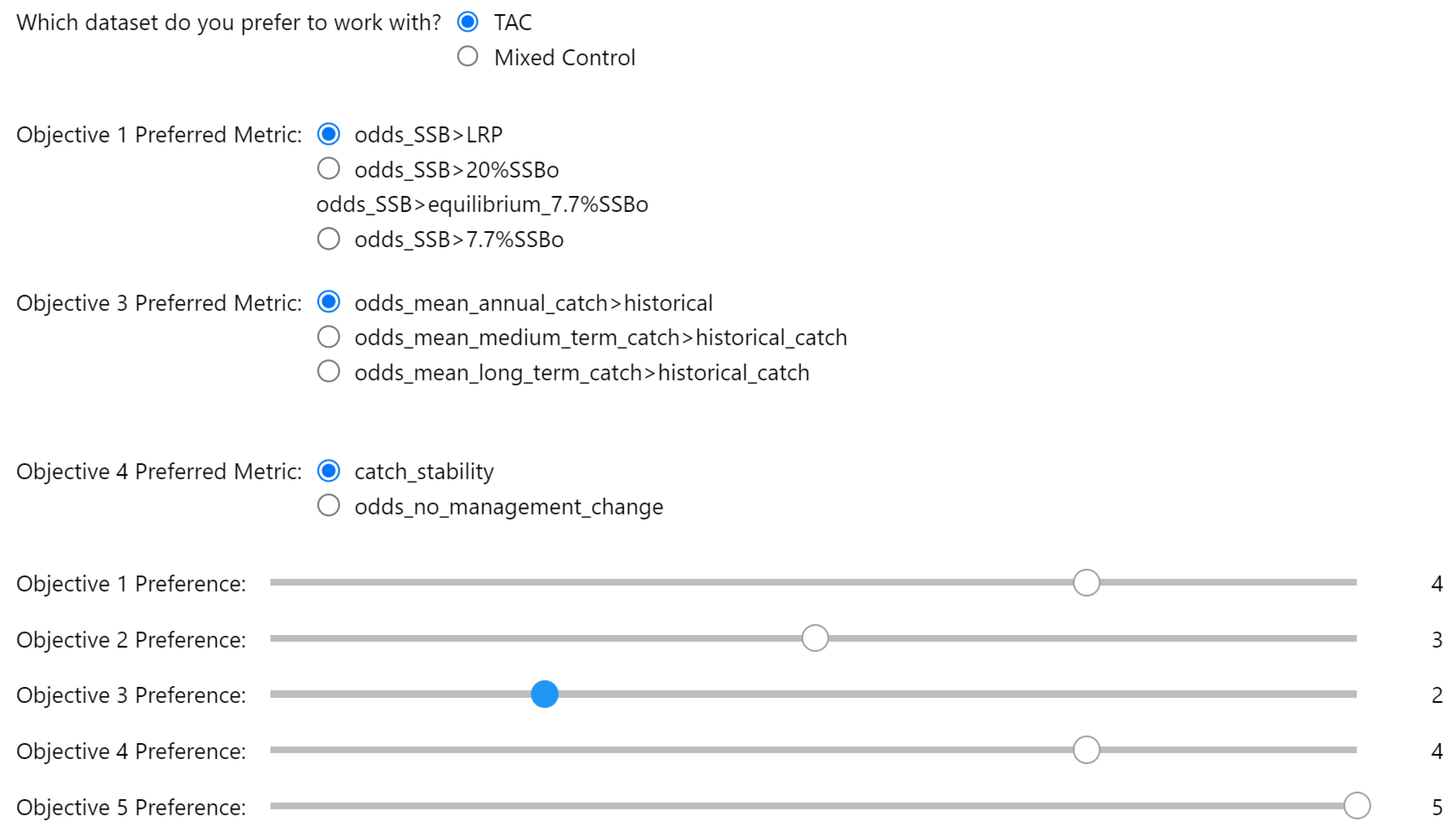
2.3. Implementation of WSM and TOPSIS with User Participatory Interface

A user participatory interface was developed to take weight inputs, generate HCR rankings, and present ranking differences. The following implementation for the NPALB dataset was inspired by the online MSE tool implementation by the Pacific Fishery Management Council [4]. Compared to swing weighting, which is more sensitive to range, direct rating better serves the research topic as it is more intuitive and creates better contrast when comparing TOPSIS to the WSM [29,30]. Under the TOPSIS and WSM interface, the user is prompted to provide direct ratings and rank their preferences on five management objectives from 1 to 5, with 5 being the most important and 1 being the least. Duplicate weights (such as a list of weights of [5, 5, 3, 3, 1]) are allowed.
Figure 3 demonstrates how users will be prompted to choose their preferred objective metric and the respective weights. Note that there is no preference selection for objectives 2 and 5 because there is only one metric for these two management objectives. The user is currently able to assign integer weights to each objective for simplicity in the comparison.
The TOPSIS score for the HCRs can be now calculated based on the users’ weights and preferences on the objectives and the performance of the HCRs on the objectives. The TOPSIS method was explicitly coded. A table that contains the TOPSIS scores, WSM scores, and the respective rankings of the HCRs was aggregated, as shown in Figure 4.
The implementation of the comparison for AMPLE datasets was conducted using a highly similar structure, only that in this scenario, the users did not need to choose which metrics they preferred to evaluate for each management objective. Rather, they are prompted to either provide weights or generate random weights for each performance metric. The WSM and TOPSIS scores and respective rankings were also computed and are graphically presented.

3. Results

In this section, the differences in HCR ranking after employing the WSM and TOPSIS and the sensitivity analysis results will be presented. Again, it should be highlighted that the results from the AMPLE dataset are hypothetical and do not reflect any species, while the ones from the NPALB dataset use actual historical data for the species.

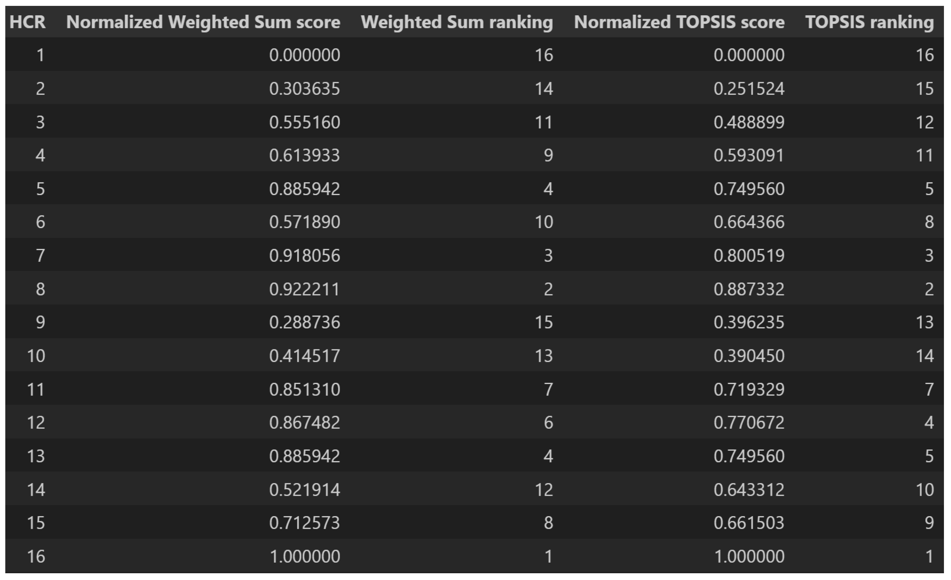
3.1. Comparison: WSM and TOPSIS

3.1.1. AMPLE Dataset

In total, 8 of the 12 graphs of the ranking differences, all using distinct sets of weights, are presented in Figure 5. The first six graphs give the scenarios where the user only focuses on one of the objectives. The other two graphs use random weights for all six objectives to simulate user inputs. The remaining four graphs are included in Appendix B for reference.
In the figures, the original HCR ranking that resulted from the WSM is on the left-hand side, and the alternative result from the TOPSIS algorithm is on the right-hand side. The connecting lines represent the change in ranking. If there is no change, the line is flat and is colored yellow; if there is a demotion or promotion in ranking, then it is symbolized by a decreasing and increasing slope colored red or green, respectively. The figures also contain the set of weights simulated for each scenario.
Some noteworthy points to be observed include the following: (1) There are some potential clusterings if grouped by the overall scales of change, which may be due to the parameter’s nature. (2) Changes in highly ranked HCRs are frequently observed, leading to different best-performing alternatives. (3) In general, for the majority of HCRs, the promotion/demotion scale is not extreme, and within the exceptions, those that experience more drastic changes are more likely to be HCRs that are promoted instead of those demoted.

3.1.2. NPALB Dataset

Three example simulations of user input using the TAC dataset and their differences in the HCR ranking results of the weighted sum method and TOPSIS are presented in Figure 6.
There are several significant patterns that could be noteworthy from Figure 6: (1) The scale of change in the HCR ranking varies with the user’s preferences. However, we observed that an HCR will not improve or drop its ranking drastically due to the switch from the WSM to TOPSIS. (2) The changes in the ranking for the high-ranking HCRs are frequently observed. (3) A significant portion of the HCRs stays where they are in terms of ranking.

3.2. Sensitivity Analysis

To reiterate, sensitivity analysis provides an evaluation of how much each component contributes to the target variable, which is, in this case, the differences between the HCR rankings generated by the WSM and TOPSIS. Since the goal of this study was to investigate the aforementioned differences, the sensitivity analysis could reveal the significance of the components in them.

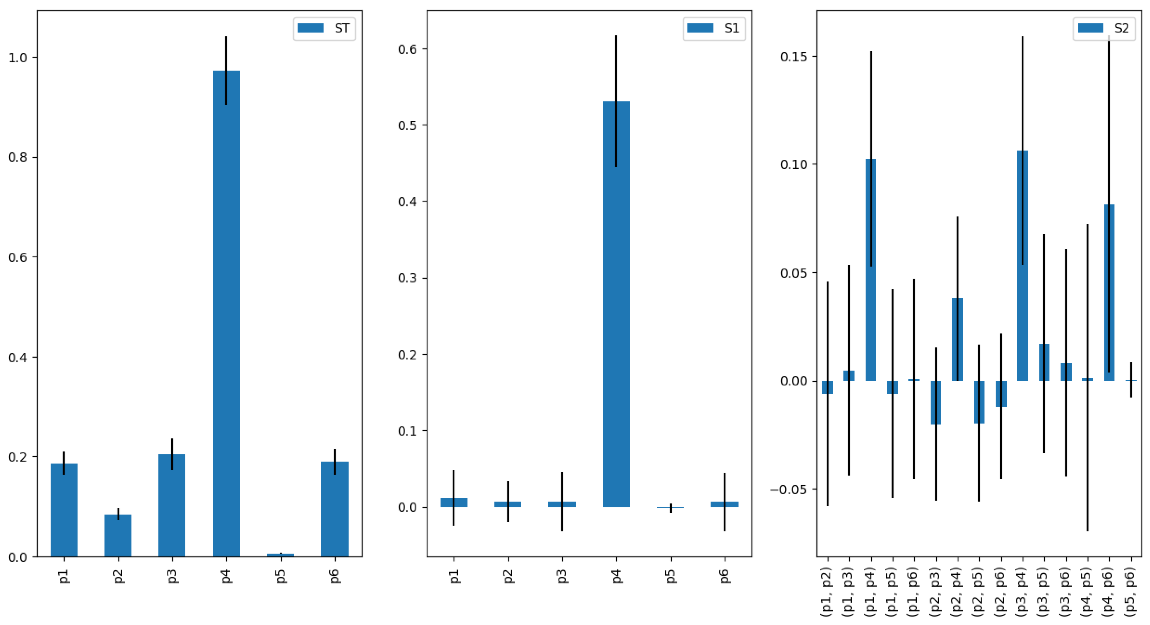
3.2.1. AMPLE Dataset

The sensitivity analysis results for the AMPLE dataset are provided in Figure 7. The p 4 component, i.e., the relative effort parameter, appears to have a significantly greater impact than other contributors, whereas the p 5 component, i.e., the catch stability parameter, contributes almost no effect on deciding the HCR rankings. It could also be observed that those with higher second-order sensitivity are the relationships connected to p 4 , potentially influenced by the very high first-order sensitivity of p 4 .

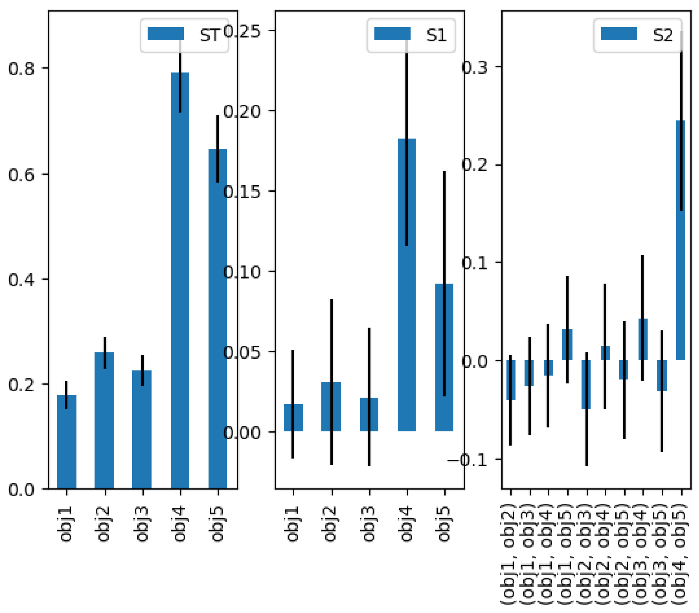
3.2.2. NPALB Dataset

As we may observe from the first-order indices in Figure 8, the total-order indices, and their similarity in distribution, objective 4 is the most influential contributor to the changes in HCR ranking, and objective 5 follows. They are much more influential on the target than objectives 1, 2, and 3 in the given NPALB dataset. The second-order indices suggest that objectives 4 and 5 are highly associated with each other with regard to their influences on the target variable.

4. Discussion

This study performed an output-based if-scenario analysis for HCR recommendations based on the MSE tools. It does not modify the existing MSE structure in its combination of the cyclical, generative iterations of biomass and fish catch predictions with a given set of HCR parameters. The lack of such contribution to the MSE system constitutes a major limitation of the decision support tool using MCDM algorithms that build directly on the performance metrics depending on the reliable evaluation of the HCRs in the previous stages. The satisfactory production of evaluative metrics is not automatic. In fact, fine-tuning the HCR thresholds and whether to include more information into the MSE process are important subjects of research value, and MSE tools themselves usually come with a large amount of potentially questionable assumptions and limitations, many of which are pre-agreed upon [1,2,3,14]. Two examples of such limitations include (1) the generalization issue due to the data-driven nature that requires long time-series, which many species simply do not have, and (2) the assumption that HCRs are carried out universally and identically in the survey regions [4].
On top of sharing all the limitations from the MSE tools, deciding on what HCRs to consider as candidates may influence TOPSIS more significantly than other potential alternatives because the TOPSIS algorithm relies heavily on the best and worst ideals for each criterion. For this reason, its sensitivity to the appropriate selection of HCRs could be heightened, and the TOPSIS algorithm could potentially be more demanding in terms of having the correct underlying datasets. This underlying assumption is not what decision makers could easily infer from the presented scores, so the risk should be identified beforehand. The consistency and robustness of TOPSIS against other potential algorithms when provided datasets with distinct distributions could be a topic for further research.
It should be recognized that there exist many algorithmic derivatives of the weighted sum method combined with other algorithms that are particularly effective for multi-objective optimization, but not in its linear form [31,32]. Due to the limitation of the study scope, as well as the popularity of the WSM in its simplest form, the algorithms were investigated as such. In essence, this study only sought to validate the theoretical advantages of TOPSIS over the WSM and to illustrate the differences in the HCR ranking outputs that imply decision support merits; whether these differences truly constitute their respective merits or not would be much harder to conclude and would require extensive field examination, surveys, and further research.
Several observations were made in the previous section for ranking differences between the WSM and TOPSIS. The shared patterns observed in both datasets include that (1) top-ranked, often the highest ranked, HCRs are frequently influenced by the switch from the WSM to TOPSIS and that (2) a majority of other HCRs experience much less significant changes in ranking. The first pattern demonstrates decision support differences (and potential values) since the policymakers are usually interested in choosing among top candidates. The second pattern actually indicates the mathematical similarities between the WSM and TOPSIS. Algorithmically, both the WSM and TOPSIS are compensatory systems, meaning that they allow alternatives to make up for their weaknesses with their strengths. Under the conditions where weights are similar or where the data have low variability, the geometric attributes of TOPSIS behave similarly to the multiplicative part of the WSM, converging their outputs. This observation matches the intuition that they are both multi-objective optimizing algorithms that seek to nuance the best alternatives, and indeed, making decisions for the best alternatives is where they differ.
Moving onto the sensitivity analysis results generated with the NPALB dataset, objectives 4 and 5 appear to be more significant contributors to the changes in the HCR rankings compared to 1, 2, and 3. Contextually, this translates to the fact that when two HCRs are compared, the focus on that changes in TAC should be gradual and that maintaining a fishing intensity at the TRP with reasonable variability is more prominent than other objectives, including a minimum SSB, an average depletion, and an average catch. Also, it could be observed that compared to other pairwise sensitivity relations, the one between objective 4 and objective 5 is outstandingly strong. This indicates that the changes in the performance of these two management objectives are highly associated with one another when an HCR is evaluated under the given framework. There could be many explanations for the current scenario: for example, HCR objectives 1, 2, and 3 are not heavily concerned because the NPALB stock is very healthy. In fact, the recent report indicates that since 2016, the fish catch, spawning biomass, and recruitment are stable [28]. In such a case, objectives 4 and 5, which focus on the limitation of policy changes, would naturally be more significant contributors, while objectives 1, 2, and 3 could potentially be more significant in fish populations that have been over-exploited. It is important to note that some objectives are not inherently or persistently more important than the other ones even if they are more significant contributors in one case or for one species in a specified time period. Establishing concrete connections to the actual fish species and its ecological and social ground could generate more insights on the decision support. On the other hand, the sensitivity analysis for the AMPLE dataset, due to the lack of context, also lacks in explainability.

5. Conclusions

This study presents TOPSIS as an alternative evaluation method for the order of recommending HCRs that are composed of essential fishery policy metrics, based on future projections in a fish population model. The demonstration of the differences between the output of the currently employed Weighted Sum Method and the alternative TOPSIS method was the main objective of the study. Based on the results, two preliminary conclusions are drawn: (1) TOPSIS overcomes significant theoretical limitations of the WSM and is more robust in the setting of fishery MSE, and the differences between the HCR rankings generated by the two methods are visible; (2) the change in ranking in higher-ranked HCRs is often observed, and this may produce realistic decision-making values.

Author Contributions

Conceptualization, J.L., Z.S., and Z.Z.; data curation, J.L.; formal analysis, J.L.; funding acquisition, Z.Z.; investigation, J.L.; methodology, J.L. and Z.Z.; project administration, Z.Z.; resources, J.L.; software, J.L.; supervision, Z.Z.; validation, J.L., Y.X., and Z.Z.; visualization, J.L.; writing—original draft, J.L.; writing—review and editing, Z.S., Y.X., and Z.Z. All authors have read and agreed to the published version of the manuscript.

Funding

This project was funded by the National Science Foundation under Grants # 2137684, # 2321069, and # 2339174.

Institutional Review Board Statement

Not applicable.

Informed Consent Statement

Not applicable.

Data Availability Statement

The performance metric data are publicly available for download using the following link.

Conflicts of Interest

The authors declare no conflicts or interest.

Abbreviations

The following abbreviations are used in this manuscript:
HCRHarvest Control Rule;
TOPSISTechnique for Order Preference by Similarity to Ideal Solution Method;
MSEManagement Strategy Evaluation;
TACTotal Allowable Catch;
TAETotal Allowable Effort;
OMOperation Model;
EMEstimation Model;
SSBSpawning Stock Biomass;
LRPLimit Reference Point;
MCDMMulti-Criteria Decision Making;
WSMWeighted Sum Method;
TRPTarget Reference Point;
ACLAnnual Catch Limit;
ABCAcceptable Biological Catch;
IATTCInter-American Tropical Tuna Commission;
ISCInternational Scientific Committee;
WCPFCWestern and Central Pacific Fisheries Commission.

Appendix A. Dataset: HCR Evaluation on AMPLE [5]

Table A1. HCRs generated with AMPLE: Column 1: number; Columns 2–5: HCR parameters; Columns 6–11: performance metrics.
HCRBlimBelbowCminCmaxProb. > LRPCatchRelative CPUERelative EffortCatch StabilityProx to TRP
10.20.65012511000.661.60.890.8
20.20.6502000.55670.332.10.880.4
30.20.6751250.8990.541.90.930.66
40.20.6752000210.048.80.850.049
50.20.8501251980.821.20.920.91
60.20.8502000.95870.481.80.880.58
70.20.8751250.991100.791.40.950.92
80.20.8752000.13470.146.30.840.17
90.250.6501251980.741.30.950.86
100.250.6502001840.511.60.910.6
110.250.6751250.99980.641.50.970.75
120.250.6752000.38520.195.50.880.22
130.250.8501251970.9110.960.93
140.250.8502001920.631.50.920.74
150.250.87512511000.851.20.980.95
160.250.8752000.81820.441.90.950.51
170.30.6501251990.761.30.940.9
180.30.6502001900.591.50.890.69
190.30.67512511000.711.40.960.83
200.30.6752000.91830.491.70.930.58
210.30.8501251970.9510.960.88
220.30.8502001960.71.40.930.82
230.30.87512511000.861.20.970.93
240.30.8752000.99870.541.60.950.63
250.40.6501251950.711.30.780.87
260.40.6502001920.641.50.530.76
270.40.67512511000.681.40.860.83
280.40.6752000.89900.581.60.770.71
290.40.85012511000.911.10.870.89
300.40.8502001950.711.30.780.86
310.40.8751251990.81.20.920.93
320.40.8752000.97990.651.50.830.79

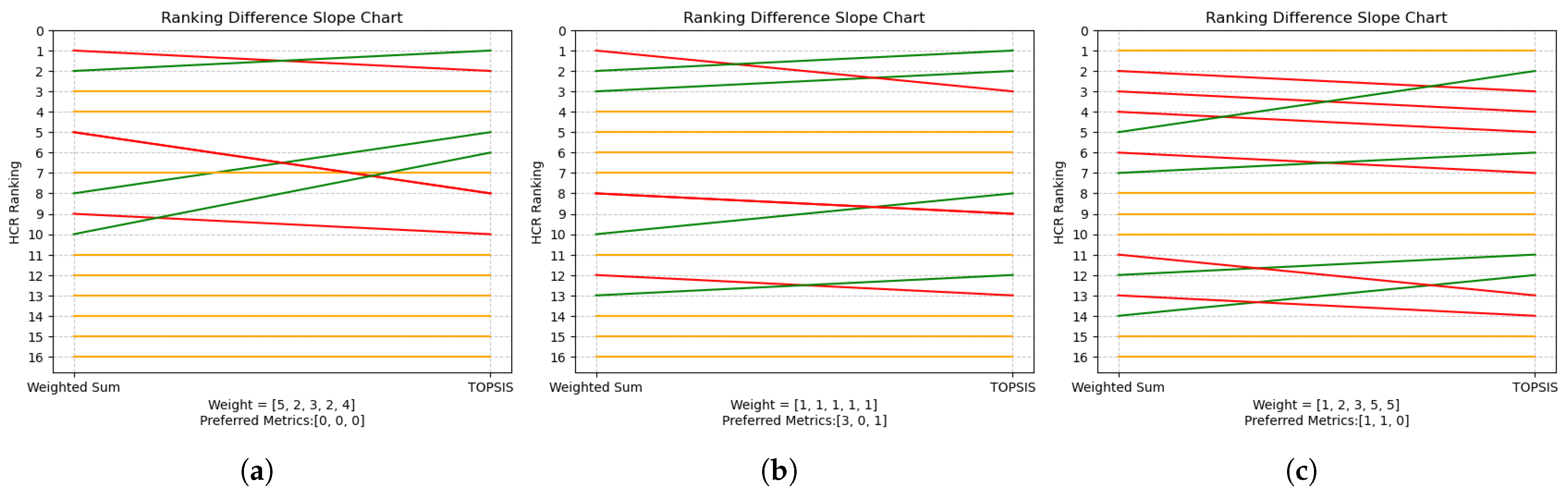
Appendix B. Graphs: Change in HCR Rankings with AMPLE Dataset

Figure A1. Movement in HCR rankings due to alternative algorithm. (ad) The change in HCR ranking for randomly generated user weights sets. (a) Random Weight Set 3, (b) Random Weight Set 4, (c) Random Weight Set 5, (d) Random Weight Set 6.
Fishes 10 00140 g0a1

Appendix C. Dataset: TAC HCR Evaluation with NPALB by ISC [4]

Table A2. HCRs in NPALB Case: Column 1: number; Columns 2–5: HCR parameters; Columns 6–9: objective 1 metrics; Column 10: objective 2 metrics; Columns 11–13: objective 3 metrics; Columns 14–15: objective 4 metrics; Column 16: objective 5 metrics.
hcrTRPLRPSSB Thre SholdFrac Tion Fodds SSB > LRPodds SSB > 20% SSBoodds SSB > 7.7% SSBoodds SSB > 7.7% SSBoDeple Tion > Minimum HistoricalAnnual Catch > HistoricalMed Term > HistoricalLong Term > HistoricalCatch StabilityNo Management Changef Target over f
1F500.20.30.250.920.920.920.990.70.630.640.680.70.770.88
2F500.140.30.250.960.920.920.980.70.620.640.680.720.770.89
3F500.080.300.980.910.920.980.70.620.640.670.750.760.89
4F500.140.20.250.960.910.920.980.70.630.650.680.780.910.88
5F500.080.200.980.910.920.980.690.650.670.710.820.910.87
6F400.140.20.250.930.870.90.970.680.640.610.730.630.871.06
7F400.080.200.970.880.90.970.680.660.630.750.660.881.05
8F400.080.1400.960.860.90.960.670.670.630.750.70.921.02
9F500.20.30.50.910.910.920.980.70.630.660.680.750.760.89
10F500.140.30.50.960.920.920.990.70.620.640.690.740.770.89
11F500.080.30.250.990.920.920.990.70.630.670.690.790.770.89
12F500.140.20.50.960.910.920.980.70.640.660.70.820.910.88
13F500.080.20.250.980.910.920.980.690.650.660.710.820.910.87
14F400.140.20.50.920.860.90.960.670.650.630.730.670.861.02
15F400.080.20.250.970.870.90.970.670.660.640.740.670.871.01
16F400.080.140.250.960.860.90.960.670.660.650.750.710.921.03

References

  1. Deroba, J.J.; Bence, J.R. A review of harvest policies: Understanding relative performance of control rules. Advances in the Analysis and Application of Harvest Policies in the Management of Fisheries. Fish. Res. 2008, 94, 210–223. [Google Scholar] [CrossRef]
  2. Free, C.M.; Mangin, T.; Wiedenmann, J.; Smith, C.; McVeigh, H.; Gaines, S.D. Harvest control rules used in US federal fisheries management and implications for climate resilience. Fish Fish. 2023, 24, 248–262. [Google Scholar] [CrossRef]
  3. Zahner, J.A.; Branch, T.A. Management strategy evaluation of harvest control rules for Pacific Herring in Prince William Sound, Alaska. ICES J. Mar. Sci. 2024, 81, 317–333. [Google Scholar] [CrossRef]
  4. International Scientific Committee for Tuna and Tuna-like Species in the North Pacific Ocean. MSE Web Tool. Available online: https://pfmc.shinyapps.io/Albacore_MSE/ (accessed on 1 November 2022).
  5. The Pacific Community (SPC). AMPLE MSE—Measuring HCR Performance. Available online: https://ofp-sam.shinyapps.io/AMPLE-measuring-performance/ (accessed on 1 February 2025).
  6. Takagi, M.; Okamura, T.; Chow, S.; Taniguchi, N. Preliminary study of albacore (Thunnus alalunga) stock differentiation inferred from microsatellite DNA analysis. Fish. Bull.-Natl. Ocean. Atmos. Adm. 2001, 99, 697–701. [Google Scholar]
  7. Ramon, D.; Bailey, K. Spawning seasonality of albacore, Thunnus alalunga, in the South Pacific Ocean. Oceanogr. Lit. Rev. 1997, 7, 752. [Google Scholar]
  8. Nikolic, N.; Morandeau, G.; Hoarau, L.; West, W.; Arrizabalaga, H.; Hoyle, S.; Nicol, S.J.; Bourjea, J.; Puech, A.; Farley, J.H.; et al. Review of albacore tuna, Thunnus alalunga, biology, fisheries and management. Rev. Fish Biol. Fish. 2017, 27, 775–810. [Google Scholar]
  9. Akayli, T.; Karakulak, F.; Oray, I.; Yardimci, R. Testes development and maturity classification of albacore (Thunnus alalunga (Bonaterre, 1788)) from the Eastern Mediterranean Sea. J. Appl. Ichthyol. 2013, 29, 901–905. [Google Scholar]
  10. Gillett, R. Tuna for Tomorrow: Information on an Important Indian Ocean Fishery Resource; Technical Report, Smartfish Working Papers, EU; Indian Ocean Commission-Smart Fish Programme: Ebène, Mauritius, 2013; 55p. [Google Scholar]
  11. NOAA. Pacific Albacore Tuna. 2023. Available online: https://www.fisheries.noaa.gov/species/pacific-albacore-tuna (accessed on 1 February 2024).
  12. Wells, R.D.; Kohin, S.; Teo, S.L.; Snodgrass, O.E.; Uosaki, K. Age and growth of North Pacific albacore (Thunnus alalunga): Implications for stock assessment. Fish. Res. 2013, 147, 55–62. [Google Scholar] [CrossRef]
  13. NOAA. West Coast Research Alliance Projects Climate Effects, Management Options for Key Species. Available online: https://www.fisheries.noaa.gov/news/west-coast-research-alliance-projects-climate-effects-management-options-key-species (accessed on 1 July 2024).
  14. ISC. Report of the North Pacific Albacore Tuna Management Strategy Evaluation. 2021. Available online: https://isc.fra.go.jp/pdf/ISC21/ISC21_ANNEX11_Report_of_the_North_Pacific_ALBACORE_MSE.pdf (accessed on 13 February 2023).
  15. NOAA. Fishery Landing Data. 2023. Available online: https://www.fisheries.noaa.gov/foss (accessed on 15 January 2025).
  16. Jacobsen, N.S.; Marshall, K.N.; Berger, A.M.; Grandin, C.; Taylor, I.G. Climate-mediated stock redistribution causes increased risk and challenges for fisheries management. ICES J. Mar. Sci. 2022, 79, 1120–1132. [Google Scholar] [CrossRef]
  17. Hwang, C.; Yoon, K. Multiple Attribute Decision Making: Methods and Applications A State-of-the-Art Survey; Springer: New York, NY, USA, 1981. [Google Scholar] [CrossRef]
  18. Behzadian, M.; Khanmohammadi Otaghsara, S.; Yazdani, M.; Ignatius, J. A state-of the-art survey of TOPSIS applications. Expert Syst. Appl. 2012, 39, 13051–13069. [Google Scholar] [CrossRef]
  19. Zhang, Z.; Demšar, U.; Rantala, J.; Virrantaus, K. A fuzzy multiple-attribute decision-making modelling for vulnerability analysis on the basis of population information for disaster management. Int. J. Geogr. Inf. Sci. 2014, 28, 1922–1939. [Google Scholar]
  20. Zhang, Z.; Hu, H.; Yin, D.; Kashem, S.; Li, R.; Cai, H.; Perkins, D.; Wang, S. A cyberGIS-enabled multi-criteria spatial decision support system: A case study on flood emergency management. In Social Sensing and Big Data Computing for Disaster Management; Routledge: Abingdon, UK, 2020; pp. 167–184. [Google Scholar]
  21. Zhang, Z.; Zou, L.; Li, W.; Albrecht, J.; Armstrong, M. Cyberinfrastructure and Intelligent Spatial Decision Support Systems. Trans. GIS 2021, 25, 1651–1653. [Google Scholar] [CrossRef]
  22. Hwang, C.L.; Lai, Y.J.; Liu, T.Y. A new approach for multiple objective decision making. Comput. Oper. Res. 1993, 20, 889–899. [Google Scholar] [CrossRef]
  23. Yoon, K. A Reconciliation Among Discrete Compromise Solutions. J. Oper. Res. Soc. 1987, 38, 277–286. [Google Scholar] [CrossRef]
  24. Zhang, Z.; Demšar, U.; Wang, S.; Virrantaus, K. A spatial fuzzy influence diagram for modelling spatial objects’ dependencies: A case study on tree-related electric outages. Int. J. Geogr. Inf. Sci. 2018, 32, 349–366. [Google Scholar]
  25. Saltelli, A.; Annoni, P. How to avoid a perfunctory sensitivity analysis. Environ. Model. Softw. 2010, 25, 1508–1517. [Google Scholar]
  26. Sobol, I. Global sensitivity indices for nonlinear mathematical models and their Monte Carlo estimates. The Second IMACS Seminar on Monte Carlo Methods. Math. Comput. Simul. 2001, 55, 271–280. [Google Scholar] [CrossRef]
  27. Scott, F. Amazing Management Procedure Exploration Device (AMPED). Version 0.2.0. 2019. Available online: https://github.com/PacificCommunity/ofp-sam-amped (accessed on 1 February 2025).
  28. ISC. Stock Assessment Report for Albacore Tuna in the North Pacific Ocean. 2023. Available online: https://apps-st.fisheries.noaa.gov/sis/docServlet?fileAction=download&fileId=9373 (accessed on 1 July 2023).
  29. Fischer, G.W. Range sensitivity of attribute weights in multiattribute value models. Organ. Behav. Hum. Decis. Process. 1995, 62, 252–266. [Google Scholar]
  30. Rezaei, J.; Arab, A.; Mehregan, M. Analyzing anchoring bias in attribute weight elicitation of SMART, Swing, and best-worst method. Int. Trans. Oper. Res. 2022, 31, 918–948. [Google Scholar]
  31. Kim, I.Y.; De Weck, O.L. Adaptive weighted-sum method for bi-objective optimization: Pareto front generation. Struct. Multidiscip. Optim. 2005, 29, 149–158. [Google Scholar]
  32. Wang, R.; Zhou, Z.; Ishibuchi, H.; Liao, T.; Zhang, T. Localized weighted sum method for many-objective optimization. IEEE Trans. Evol. Comput. 2016, 22, 3–18. [Google Scholar] [CrossRef]
Figure 1. Visualization of one potential implementation of a threshold-based HCR with the “Hockey Stick” shape. The X-axis is the biomass level, and the Y-axis is the fishing intensity or the prospective catch. The line demonstrates its boundaries for different harvesting actions. This visualization is inspired by the cited works [4,5].
Fishes 10 00140 g001
Figure 2. A visualization of how the current MSE tool evaluates HCRs.
Fishes 10 00140 g002
Figure 3. User interface for NPALB: select weights and objective preferences. The user is able to choose their preferred metrics to be evaluated for objectives 1, 3, and 4 while assigning weights to each objective. Note that the user does not need to define their preferences for objectives 2 and 5 because these two objectives have only one metric available. The blue coloring of the button on the Objective 3 Preference slide bar signifies the current user selection for weight adjustment.
Fishes 10 00140 g003
Figure 4. User interface for NPALB: summary table with scores and rankings from the WSM and TOPSIS. Notice that the information from the table is listed in ascending order for the HCR number, while the parameters are put in parallel columns to visualize the ranking differences between choosing the WSM and TOPSIS.
Fishes 10 00140 g004
Figure 5. Movement in HCR rankings due to the alternative algorithm. (af) The change in the HCR ranking when the user only focuses on one parameter, i.e., assigning a weight of 5 to one parameter and a weight of 1 to the others. (g,h) Randomly generated user weight sets. The HCRs listed here correspond to the ones listed in Appendix A. (a) Focus on Parameter 1, (b) Focus on Parameter 2, (c) Focus on Parameter 3, (d) Focus on Parameter 4, (e) Focus on Parameter 5, (f) Focus on Parameter 6, (g) Random Weight Set 1, (h) Random Weight Set 2.
Fishes 10 00140 g005
Figure 6. Movement in HCR rankings due to alternative algorithm. (a) Parameter set 1 with weights = [5, 2, 3, 2, 4] and preferred metrics = [0, 0, 0]. (b) Parameter set 1 with weights = [1, 1, 1, 1, 1] and preferred metrics = [3, 0, 1]. (c) Parameter set 1 with weights = [1, 2, 3, 5, 5] and preferred metrics = [1, 1, 0]. The weights and selection of metrics are randomly generated sets to imitate distinct user inputs with distinct interest on different aspects of the HCRs. For example, the user with the first set of weights is more concerned with objective 1, i.e., maintaining the SSB higher than the LRP, and less so on objective 2, i.e., maintaining the depletion of total biomass around the historical average depletion, where objectives 1, 2, and 4 were evaluated using their first options. The user with the second set of weights is equally concerned on every objective and chose to evaluate objectives 1, 2, and 4 with their fourth, first, and second options, respectively. The specifications of the examined NPALB HCRs are provided in Appendix C.
Fishes 10 00140 g006
Figure 7. AMPLE dataset sensitivity analysis results. S1—first-order, direct influence from variables; S2—second-order, interactions among variables; ST—total-order, combined effort from variables.
Fishes 10 00140 g007
Figure 8. NPALB Dataset sensitivity analysis results with the same definitions.
Fishes 10 00140 g008
Table 1. US fish catch for North Pacific Albacore tuna and estimated values by year.
YearFish Catch (Pound)Dollars
201025,519,78028,778,100
201124,358,19943,346,942
201230,722,10745,851,105
201328,523,37841,942,710
201427,316,22432,793,729
201524,906,96629,395,030
201623,024,22737,680,810
201716,464,15634,847,851
201815,326,87424,936,506
201916,797,24227,985,757
202015,790,67524,106,123
20217,921,17315,969,360
202216,278,85135,245,038
Disclaimer/Publisher’s Note: The statements, opinions and data contained in all publications are solely those of the individual author(s) and contributor(s) and not of MDPI and/or the editor(s). MDPI and/or the editor(s) disclaim responsibility for any injury to people or property resulting from any ideas, methods, instructions or products referred to in the content.

