1. Introduction
Integrated circuits (ICs) are the most significant raw materials for modern computing systems, yet the semiconductor industry has mostly adopted a fabless business model due to rising production costs. Such an outsourced fabrication can result in severe security and privacy issues, such as IP theft, IC overproduction, and worse, the possibility of malicious modification of the design (the hardware Trojan problem). One technique proposed to hinder some of these threats is logic locking. Logic locking is based on adding additional key inputs into a design so that the circuit is unintelligible absent a correct secret key, which is programmed post-fabrication by a trusted party.
Most locking schemes are secure against naive brute-force attacks. In 2015, the Satisfiability-Based attack (SAT attack) [
1,
2] against locking was introduced. The SAT attack is an Oracle-Guided (OG) attack in that it uses functional queries to an unlocked IC to learn the value of the secret key bits. The attack employs a modern SAT solver to search for input patterns that can exclude incorrect keys, query them on the oracle, and use the same SAT solver to find keys that satisfy the input-output relations. The runtime of the attack is a function of the number of needed queries and the solving time for each instance. Both of these values are incredibly difficult to compute for a general circuit as they reduce to hard computational problems. Running the attack to observe its runtime can take prohibitively long, especially for hard-to-deobfuscate circuits. Then, the challenge becomes: given restricted time and hardware resources, can we estimate the deobfuscation time without fully performing the SAT attack?
While there has been some research on runtime prediction of SAT instances, OG attacks require multiple SAT calls, some of which may be hard. Recent work [
3] has suggested that a Graph Convolutional Network (GCN) [
4] based solution called ICNet can be used to predict the runtime of SAT attacks. This was applied in [
3] to single circuits with varying key sizes and gate types, demonstrating that key size and gate type are features that affect SAT attack run time. However, it is not clear yet if such a GCN is truly learning the topological and functional circuit properties that are the source of deobfuscation hardness for arbitrary circuits and distinguish meaningfully between different locked circuits that are not in the immediate training dataset of the model.
This paper focuses on the above question and on the need for metrics that capture such generic deobfuscation hardness. We specifically deliver the following:
We set up a control experiment. We develop a novel synthetic circuit benchmark set of Substitution-Permutation Networks (SPN), which is the basis for the most efficient yet secure keyed-functions used today: block-ciphers. We then ask whether a GCN fully trained on traditional ISCAS benchmarks can predict the simple fact that a deep SPN is more secure than a wide SPN of the same size, to which we surprisingly discover the answer to be negative.
Motivated by block-cipher design principles, we develop a set of engineered features extracted from the circuit graph. These include various measures of depth, which are critical in SPNs, along with width. Furthermore, we propose a partitioning scheme that allows mapping the circuit to a possible SPN analog and measures cryptanalysis metrics such as differential statistics and bit propagation width. We show how simple combinations of these metrics can beat the GCN on the SPN hardness prediction task.
We take these metrics back to the non-SPN benchmark set and show that many positively and consistently correlate with runtime. This means that there is an important utility in extracting deeper engineered features for deobfuscation hardness. If not to supplant end-to-end learning, such metrics can certainly aid it.
The paper is organized as follows.
Section 2 presents backgrounds for logic locking, SAT attack, GCNs, and relevant backgrounds.
Section 4 presents the analysis of the prediction model and features.
Section 5 shows experimental results.
Section 6 draws the conclusion for the paper.
2. Background
Logic locking. Formally, a logic locking scheme is an algorithm that transforms an
n-input
m-output original circuit
to a locked circuit
by adding
l new key inputs, in a way that hides/corrupts the functionality of
absent some correct key
. The locked circuit is fabricated by the untrusted foundry, and the correct key is programmed post-fabrication. Randomly inserting key-controlled XOR/XNOR gates, lookup-tables, AND-trees/comparators, and MUX networks are among common ways to implement locking [
5].
SAT attack. An oracle-guided attack such as the SAT attack allows the attacker to query a black-box implementation of . This corresponds to purchasing a functional/unlocked IC from the market and accessing its input/outputs/scan-chain. The attack begins by forming an SAT formula . This is derived by constructing the circuit for M and then using the Tseitin transform to convert it to an SAT Conjunctive-Normal-Form (CNF) formula. Satisfying M returns a Discriminating Input Pattern (DIP) , which is queried on the oracle obtaining . The resulting input-output relation is appended to M. The process continues until the formula is no longer satisfiable at which point solving the IO-relations will return a functionally correct key .
Graph Neural Networks (GNN). Most deep learning algorithms specialize in dealing with fixed-dimensional data. Many types of data, such as social networks, chemical structures, and circuits, are graph-like in nature. Graph Neural Networks (GNN) are a class of recent machine learning models that can directly operate on graphs and perform various learning tasks. Many of these models operate by taking in an initial set of node features as the node encoding. They then iteratively apply operations on the node features and the graph’s adjacency matrix that correspond to some variant of data being passed around and accumulated in the graph nodes along edges. This is all achieved without explicitly storing the dense representation of the graph’s adjacency matrix. GNNs have been shown to be effective for both node-level and graph-level regression and classification tasks [
4]. Graph Convolutional Networks (GCNs) are a type of GNN layer that is analogous to the convolutional operation in deep neural networks.
Substitution Permutation Networks (SPN). SPNs are the basic structure used in block-ciphers.
Figure 1 demonstrates a general structure of an SPN. An SPN is often made up of several rounds, with each round consisting of a key mixing layer, and a group of substitution boxes, known as sboxes, which create the substitution layer and a permutation layer. The key mixing layer is typically a bit-wise XOR with the key vector, which means that to have a non-linear SPN, the sbox is the main source of non-linearity. The sbox is typically a look-up table, mapping its input bits to an equal or smaller number of output bits. The permutation in its simplest form performs a reversible bit shuffle. In a block-cipher, the keys for each round of the SPN are typically different and derived from a master key via key-expansion. It is not precisely known formally what kinds of sbox operations produce the most secure SPNs, but given the right substitution+permutation operation, the security of SPNs against practical attacks increases somewhat exponentially as the number of rounds increases.
3. Putting GCN-Based Deobfuscation Hardness Prediction to the Test
GCN is one of the most effective current deep learning models for detecting graph-like structures. It has multiple message-passing layers and pooling layers, akin to CNN (Convolutional Neural Network). The message-passing layers filter each node in the graph to acquire information from its neighbors with a one-hop distance, while the pooling layer reduces computational complexity. The following rule is typically used by a GCN message passing layer to update the node encoding in step
l,
:
where
is the adjacency matrix added with self-connections,
D is the degree matrix and
W is the trainable layer weight. The weight matrix which is the tunable parameter here controls the strength of this combination. This corresponds to combining the information of one node with those collected from the node’s neighbors mentioned before. As a result, a GCN model with
n layers implies it can aggregate node messages from at most
n-hop away.
For a graph-level regression task such as predicting the runtime of the SAT attack from an obfuscated circuit graph, the node-level encodings have to be combined into a single graph-level number. This aggregation step is called global pooling. The result of the global pooling can then be passed to a fixed neural network layer such as a dense layer with an activation function. For the runtime prediction/regression task this is simply a dense layer with no activation function.
Regressing this GCN on a dataset of SAT attack times with a collection of traditional benchmarks such as ISCAS will show a drop in training loss over iterations. However, here we are interested in whether the GCN in this setting is in fact learning the true source of deobfuscation hardness. To test this, we propose to test a well-trained SAT attack predictor GCN on the task of comparing the difficulty of breaking two circuits— a task that is obvious to a human engineer.
Figure 1 shows a two-round SPN.
Figure 2 shows the same two rounds of the SPN in
Figure 1 but rather than being placed back-to-back, the rounds have been placed next to one another in parallel. The parallel placement of the rounds increases the number of inputs and the number of keys in the circuit while reducing its depth. It is a well-known fact that the deeper sequential SPN is more secure than the parallel analog. If one takes the 10 rounds of AES and places them in parallel, the key and block size may expand by 10 times, yet security is all but removed. We hence ask a well-trained GCN to predict the deobfuscation difficulty of these two SPNs and compare the results, i.e., whether
. This will demonstrate whether the GCN is simply blindly counting key inputs or has gained the simple topological heuristic that deeper circuits tend to be more secure than their parallel counterparts. We describe this experiment in
Section 5 and found that unfortunately the answer is negative.
4. SPN-Motivated Features
The inability of the end-to-end GCN to learn the simple facts about the relationship between circuit structure and deobfuscation hardness calls for the development of better metrics/features. We explore some possible metrics here motivated by the SPN structure.
We first begin by exploring some traditional alternatives to the end-to-end machine learning approach. We note that in a theoretical sense, predicting the runtime of an SAT instance is a hard computational problem. If it were not, this would violate certain long-standing assumptions; however, heuristically guessing the difficulty of practical instances of SAT problems has been a topic of research in other domains besides hardware security. The authors of [
6] highlight a wide set of features, some simple to compute and some themselves requiring potentially exponential exploration. These range from variable to graph-level features, as well as some novel features, such as closeness to the Horn formula and so on.
As for locked circuit level features, an early work in logic locking proposed analyzing the key–dependency graph of the locked circuit and searching for cliques in this graph [
7]. Deriving this metric itself reduces to the NP-complete problem of finding cliques in a graph. Subsequent work has shown that such cliques can be easily achieved by simple tricks. Metrics such as hamming distance (average number of bit-flips at the output given some input difference) were used prior to the invention of the SAT attack [
5].
In this paper, given that we showcased the failure of the GCN to compare SPN structures to one another, we derive several metrics based on SPN/block-cipher long-standing design heuristics. If one can map a generic circuit to an SPN equivalent form, then one can use metrics used in the cryptography domain for decades to design better and better SPNs as correlates of deobfuscation hardness.
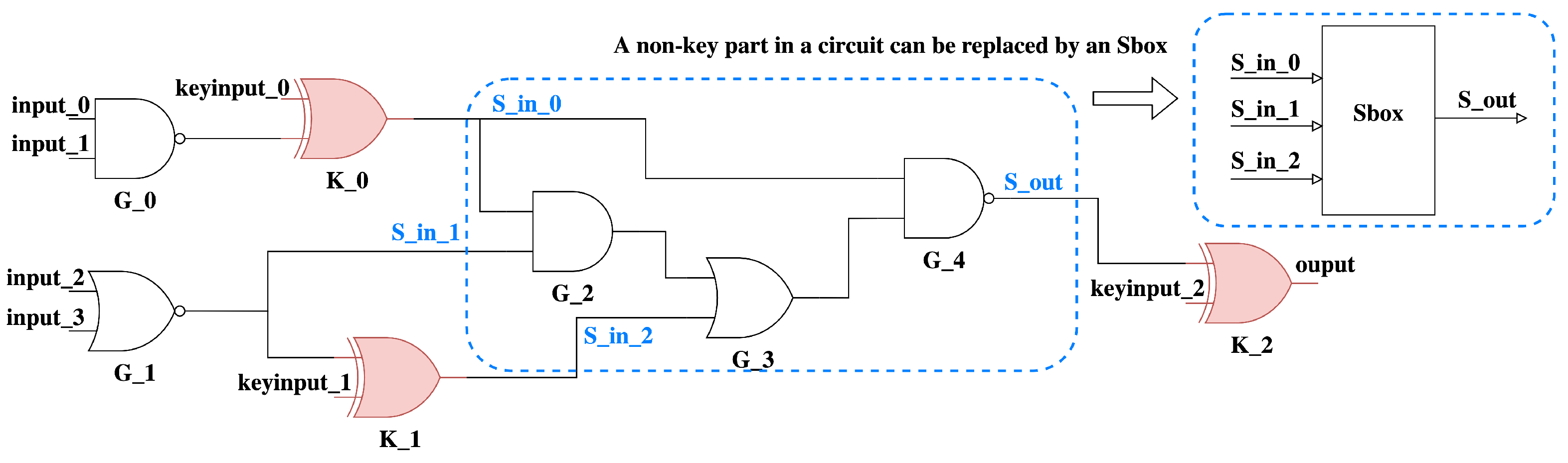
Assuming that the circuit under study is locked with XOR/XNOR insertion. Here key bits are being XOR/XNORed with internal wires. We can hence imagine that the XOR/XNOR gates are in fact part of a key-mixing layer, with the non-key gates being parts of substitution/permutation operations. While partitioning the non-key logic of the circuit into substitution/permutation blocks does not necessarily produce a unique mapping, the partitioning into key and non-key parts can be performed uniquely.
An example of this partitioning is seen in
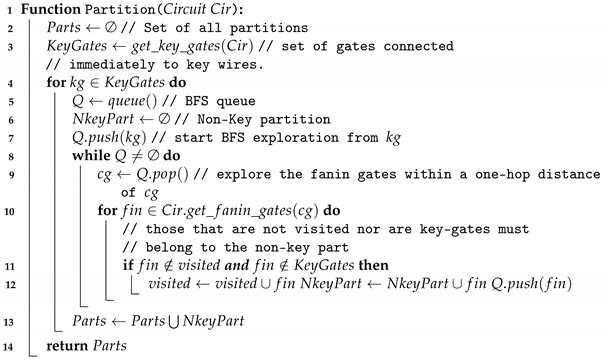
Figure 3. Here, we take the key-controlled XOR/XNOR gates as key-parts. The remaining logic is then in the form of at least one connected non-key part. Algorithm 1 shows the pseudo-code for this partitioning.
The algorithm starts by from the set of all key gates immediately connected to the key input set Keys (line 3). For each key gate in this set, we perform a backward breadth-first-search (BFS) until we reach other key gates or primary inputs. The logic explored as part of this BFS forms a new non-key part (NkeyPart). All circuit partitions (Parts) will be completed once the aforementioned procedure has been applied to all keys in Keys (line 13). We record these different partitions, which allow us to then compute a set of SPN-motivated features listed herein:
Non-key Part Structural Statistics: this includes structural information about the non-key parts. This is primarily, the average number of inputs, outputs, and gates.
Number of Active Non-key Parts: the average number of “active” non-key parts when passing a signal randomly from one of circuits’ input to an output. This is derived from the important notion of active-sboxes in block-cipher design. Given a change in some input bit, the change will propagate through the SPN touching many sboxes. The sboxes touched during this propagation are called active sboxes. The difficulty of differential cryptanalysis is directly tied to the number of active sboxes. This metric shows a surprising consistently high correlation with SAT attack time.
Non-Key Part Differential Statistics: the average output flip rate when randomly flipping a bit in non-key parts. This is derived also from differential cryptanalysis, in which changes in the input of some sbox will produce changes at its output. The closer the change at the output is to half of all bits, the more propagation there is in the circuit. Furthermore, changes in the input that produce highly-likely/impossible changes at the output can facilitate differential cryptanalysis.
| Algorithm 1: Circuit Partitioning |
![Cryptography 06 00060 i001]() |
Note that while we only explore these metrics in this paper, there is a dearth of other SPN-related metrics that can be explored which we aim to study in our future work. Examples are the nonlinearity of each non-key part, the BDD (Binary Decision Diagram) size of each non-key part, and so on.
In [
8], it was shown that the original circuit itself can have a huge impact on deobfuscation hardness. One can think of AES itself as a deep and complex original circuit that is locked by simply inserting key-mixing XOR gates and the original circuit (which includes the sboxes and AES permutation) is doing the heavy-lifting for security. The above metrics by focusing on non-key parts capture aspects of the original circuit that relate to security.
5. Experiments
We now present our experimentation. All experiments are carried out on an AMD EPYC dual-CPU 128-core, 256GB server running Ubuntu with the neos C++ SAT attack tool, which uses Glucose as its SAT solver. We use spektral [
9] for graph machine learning, and sklearn for traditional ML techniques.
5.1. Training Datasets
We generate a set of datasets that help us determine the transfer-learning ability of the GCN. Hence, we propose and build 4 datasets containing either benchmark circuits locked with the same key size or varying key sizes or datasets comprised of sequential and parallel SPNs. The goal is to train the GCN model on one dataset and evaluate it on another. Successful transfer-learning (generalization) here will be captured by a model being trained on non-SPN circuits being able to differentiate the hardness of parallel versus sequential SPNs.
SPN Generation. We generate a novel training and evaluation dataset consisting of sequential and parallel SPN circuits. The SPN circuits are constructed using a Python script. The SPN sboxes are generated as random truth tables that are synthesized to gates using ABC. The truth-table generation is repeated several times and disconnected or highly skewed SPNs are discarded. Each time an SPN is generated the sboxes are each assigned new random truth tables.
Each SPN is parameterized (and named) according to the following:
: type of SPN structure (sequential/parallel).
p: number of parallel rounds.
n: number of sboxes in each round.
l: length for an sbox. i.e., number of inputs/outputs to each sbox.
r: SPN round number (number of sequential rounds).
As such,
Figure 1 can be labeled as
while
Figure 2 may be named as
. This principle is applied to all datasets in our paper that follow.
Our traditional circuit datasets consist of benchmark circuits locked with XOR/XNOR random insertion locking. Deobfuscation times are extracted from the exact SAT attack algorithm. We average the runtime of the SAT attack across a few runs to obtain a more accurate reading. We develop four different datasets in total, a more detailed description is as follows:
Dataset_1. We first select a set of benchmarks from ISCAS-85, ISCAS-89, and ITC-99 benchmarks, respectively, with diverse depth/width statistics to form a benchmark set (c432, c499, c880, c1355, c1980, c2670, c3540, c5315, s832, s953, s1196, s1238, s1488, s1494, s3271, s5378, b04, b07, b11, b12, b13, b14). Since some of these benchmark circuits are sequential, we convert them to combinational by removing flip-flops and replacing them with primary input/output pairs. Then, each circuit in the dataset is locked using XOR/XNOR locking with 64 key bits. The locking is repeated 100 times with different random seeds that results in the XOR/XNOR key-gates being inserted in different locations. These circuits have the same key size as the evaluated SPN datasets that will be introduced later. This dataset contains circuits.
Dataset_2. This dataset is comprised of a subset of the above benchmark circuits that are difficult to break for the SAT attack. The dataset is built by adjusting key sizes from 1 to 700 for the , , and 1 to 500 for the benchmark circuits ( with more than 500 key bits was not deobfuscatable with our SAT attack). The locking is repeated 10 times for each key size. This leads to a total of 19,000 locked circuits.
Dataset_3. This dataset is derived by taking each circuit in the benchmark set in Dataset_1 (minus the benchmark due to its size and deobfuscation time) and locking it with XOR/XNOR with the key size ranging from 1 to 200. The locking is repeated 5 times with different key gate locations. This leads to 21,000 locked circuits.
Dataset_4. This is a unique and novel dataset that solely comprises SPN circuits. This is built by constructing SPNs with the following parameters. The number of sboxes in each round is for different sbox number (), sbox length (), and number of rounds (). Each SPN is regenerated 20 times. This leads to a total of SPN circuits.
5.2. Evaluation Datasets
We generate a specific SPN dataset for evaluation (evaluating transfer learning ability). These are generated correspondingly so that they will produce pairs of sequential versus parallel SPNs having roughly the same number of gates but different topologies (see
Table 1). The goal is to see if a model trained on another dataset can detect that deeper SPNs are more secure when the number of gates and keys is the same within this evaluation dataset.
5.3. GCN Evaluation Results
We use the ICNet technique to train the GCN model with three input features: key gate mask (set to 1 for key gate, else 0), gate type, and the circuit’s sparse adjacency matrix. The model has three layers and is trained until it converges using the ADAM optimizer with the MSE loss criterion. To test the model’s performance under various conditions, we train it on four training datasets established in
Section 5.1 and make predictions on the SPN comparison evaluation datasets developed in
Section 5.2.
The average SAT attack run time for this dataset is represented by the real value in
Table 2 (the real value of 1800 in the
and
circuits simply denotes an SAT attack time-out). We can conclude the following from real values: (1) Whether the SPN structure is sequential or parallel, the SAT attack execution time grows non-linearly with the rise in-depth; (2) SPNs with longer sbox lengths but the same depth take longer to attack than smaller ones, regardless of whether they are sequential or parallel, e.g.,
, it is well established in cryptography that larger sboxes are better; (3) The sequential SPN should be much harder to attack than its corresponding parallel SPN, e.g.,
. These findings are consistent with block-cipher design principles. As a result, if GCN can truly estimate a circuit’s run time or security, the outcomes of its prediction should at the very least fulfill the aforementioned observations.
However,
Table 2 shows that even if we train the GCN on our prepared four types of datasets, including normal and time-out situations the GCN fails at this comparison task. The evaluation results indicate that the trained GCN can only estimate the SAT attack time at a linear rate as the circuit size grows. Even when training on
, which is developed with only SPNs using random parameters, predictions on evaluation datasets still do not perform well. The GCN expects the parallel SPNs in some cases to be even more secure than their sequential counterpart.
5.4. SPN-Motivated Metrics
We then evaluated our SPN-motivated metrics from
Section 4 on the same dataset. We ensure that our model was trained on the same training datasets as GCN and tested on the same evaluation datasets. First, we leverage our training datasets to assess the correlation between our SPN-motivated features and SAT attack time to see whether our metrics are effective. As seen in
Table 3, the average signal walk depth and max active non-key portions, two proposed metrics directly derived from SPN structures have high correlation coefficients and are both positively proportional to all training datasets, indicating that these two metrics in addition to their theoretical relation to long-standing block-cipher design principles are consistent predictors of deobfuscation hardness for locked circuits. In the last column of
Table 3, we put the average of correlations to demonstrate the metrics performance among four datasets. We picked two metrics that had interestingly high correlations with the SAT attack time and plot their scatter map in
Figure 4.
Figure 5 shows scatter plots and correlation lines for high-correlating metrics in the SPN dataset (dataset_4).
Then, we pass these SPN-like metrics as feature vectors to various ML models. Since these proposed metrics form fixed-size vectors, we choose to fit them using several popular regression models, which include Linear Regression (LR), LASSO, Support Vector Machine (SVM), Multiperception (MLP), Ridge Regression (RR), Elastic Net(EN), Theil–Sen Regression (TS), and Random Forest (RF). We create input vectors from four training datasets, train them on the aforesaid regression models, and then use these trained models to predict evaluation datasets.
Table 4 shows the most accurate prediction data for each regression model.
We can deduce from these findings that most regression models outperform the GCN. All regression models have non-linearity that matches the real data and most models can discover that sequential SPNs are more secure than their parallel counterparts.
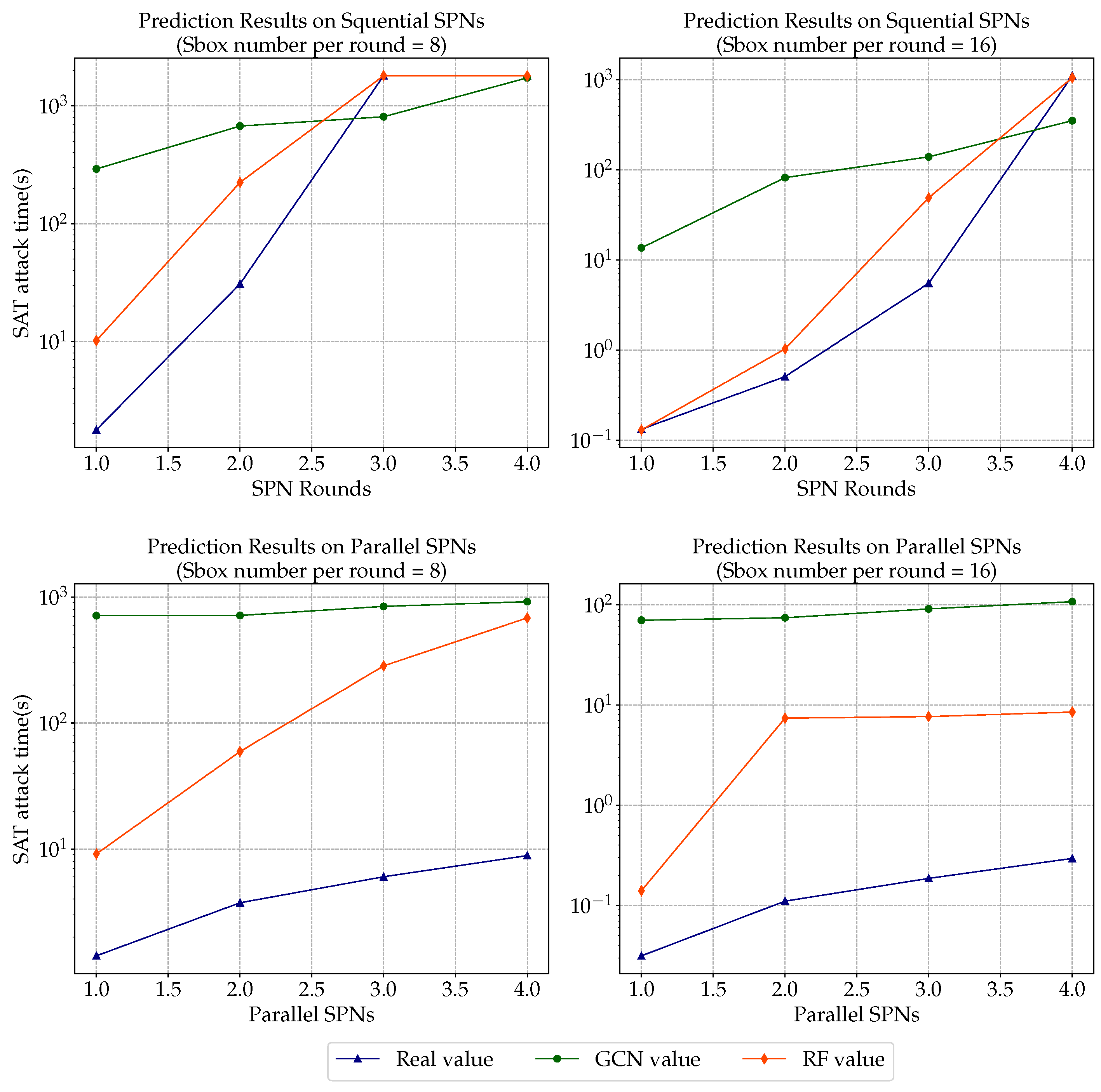
Figure 6 shows the comparison results of sequential/parallel SPNs with sbox number of four and eight accordingly. The log values of SAT attack time are shown on Y axis, while the SPN rounds/parallels are shown on the X axis. RF regression estimates all clearly reflect a similar trend as the real non-linear data while the GCN prediction does not and overestimates the parallel SPN attack time.
6. Conclusions
In this paper, we demonstrated that GCN-based SAT attack runtime prediction does not seem to be able to capture simple facts about deobfuscation hardness, such as the fact that a deeper SPN is more secure than a parallel one. We proposed a set of alternative metrics derived from SPN design principles and demonstrated their superior ability in capturing circuit complexity. Most of the regression models have shown non-linearity that matches the real data and the majority of the models tested can discover that sequential SPNs are more secure than their parallel counterparts. Among these models, random forest regression produces the most accurate results (as measured in distance from predicted to real values). We leave a deeper analysis of these metrics and the application of the above approach to non-XOR/XNOR locking schemes to future work.


