Dynamic Scaling Pollard’s P-1 Algorithm

Abstract

The integer factorization problem is a hard problem in classical. Let $N=PQ$, where P and Q are large primes. Pollard’s P-1 Algorithm is an efficient integer factorization algorithm while all the prime factors of $P-1$ are small. However, the previous variants of Pollard’s P-1 algorithms require a strict bound on the prime factors, and the running time depends on the bound instead of the actual size of prime factors, which is undesirable. This paper firstly designs a dynamic scaling version of Pollard’s P-1 Algorithm (abbreviate as $\mathsf{DSP}$) to solve this problem and also accelerate the algorithm’s efficiency by applying a fast multiplication method to it. Additionally, $\mathsf{DSP}$ saves the cost in computing the product of prime factors with high enough exponent by repeatedly using product of primes with low exponent. We also give the complexity analysis for our proposed algorithm and the latest published variant of Pollard’s P-1 Algorithm named IPP1 (Kritsanapong Somsuk, Symmetry). Moreover, we give a theoretical comparison between IPP1 and our algorithm. In particular, we show that our algorithm costs less than IPP1 in more than 95% while in IPP1 the bound of prime factors of P-1 is set to at least 64. Additionally, we also test several instances in factoring 1024-bit integers $N=PQ$ in experiment. We firstly construct the $P-1$ as a product of several randomly generated 30-bit numbers to ensure its solvability by the Pollard’s P-1 Algorithm, then test four variants of Pollard’s P-1 Algorithm. The experimental result shows that our algorithm is most efficient among them. Its efficiency improvement performs more apparently while the exponent of a prime factor in $P-1$ is large. In factoring 1024-bit integer, our algorithm solves it nearly 23.5 times faster than IPP1, 16.4 times faster than the Original Pollard’s P-1 Algorithm (J. M. Pollard, MPCPS), 35.6 times faster than the trivial Pollard’s P-1 Algorithm (D. Bishop, Introduction to cryptography with Java applets).

1. Introduction

The security of RSA [1] relies heavily on the computational difficulty of integer factorization. While general-purpose algorithms like the number field sieve (NFS) [2] exist, special-purpose methods are often more efficient for specific moduli. Notably, when a prime factor P of the RSA modulus $N=PQ$ has a “smooth” $P-1$ (i.e., consisting entirely of small prime factors), Pollard’s P-1 algorithm [3] is frequently employed. Based on Fermat’s Little Theorem [4] (i.e., ${\left[a^{P-1}\right]}_P\equiv 1$), the algorithm iteratively evaluates $gcd({[a^z-1]}_N,N)$ for a chosen base a (e.g., $a=2$), where the exponent z is constructed from all small primes up to a predefined smoothness bound B. If z is a multiple of $P-1$, we have $gcd({[a^z-1]}_N,N)=P$, thereby factoring N. However, its running time depends entirely on the largest prime factor of $P-1$, reaching a worst-case complexity of $O\left(P\right)$.

Several variants have attempted to optimize this process. A trivial version proposed by Bishop [5] iteratively tests exponent factorials (i.e., let $z=x!$ for an increasing integer x). While effective in theory, evaluating $x!$ heavily over-computes the necessary prime powers, resulting in massive inefficiency. More recently, Somsuk [6] proposed $\mathsf{I}\mathsf{P}\mathsf{P}\mathsf{1}$, which first computes the product of all primes up to a smoothness bound B (i.e., $y={\prod }_{p_i\le B}{p}_i$) and performs modular exponentiation up to $z=y^{u_{\max }}$, where $u_{\max }$ is a given upper bound on the exponents. However, $\mathsf{I}\mathsf{P}\mathsf{P}\mathsf{1}$ becomes highly inefficient if even a single prime factor of $P-1$ possesses a large exponent. Furthermore, both the original algorithm and $\mathsf{I}\mathsf{P}\mathsf{P}\mathsf{1}$ require a predefined smoothness bound B. Choosing an optimal B beforehand is practically difficult: an overly small B guarantees failure, while an overly large B wastes significant computational time.

1.1. Our Contributions

To overcome the limitations of prior methods, this paper proposes novel algorithmic improvements. The remainder of the paper is organized to detail these contributions as follows. Section 2 introduces the basic notations and preliminaries. In Section 3, we present our primary contribution, the Dynamic Scaling Pollard’s P-1 algorithm ($\mathsf{DSP}$) (Section 3.1). By employing a dynamic traversal order, $\mathsf{DSP}$ systematically enumerates prime factors and their exponents without relying on a predetermined smoothness bound. This progressive scaling and continuous reuse of prior prime products drastically reduce redundant modular exponentiations while ensuring full coverage of potential prime factors. This section subsequently provides formal cost estimators and theoretical complexity analyses for both $\mathsf{DSP}$ and $\mathsf{I}\mathsf{P}\mathsf{P}\mathsf{1}$ (Section 3.3). Furthermore, to efficiently evaluate the massive prime products required during execution, Section 4.1 introduces a novel Fast Multiplication (FM) method. We provide theoretical cost estimators and complexity analyses for both FM and the normal multiplication (NM) method (Section 4.2). A comprehensive theoretical and experimental comparison (Section 4.3) confirms the necessity of FM, demonstrating that NM incurs a time overhead ${\displaystyle \frac{2^{n+1}}{n^2}}$ times higher than our FM approach. To substantiate our approach, Section 5 conducts a detailed theoretical cost analysis and an empirical experimental comparison among four implemented variants of Pollard’s P-1 algorithm. We provide a comprehensive complexity analysis proving that $\mathsf{DSP}$ achieves strictly lower computational costs than the state-of-the-art $\mathsf{I}\mathsf{P}\mathsf{P}\mathsf{1}$ algorithm in over 95% of cases (provided $B>64$). We implemented and evaluated $\mathsf{DSP}$ alongside three prior variants on 1024-bit moduli (https://github.com/Summwer/expemeriment_of_pollardpm1, accessed on 1 August 2026). The experimental results robustly validate our theoretical estimators and highlight $\mathsf{DSP}$’s superiority when prime factors have high exponents (see Figure 1). Specifically, $\mathsf{DSP}$ operates 23.5×, 16.4×, and 35.6× faster than $\mathsf{I}\mathsf{P}\mathsf{P}\mathsf{1}$ [6], the original algorithm [3], and the trivial variant [5], respectively.

1.2. Technical Overview

1.2.1. Dynamic Scaling Pollards P-1 Algorithm

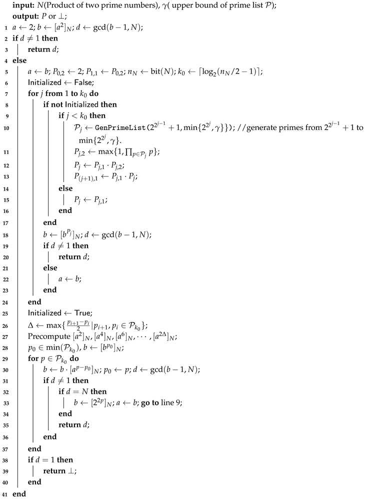
$\mathsf{DSP}$ (Algorithm 4) dynamically constructs the target exponent by partitioning prime candidates into disjoint intervals ${\mathcal{P}}_j=\left\{p\in (2^{2^{j-1}},2^{2^j}]\mid p\mathrm{is}\mathrm{prime}\right\}$. For $1\le j<k_0$ (initialized with $P_{1,1}=2$), it computes $P_{j,2}={\prod }_{p\in {\mathcal{P}}_j}p$ and recursively generates the exponent $P_j=P_{j,1}{P}_{j,2}$, updating $P_{j+1,1}=P_{j,1}{P}_j$. This yields $P_j=P_{j,2}·{\prod }_{i=0}^{j-1}{P}_{i,2}^{2^{j-i-1}}$, efficiently raising smaller primes to exponentially growing powers. By computing $b\leftarrow {\left[b^{P_j}\right]}_N$, $\mathsf{DSP}$ minimizes redundant modular exponentiations through the systematic reuse of earlier products. For the final subset ${\mathcal{P}}_{k_0}$, where any prime exponent is at most 1, $\mathsf{DSP}$ bypasses deep recursion and finishes purely via shift modular exponentiation.

1.2.2. Fast Multiplication (FM)

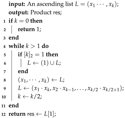
Furthermore, to efficiently evaluate massive products without introducing intolerable computational bottlenecks, we integrate our FM method. Let $L=(x_1,\cdots ,x_k)$ be an ascending list of integers defined in Section 2. Unlike NM, which computes the product linearly and accumulates unbalanced bit-lengths, FM employs a symmetric divide-and-conquer strategy. In each iteration, FM generates a new, halved sequence by pairing and multiplying elements from opposite ends, i.e., $L\leftarrow (x_1·x_k,x_2·x_{k-1},\dots ,x_{k/2}·x_{k/2+1}).$ Repeat until only a single element remains. FM ensures that intermediate 1556 products maintain strictly balanced bit-lengths at each depth of the multiplication tree. This hierarchical reduction drastically minimizes the overall asymptotic bit-complexity.

2. Preliminaries

2.1. Notations and Basic Definitions

Let $\mathbb{Z}$ denote the set of integers. For a positive integer Y, we denote the reduction of $X\left(\right(modY\left)\right)$ by ${\left[X\right]}_Y$ (i.e., $0\le {\left[X\right]}_Y<Y$). Let $N=PQ$ be an RSA modulus, where P and Q are two large distinct primes. Denote $n_N=\lfloor {log}_{2}N\rfloor +1$ as the bit-length of the modulus N. Recovering P and Q given N is known as the Integer Factorization Problem($\mathsf{IFP}$). To ensure the hardness of the $\mathsf{IFP}$ in cryptographic applications, P and Q are typically required to be of approximately equal bit-length. Under this condition, when P and Q are sufficiently large, no classical polynomial-time algorithm is currently known to solve the $\mathsf{IFP}$. Let $\varphi \left(N\right)=(P-1)(Q-1)$ denote Euler’s totient function. To facilitate our subsequent complexity analysis, we recall the Prime Number Theorem [7]: the prime-counting function $\pi \left(x\right)$, which denotes the number of primes less than or equal to x, satisfies $\pi \left(x\right)\sim {\displaystyle \frac{x}{lnx}}$.

Although the $\mathsf{IFP}$ is generally hard, special-purpose factoring algorithms (such as Pollard’s P-1) can efficiently factor N if the prime factors possess specific algebraic weaknesses. The most prominent weakness exploited by these algorithms is the smoothness of $P-1$. Formally, this property is defined as follows:

Definition 1

(B-Smooth Number). A B-smooth number is a positive integer whose prime factors are all less than or equal to B.

Following standard cryptographic settings, we assume the prime factors P and Q have a balanced bit-length $n_N/2$. Let $k_0=\lceil {log}_2(n_N/2-1)\rceil$. To ensure that the prime Q is strictly resistant to our algorithm, we assume that the largest prime factor of $Q-1$ strictly exceeds $2^{2^{k_0-1}}$.

To formally characterize the vulnerability of the prime factor P, we first consider its odd part $P_{\mathrm{div}}=(P-1)/2$, since $P-1$ is inherently even. Let $p_k$ denote the k-th prime number globally. Let $\gamma$ be the input smoothness bound (which defaults to the theoretical maximum $2^{n_N/2-1}$). We define $\mathcal{P}=\{p\in (0,\gamma ]\mid p\mathrm{is}\mathrm{prime}\}=\{p_1,p_2,\dots ,p_t\}$ as the complete list of consecutive primes up to $\gamma$, where $p_k$ denotes the k-th prime globally. Assuming $P_{\mathrm{div}}$ is $\gamma$-smooth, we let $u_i\ge 0$ denote the actual exponent of any prime candidate $p_i\in \mathcal{P}$ in its factorization. We can express this prime factorization compactly as $P_{\mathrm{div}}={\prod }_{i=1}^s{p}_{{\sigma }_i}^{u_{{\sigma }_i}}$. Here, $u_{{\sigma }_i}\ge 1$ denotes the actual exponent of the prime factor $p_{{\sigma }_i}$, and the indices satisfy $1\le {\sigma }_1<{\sigma }_2<\cdots <{\sigma }_s\le t$ (where $t=\left|\mathcal{P}\right|$). Define $e_i\in {\mathbb{Z}}^{+}$ as the explicit upper bound of this exponent, computed as $e_i=\lfloor {\displaystyle \frac{n_N/2-1}{{log}_2{p}_i}}\rfloor$. Since $P_{\mathrm{div}}<2^{n_N/2-1}$, this naturally guarantees $e_i\ge \lfloor {log}_{p_i}{P}_{\mathrm{div}}\rfloor \ge u_i$. Define the maximum actual exponent as $u_{max}={max}_{1\le i\le s}{u}_{{\sigma }_i}$, and the largest prime power factor as $R={max}_{1\le i\le s}{p}_{{\sigma }_i}^{u_{{\sigma }_i}}=p_{{\sigma }_{\max }}^{u_{{\sigma }_{\max }}}$, where ${\sigma }_{\max }\in [1,s]$ is the index achieving this maximum. For any positive integer z, let $\mathrm{bit}\left(z\right)=\lfloor {log}_{2}z\rfloor +1$ denote its bit-length. For each prime $p_i\in \mathcal{P}$, let $n_i=\mathrm{bit}\left(p_i\right)$ denote its specific bit-length. Finally, to align with our dynamic scaling strategy, we partition $\mathcal{P}$ into $k_0$ disjoint subsets, explicitly bounded by $\gamma$, denoted as ${\mathcal{P}}_j=\{p\in \mathcal{P}\mid 2^{2^{j-1}}<p\le min(\gamma ,2^{2^j})\}$ for $j=1,2,\dots ,k_0$. Let $L(p,n_1,n_2)$ be an ascending list of integers where each element $x\in [2^{n_1},2^{n_2})\cap \mathbb{Z}$ is selected independently with probability $p\in (0,1]$. For brevity, we denote this list as L, and define $L(p,n):=L(p,0,n)$.

Lemma 1.

The expected structural bit-size of the product of all elements in $L(p,n_1,n_2)$ is

$${\mathrm{bit}}_{\mathrm{LM}}(p,n_1,n_2)=p\left[2^{n_2}(n_2-1)-2^{n_1}(n_1-1)\right].$$

If $(p,n_1,n_2)=\left({\displaystyle \frac{1}{nln2}},0,n\right)$, we can obtain that ${\mathrm{bit}}_{\mathrm{LMP}}\left(n\right):={\mathrm{bit}}_{\mathrm{LM}}\left({\displaystyle \frac{1}{nln2}},0,n\right)={\displaystyle \frac{(n-1)2^n+1}{nln2}}$.

Proof. 

Let $I_x\in \{0,1\}$ be the indicator variable for $x\in L$, with expectation $\mathbb{E}\left[I_x\right]=p$. In practical arbitrary-precision arithmetic, the upper bound of the bit-size of a product is exactly the sum of the discrete bit-lengths of all operands. For any integer $x\in [2^{k-1},2^k-1]$, its exact bit-length is k.

Given that the elements in list L are bounded in the range $[2^{n_1},2^{n_2}-1]$, this range can be partitioned into subsets of exactly k-bit integers for $n_1+1\le k\le n_2$. The amount of k-bit positive integers in each subset is $2^k-2^{k-1}=2^{k-1}$.

By linearity of expectation, the expected total structural bit-length is:

$$\mathbb{E}\left[\sum _{x\in \Omega }{I}_x·\mathrm{length}\left(x\right)\right]=p{\displaystyle \sum _{k=n_1+1}^{n_2}}k·2^{k-1}.$$

Using the arithmetico-geometric sequence summation formula ${\sum }_{k=1}^{N}k{2}^{k-1}=(N-1)2^N+1$, we evaluate the bounded sum:

$$\begin{array}{cc}\hfill {\displaystyle \sum _{k=n_1+1}^{n_2}}k{2}^{k-1}& =\left[(n_2-1)2^{n_2}+1\right]-\left[(n_1-1)2^{n_1}+1\right]\hfill \\ \hfill & =2^{n_2}(n_2-1)-2^{n_1}(n_1-1).\hfill \end{array}$$

Substituting this back yields ${\mathrm{bit}}_{\mathrm{LM}}(p,n_1,n_2)=p\left[2^{n_2}(n_2-1)-2^{n_1}(n_1-1)\right]$.    □

Having established the expected bit-size of the prime products, we proceed to analyze the cumulative computational overhead of our dynamic strategy across multiple iterations. If we model the scale of the operand at the i-th iteration as a linear progression $Ai+B$, evaluating the total cost inherently involves summations of the form $\sum (Ai+B)log(Ai+B)$. By approximating this discrete summation with continuous integration, we deduce the following asymptotic bound:

Lemma 2.

$$\begin{array}{cc}\hfill & {\displaystyle \sum _{i=1}^n}(Ai+B)log(Ai+B))\hfill \\ \hfill \approx & \left({\displaystyle \frac{1}{2}}A{n}^2+Bn+{\displaystyle \frac{B^2}{A}}\right)·log(An+B)-\left({\displaystyle \frac{1}{2}}A+B-{\displaystyle \frac{B^2}{A}}\right)log(A+B)\hfill \\ \hfill & -{\displaystyle \frac{loge}{4A}}{(An+B)}^2+{\displaystyle \frac{loge}{4A}}{(A+B)}^2\hfill \end{array}$$

(1)

Proof. 

${\sum }_{i=1}^n(Ai+B)log(Ai+B)\approx {\int }_1^n(Ax+B)log(Ax+B)dx$.

$$\begin{array}{cc}\hfill & {\int }_1^n(Ax+B)log(Ax+B)dx={\int }_1^{n}log(Ax+B)d\left({\displaystyle \frac{1}{2}}A{x}^2+Bx\right)\hfill \\ \hfill =& {\left.\left({\displaystyle \frac{1}{2}}A{x}^2+Bx\right)·log(Ax+B)\right|}_1^n-{\int }_1^n\left({\displaystyle \frac{1}{2}}A{x}^2+Bx\right)dlog(Ax+B)\hfill \\ \hfill =& \left({\displaystyle \frac{1}{2}}A{n}^2+Bn\right)·log(An+B)-\left({\displaystyle \frac{1}{2}}A+B\right)log(A+B)\hfill \\ \hfill & -{\int }_1^n\left({\displaystyle \frac{1}{2}}A{x}^2+Bx\right)·{\displaystyle \frac{loge}{Ax+B}}d(Ax+B)\hfill \\ \hfill \stackrel{u=Ax+B}{=}& \left({\displaystyle \frac{1}{2}}A{n}^2+Bn\right)·log(An+B)-\left({\displaystyle \frac{1}{2}}A+B\right)log(A+B)\hfill \\ \hfill & -{\int }_{A+B}^{An+B}\left({\displaystyle \frac{loge}{2A}}u-{\displaystyle \frac{B^{2}loge}{A}}·{\displaystyle \frac{1}{u}}\right)du\hfill \\ \hfill =& \left({\displaystyle \frac{1}{2}}A{n}^2+Bn\right)·log(An+B)-\left({\displaystyle \frac{1}{2}}A+B\right)log(A+B)\hfill \\ \hfill & -{\left.{\displaystyle \frac{loge}{4A}}{u}^2\right|}_{A+B}^{An+B}+{\left.{\displaystyle \frac{B^{2}loge}{A}}·lnu\right|}_{A+B}^{An+B}\hfill \\ \hfill =& \left({\displaystyle \frac{1}{2}}A{n}^2+Bn+{\displaystyle \frac{B^2}{A}}\right)·log(An+B)-\left({\displaystyle \frac{1}{2}}A+B-{\displaystyle \frac{B^2}{A}}\right)log(A+B)\hfill \\ \hfill & -{\displaystyle \frac{loge}{4A}}{(An+B)}^2+{\displaystyle \frac{loge}{4A}}{(A+B)}^2.\hfill \end{array}$$

   □

2.2. Complexity Analysis of Basic Operations

The size of inputting integers will affect the complexity of basic operations while the integer is large. Thus, we list the complexity of basic operations in this Section for further complexity analysis of Pollard’s P-1 Algorithm and its variances. We will introduce complexity of multiplication, modular powering, normal powering and the greatest common divisor as four basic operations used in Pollard’s P-1 Algorithm in the following part.

2.2.1. Complexity of Multiplication

There are seven multiplication algorithms at current for implementing multiplication operation: Basecase, Karatsuba, Toom-3, Toom-4 and FFT algorithm. Let n and m be the sizes of two multipliers, where $n\ge m$. Ref. [8] shows that it costs $O\left(mn\right)$ by Basecase Algorithm (Section 4.3.1 Algorithm M in [8]). It also introduces that Karatsuba is asymptotically an $O\left(n^{1.585}\right)$ algorithm (Section 4.3.3 part A in [8]). A description of Toom can be found in Section 4.3.3 in [8], it takes $O\left(n^{1.465}\right)$ for Toom-3 and $O\left(n^{1.404}\right)$ for Toom-4. For large integer multiplication, it always uses Fermat style FFT multiplication [8,9]. It takes $O(n^{{\displaystyle \frac{k}{k-2}}})$ for one full product, where k is a split value. Schonhage [9] has pointed out that the upper bound drops to $O(nlogn)$ if we use a computer with random access to any number of words of bounded size. For ease of calculation, we use $O(nlogn)$ as a final complexity of multiplication in our following analysis. Let $T_{\mathrm{M}}\left(n\right)=O(nlogn)=C_1·nlogn+o(nlogn)$.

2.2.2. Complexity of Modular Powering

Modular powering can be implemented by a $2^w$-ary sliding window algorithm (Algorithm 14.85 in [4]). w is called the window size, which is chosen according to the size of exponent. Let l be the bit size of exponent and n be the bit size of base number, it costs around $2^{w-1}-1+{\displaystyle \frac{l-1}{w+1}}$ multiplications in modular powering by $2^w$-ary sliding window algorithm [10]. The selection rule for w is to minimize the computing process, i.e., the cost is $T_{\mathrm{MP}}(l,n)={min}_{1\le w\le l}(2^{w-1}-1+{\displaystyle \frac{l-1}{w+1}})·T_{\mathrm{M}}\left(n\right)$. To analytically solve this minimization problem and further deduce its asymptotic bound, we introduce the following lemma:

Lemma 3.

$$\begin{array}{cc}\hfill T_{\mathrm{MP}}(l,n)& =\underset{1\le w\le l}{min}\left(2^{w-1}-1+{\displaystyle \frac{l-1}{w+1}}\right)T_{\mathrm{M}}\left(n\right)\hfill \\ & =\left(2^{{\displaystyle \frac{2}{ln2}}\mathrm{AsymW}\left(\sqrt{(l-1)·ln2}\right)-2}-1+{\displaystyle \frac{l-1}{\mathrm{AsymW}\left(\sqrt{(l-1)·ln2}\right)}}\right)T_{\mathrm{M}}\left(n\right)\hfill \\ & \approx \left(-7.9\times {10}^{-9}{l}^2+0.08l+1238.5\right)T_{\mathrm{M}}\left(n\right),\hfill \end{array}$$

where $\mathrm{AsymW}\left(x\right)=L_1-L_2+{\displaystyle \frac{L_2}{L_1}}+O\left({\displaystyle \frac{L_2}{L_1}}\right)$, $L_1=lnx$ and $L_2=lnlnx$.

Proof. 

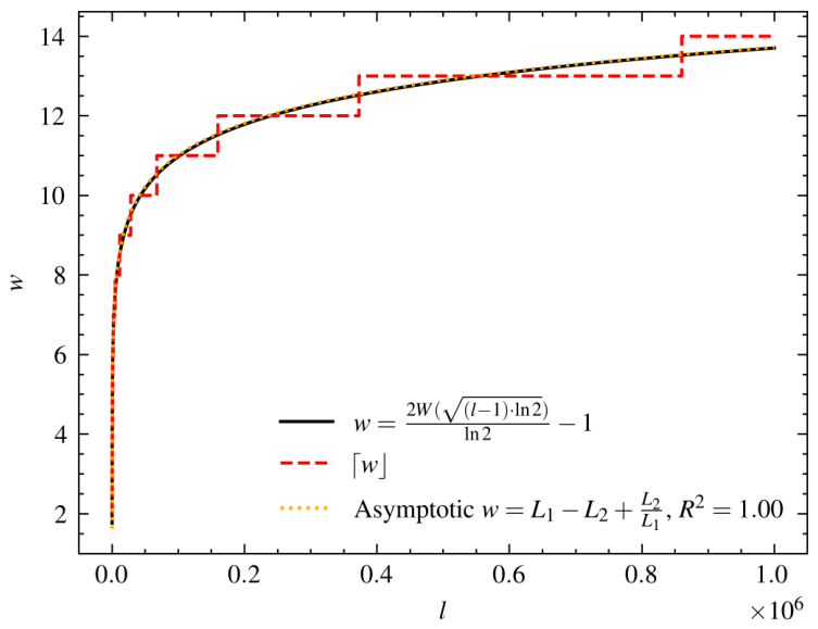
Let $f\left(w\right)=2^{w-1}-1+{\displaystyle \frac{l-1}{w+1}}$ ($w\in \mathbb{Z}$ and $1\le w\le l$), then $f^{\prime }\left(w\right)=ln2·2^{w-1}-{\displaystyle \frac{l-1}{{(w+1)}^2}}$. Solve the inequality $f^{\prime }\left(w\right)\ge 0$, it infers that $w\ge {\displaystyle \frac{2\mathrm{AsymW}\left(\sqrt{(l-1)·ln2}\right)}{ln2}}-1$. We can draw the plot of $w\left(l\right)={\displaystyle \frac{2\mathrm{AsymW}\left(\sqrt{(l-1)·ln2}\right)}{ln2}}-1$ as Figure 2.

From Equation (4.19) in [11], it proves that while $\mathrm{AsymW}$ at infinity or at 0, it can be expressed as the following asymptotic formula

$$\mathrm{AsymW}\left(x\right)=L_1-L_2+{\displaystyle \frac{L_2}{L_1}}+O\left({\left({\displaystyle \frac{L_2}{L_1}}\right)}^2\right),$$

where $L_1=lnx$, $L_2=lnlnx$. In Figure 2, it shows that the fitting effect from asymptotic formula to exact result of $\mathrm{AsymW}$ is good, the coefficient of determination is close to 1.

Thus,

$$\begin{array}{cc}\hfill f{\left(w\left(l\right)\right)}_{min}& =f\left({\displaystyle \frac{2\mathrm{AsymW}\left(\sqrt{(l-1)·ln2}\right)}{ln2}}-1\right)\hfill \\ \hfill & \approx 2^{{\displaystyle \frac{2}{ln2}}\mathrm{AsymW}\left(\sqrt{(l-1)·ln2}\right)-2}-1+{\displaystyle \frac{l-1}{\mathrm{AsymW}\left(\sqrt{(l-1)·ln2}\right)}}\hfill \\ \hfill & \approx -7.9\times {10}^{-9}{l}^2+0.08l+1238.5,\hfill \end{array}$$

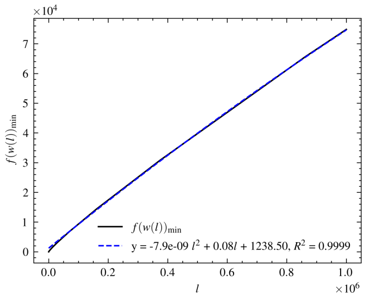
where $\mathrm{AsymW}\left(x\right)\approx L_1-L_2+{\displaystyle \frac{L_2}{L_1}}$, $L_1=lnx$ and $L_2=lnlnx$. Figure 3 shows that $f{\left(w\left(l\right)\right)}_{min}$ fits well with the approximation formula.    □

In Lemma 3, it infers that $T_{\mathrm{MP}}$ is nearly linear to the bit size of exponential number. Based on Lemma 3, we can derive the asymptotic complexity of the modular powering operation as $T_{\mathrm{MP}}(l,n)=\left(0.08l+1238.5\right)·T_{\mathrm{M}}\left(n\right)$.

2.2.3. Complexity of Normal Powering

A normal powering is always implemented by a simple binary algorithm (Section 4.6.3 algorithm A in [8]). Let e be an exponent and n be the bit size of base number, suppose $l=\lfloor {log}_{2}e\rfloor +1$ is the bit size of e. It costs around $\lfloor {log}_{2}e\rfloor +v\left(e\right)\le 2\lfloor {log}_{2}e\rfloor +1=2l-1$ multiplications in a normal powering computation, where $v\left(e\right)$ is the amount of 1’s in binary type of e. Let $T_{\mathrm{NP}}=(2l-1)·T_{\mathrm{M}}\left(n\right)$.

2.2.4. Complexity of the Greatest Common Divisor

Let n be the larger size in two integers. It usually uses an $O\left(n^2\right)$ binary style GCD algorithm (Section 4.5.2 algorithm B in [8]). So, we will regard $O\left(n^2\right)$ as the complexity of GCD algorithm. Let $T_{\mathrm{GCD}}\left(n\right)=O\left(n^2\right)=C_2·n^2+o\left(n^2\right)$.

2.3. Normal Multiplication Technique

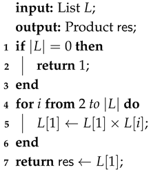
Beyond these fundamental operations, some variants of Pollard’s P-1 algorithm like IPP1 require computing the product of a massive list of primes. The Normal Multiplication (NM) (Algorithm 1) to obtain the product of the list L is as follows. Let $x_0=1$ be an initial state, it sequentially updates the accumulator by executing $x_0\leftarrow x_0·x$ for every $x\in L$.

As established in Corollary 1, multiplying all primes up to an n-bit integer via NM requires $T_{\mathrm{NMP}}\left(n\right)=\mathcal{O}\left(4^n\right)$ operations, yielding a massive product of bit-length ${\mathrm{bit}}_{\mathrm{LMP}}\left(n\right)$. To resolve this computational bottleneck, we adopt a divide-and-conquer Fast Multiplication (FM) strategy (Algorithm 7). FM reduces the time cost to $T_{\mathrm{FMP}}(n_1,n_2)=\mathcal{O}\left(2^{n_2}{(n_2-n_1)}^2\right)$ operations (see Corollary 2).

2.4. Overview of Pollard’s P-1 Algorithm and Its Development

Without loss of generality, we assume that the largest prime factor of $P-1$ is less than or equal to that of $Q-1$. Let a be a randomly chosen positive integer satisfying $gcd(a,N)=1$. By Fermat’s Little Theorem, any exponent z that is a multiple of $P-1$ satisfies ${\left[a^z\right]}_P\equiv 1$. This implies that P divides $a^z-1$, allowing us to efficiently extract the prime factor P by evaluating $gcd({[a^z-1]}_N,N)$. Based on this fundamental property, Pollard proposed the $P-1$ algorithm [3], which strategically constructs the exponent z using the prime set $\mathcal{P}$. Specifically, by setting $z={\prod }_{p_i\in \mathcal{P}}{p}_i^{e_i}$ with sufficiently large algorithmic exponents $e_i$, the algorithm guarantees that $(P-1)\mid z$, thereby successfully factorizing N. Depending on the specific strategies used to construct this exponent z, several variants have emerged. In the remainder of this section, we review the original algorithm alongside its two prominent variants [5,6].

Algorithm 1: Normal Multiplication Method

2.4.1. Original Pollard’s P-1 Algorithm [3]

To translate the aforementioned theory into practice, Pollard’s original work [3] proposed a practical two-stage approach. Let $B_1$ and $B_2$ be positive integers such that $1<B_1<B_2<B_1^2\le N^{1/2}$. If N is divisible by a prime factor P, the algorithm succeeds under two conditions: Stage 1. $P-1$ is a $B_1$-smooth number; or Stage 2. $P-1=Ap$, where A is a $B_1$-smooth number and $B_1<p<B_2$ is a prime.

In practice, executing Stage 1 requires constructing an exponent z that covers all prime powers up to the bound $B_1$. While the original paper establishes this framework, it does not explicitly specify the valuation rule for the corresponding algorithmic exponents $e_i$. To address this and ensure that $p_i^{e_i}\le B_1$, subsequent formulations like Rabah’s [12] formally define $e_i$ as $e_i=\lfloor {\displaystyle \frac{log{B}_1}{log{p}_i}}\rfloor$.

2.4.2. Pollard’s P-1 Algorithm in [5]

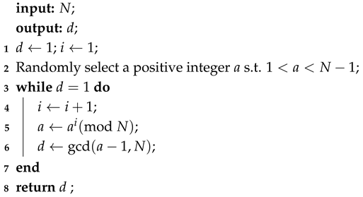
To bypass the need for a predetermined smoothness bound, a trivial variant (Algorithm 2) proposed by Bishop [5] simply increments an integer multiplier step-by-step. Starting with a random base $a\in (1,N-1)$, the method iterates through $i=2,3,4,\dots$, sequentially updating $a\leftarrow {\left[a^i\right]}_N$ and checking $d=gcd(a-1,N)$ at each step until a non-trivial factor is found. While this exhaustive linear enumeration theoretically guarantees eventual factorization, its increment-by-one nature results in an impractically large computational overhead.

Algorithm 2: Trivial Pollard’s P-1 Algorithm in [5]

2.4.3. Pollard’s P-1 Algorithm in [6]

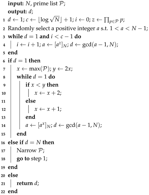
In 2022, Somsuk [6] proposed an improved variant of Pollard’s P-1 algorithm, denoted as $\mathsf{I}\mathsf{P}\mathsf{P}\mathsf{1}$ (Algorithm 3). Instead of processing primes individually, $\mathsf{I}\mathsf{P}\mathsf{P}\mathsf{1}$ first computes the product of all prime numbers within a predefined list $\mathcal{P}$ (i.e., $z={\prod }_{p\in \mathcal{P}}p$). It then repeatedly performs the modular exponentiation $a\leftarrow {\left[a^z\right]}_N$ and evaluates the GCD, iterating up to a maximum bound (e.g., $\lfloor log\sqrt{N}\rfloor +1$). As established in Section 2.2.2, the cost of a single modular exponentiation is roughly $0.08l+1238.50$ operations (where l is the exponent’s bit size). Consequently, aggregating primes into a single product z before exponentiation is computationally cheaper than performing consecutive modular exponentiations for each eligible prime. This strategy effectively reduces the running cost when the exponents of $(P-1)$’s prime factors are relatively uniform. However, because $\mathsf{I}\mathsf{P}\mathsf{P}\mathsf{1}$ uniformly raises all primes in $\mathcal{P}$ to the same iterative power, the overall cost increases drastically if even one prime factor possesses a large exponent, as it forces redundant exponentiations for the rest of the primes (Note that [6] also proposed a second version ($\mathsf{I}\mathsf{P}\mathsf{P}\mathsf{1}\text{\_}\mathsf{V}\mathsf{2}$) incorporating a linear step-by-step search as a fallback when the initial bound fails. However, since this fallback mechanism essentially mirrors the impractically expensive trivial variant discussed earlier, our analysis fundamentally focuses on $\mathsf{I}\mathsf{P}\mathsf{P}\mathsf{1}$’s core aggregated-exponentiation strategy.).

Algorithm 3: $\mathsf{I}\mathsf{P}\mathsf{P}\mathsf{1}$: Improved Pollard’s P-1 Algorithm in [6]

3. Dynamic Scaling Pollard’s P-1 Algorithm and Its Analysis

In this section, we present the details of our proposed Dynamic Scaling Pollard’s P-1 ($\mathsf{DSP}$) algorithm (Section 3.1). As previously discussed, existing methods either suffer from static bound-guessing (traditional $P-1$) or incur massive redundant exponentiations when prime factors require uneven powers ($\mathsf{I}\mathsf{P}\mathsf{P}\mathsf{1}$). To overcome these limitations, $\mathsf{DSP}$ introduces a dynamic scaling strategy that synergistically advances both the prime candidates and their respective exponents. By restructuring the traversal order and continuously reusing intermediate prime products, our variant efficiently bounds the exponents up to $n_N/2-1$ bits while incorporating timely GCD evaluations. Then, we provide an example to explain our improvement over $\mathsf{I}\mathsf{P}\mathsf{P}\mathsf{1}$ in Section 3.2. Finally, we give two complexity estimators for $\mathsf{DSP}$ and $\mathsf{I}\mathsf{P}\mathsf{P}\mathsf{1}$ and a detailed theoretical analysis about their costs in Section 3.3.

3.1. Main Algorithm

As detailed in Algorithm 4, $\mathsf{DSP}$ takes two primary inputs: the RSA modulus N and a smoothness bound $\gamma$. The parameter $\gamma$ serves as the global upper bound for the prime candidate list $\mathcal{P}$ with size t. By default, it can be set to the theoretical maximum $\gamma =2^{n_N/2-1}$ to guarantee the extraction of P in the worst-case scenario. However, it strategically allows users to supply a tighter bound to significantly accelerate the factoring process if partial prior knowledge regarding the smoothness of $P-1$ is available.

Upon receiving these inputs, the algorithm begins its initialization. Since $P-1$ is inherently even, we first eliminate its factor of 2 by pre-squaring the initial base $a=2$, computing $b\leftarrow {\left[a^2\right]}_N$, and checking $gcd(b-1,N)$ (lines 1–3). If N remains unfactored after this initial check, $\mathsf{DSP}$ proceeds to its core dynamic scaling phase to compute $b\leftarrow {\left[2^{{\prod }_{p_i\in \mathcal{P}}{p}_i^{e_i}}\right]}_N$. To minimize redundant modular exponentiations and maximize overall computational efficiency, this computation processes the primes iteratively in carefully bounded subsets.

Algorithm 4: Dynamic Scaling Pollard’s P-1 Algorithm

Let $P_j$, $P_{j,1}$, and $P_{j,2}$ denote the exponent applied in the j-th iteration and its intermediate constructive components, respectively. As initialized in line 5, we set $P_{0,2}=2$ and $P_{1,1}=P_{0,2}$. The algorithm then iterates j from 1 to $k_0$. For iterations where $j<k_0$, we generate the j-th prime subset ${\mathcal{P}}_j$ bounded by $2^{2^j}$ and compute its product $P_{j,2}=max\{1,{\prod }_{p\in {\mathcal{P}}_j}p\}$. The dynamic exponent is then constructed as $P_j=P_{j,1}·P_{j,2}$, and the accumulator for the next iteration is updated as $P_{(j+1),1}=P_{j,1}·P_j$. In the final iteration of this phase (i.e., $j=k_0$), we simply assign $P_{k_0}=P_{k_0,1}$ (lines 14–15). After determining $P_j$ in each iteration, we exponentiate it to the base b via $b\leftarrow {\left[b^{P_j}\right]}_N$ (line 16). Following each exponentiation, we test whether $d=gcd(b-1,N)$ yields a non-trivial factor. If $d\ne 1$, we have successfully recovered the prime $P=d$; otherwise, the iteration continues.

The objective of these steps is to ensure that all possible prime factors within ${\bigcup }_{j=1}^{k_0-1}{\mathcal{P}}_j$ are exponentiated to the base b with sufficiently high exponents after $k_0$ iterations. Based on the constructive steps, we can explicitly unroll the recurrence relations as $P_j=P_{j,2}·{\prod }_{i=0}^{j-1}{P}_{i,2}^{2^{j-i-1}}$ and $P_{(j+1),1}={\prod }_{i=0}^j{P}_{i,2}^{2^{j-i}}$. Consequently, after the $k_0$-th iteration completes, the base b inherently accumulates to $b\equiv {[2^{{\prod }_{j=0}^{k_0-1}{P}_{j,2}^{2^{k_0-j}}}]}_N={[2^{{\prod }_{p_i\in {\bigcup }_{j=1}^{k_0-1}{\mathcal{P}}_j}{p}_i^{e_i}}]}_N$. This guarantees that the accumulated exponent perfectly covers the required upper bounds $e_i$ for all primes in the generated subsets. If all prime factors of $P_{\mathrm{div}}$ reside in ${\bigcup }_{j=1}^{k_0-1}{\mathcal{P}}_j$, the algorithm ensures that P will be extracted.

If N remains unfactored after the loop, Phase 2 (lines 21–30) is triggered. We do not need to multiply and fully exponentiate all primes in the final subset ${\mathcal{P}}_{k_0}$. Since any prime in this set is strictly greater than $2^{2^{k_0-1}}$, assuming two such primes divide $P_{\mathrm{div}}$ yields a mathematical contradiction: $p_1{p}_2>2^{2^{k_0}}>P_{\mathrm{div}}$. Thus, $P_{\mathrm{div}}$ has at most one prime factor in ${\mathcal{P}}_{k_0}$. We bypass full modular exponentiations and instead apply Pollard’s shift modular exponentiation [3], efficiently computing $b\leftarrow {[b·a^{p-p_0}]}_N$ where $p-p_0$ is the gap between consecutive prime candidates.

Furthermore, during the implementation of our variant, we observed that directly computing the prime subset products $P_{j,2}$ poses a significant computational bottleneck. To address this, we optimized the naive multiplication method by adopting a fast multiplication algorithm, which significantly accelerates the processing of the prime lists. Detailed descriptions and complexity analyses of this improvement are provided in Section 4.

3.2. Comparison of Our Algorithm with $\mathsf{I}\mathsf{P}\mathsf{P}\mathsf{1}$

$\mathsf{I}\mathsf{P}\mathsf{P}\mathsf{1}$ tries to increase the utilization of the product of certain prime factors, but it can only increase efficiency when all the exponents of the prime factors are small. The probability of a small $u_{\max }$ occurring is very low; therefore, we aim to minimize the cost of computing the product of numerous prime factors of $P_{\mathrm{div}}$ (below some upper bound) and increase the utilization of the product of certain prime factors. Our variant dynamically scales each $p_i^{u_i}$ from the bit size of $p_i$ to the bit size $n_N/2-1$, reuses the product of prime factors during exponentiation, and employs a dynamic strategy to maximize the usage rate. We provide Example 1 to illustrate why the product can be reused in the exponentiation operation and how it reduces the computation cost:

Example 1.

Given two different random prime numbers $p_1$ and $p_2$, and a base integer a coprime to a large integer N, there are two methods to compute ${[a^{{\left(p_1{p}_2\right)}^2}]}_N$:

(1) First, compute the product $X_1=p_1{p}_2$, and then iteratively compute exponentiation by $X_1$ twice, i.e., calculate $A={\left[a^{X_1}\right]}_N$ followed by ${[a^{X_1^2}]}_N\equiv {\left[A^{X_1}\right]}_N$.

(2) Directly compute the exponent $X={\left(p_1{p}_2\right)}^2$ and then calculate ${\left[a^X\right]}_N$.

Let $T_{1,1}$ be the cost of computing $X_1$ in case (1), and $T_{1,2}$ be the cost of computing the modulo exponentiation twice in case (1). Let $T_{2,1}$ be the cost of computing X in case (2), and $T_{2,2}$ be the cost of computing ${\left[a^X\right]}_N$ in case (2). Let $T_1=T_{1,1}+T_{1,2}$ be the total cost of case (1), and $T_2=T_{2,1}+T_{2,2}$ be the total cost of case (2).

Since Lemma 3 proves that the cost of modulo exponentiation $T_{\mathrm{MP}}$ is nearly linear to the bit size of the exponent, and given that the bit size of X is approximately twice that of $X_1$ (i.e., $\mathrm{bit}\left(X\right)\approx 2\mathrm{bit}\left(X_1\right)$), it implies that $T_{1,2}\approx T_{2,2}$.

However, it is obvious that computing the product $X={\left(p_1{p}_2\right)}^2$ incurs a higher cost than computing $X_1=p_1{p}_2$ (the former requires one additional squaring operation). Thus, $T_{2,1}>T_{1,1}$, which infers that $T_1<T_2$.

In $\mathsf{DSP}$, we apply this principle to save the computational cost of evaluating ${[a^{{\prod }_{i=1}^t{p}_i^{e_i}}]}_N$ by utilizing a dynamic strategy that reuses earlier products.

3.3. Cost Analysis of $\mathsf{I}\mathsf{P}\mathsf{P}\mathsf{1}$ and $\mathsf{DSP}$

The complexity analysis of the following algorithms only considers the solvable situation, excluding the failure scenario. To establish a unified evaluation framework for both $\mathsf{I}\mathsf{P}\mathsf{P}\mathsf{1}$ and our $\mathsf{DSP}$ variant, we decompose their execution loops into four fundamental operational costs. Regardless of the specific scaling strategy, the step-wise cost (see Section 2.2 and Corollary 2) in any given phase comprises: (1) computing the product of prime candidates within a designated interval (typically via Fast Multiplication, denoted as $T_{\mathrm{FMP}}$), (2) updating the applied exponent via standard integer multiplication ($T_{\mathrm{M}}$), (3) performing the core modular exponentiation ($T_{\mathrm{MP}}$), and (4) evaluating the greatest common divisor ($T_{\mathrm{GCD}}$).

3.3.1. Complexity Analysis of $\mathsf{I}\mathsf{P}\mathsf{P}\mathsf{1}$

We first propose a cost estimator for Algorithm 3 to accurately simulate the cost of Algorithm 3 as Algorithm 5 and then give a theorem about the complexity of Algorithm 3 as Theorem 1.

Algorithm 5: $\mathsf{I}\mathsf{P}\mathsf{P}\mathsf{1}$Est

input: $n_N$, $p_t$, $u_{\max }$; output: $T_{\mathsf{I}\mathsf{P}\mathsf{P}\mathsf{1}}$; 1  $n_{p_t}\leftarrow \lfloor log{p}_t\rfloor +1$; $n_{P_{1,1}}\leftarrow 1$; 2  $T_{\mathrm{FMP}},n_{\mathrm{FMP}}\leftarrow \mathtt{FastMulCostEst}(1,n_{p_t},Pr\left(n\right)={\displaystyle \frac{1}{nln2}})$; 3  $T\leftarrow T_{\mathrm{FMP}}+u_{\max }{T}_{\mathrm{MP}}(n_{\mathrm{FMP}},n_N)+u_{\max }{T}_{\mathrm{GCD}}\left(n_N\right)$; 4  return T;

Theorem 1.

(Cost Estimation for [6]) If $p_t\ge p_{{\sigma }_s}$, then N can be factored by Algorithm 3 at most

$$\begin{array}{cc}\hfill T_{\mathsf{I}\mathsf{P}\mathsf{P}\mathsf{1}}(p_t,u_{\max },n_N)=& C_1{p}_t{log}^2{p}_t+u_{\max }{C}_2{n}_N^2\hfill \\ \hfill & +u_{\max }{C}_1{p}_t{n}_{N}log\left(n_N\right)+o(u_{\max }{p}_t{n}_{N}log\left(n_N\right)).\hfill \end{array}$$

(2)

Especially, if $p_t=p_{{\sigma }_s}$, the cost is

$$\begin{array}{cc}\hfill T_{\mathsf{I}\mathsf{P}\mathsf{P}\mathsf{1}}(p_{{\sigma }_s},u_{\max },n_N)=& C_1{p}_{{\sigma }_s}{log}^2{p}_{{\sigma }_s}+u_{\max }{C}_2{n}_N^2\hfill \\ \hfill & +u_{\max }{C}_1{p}_{{\sigma }_s}{n}_{N}log\left(n_N\right)+o(u_{\max }{p}_{{\sigma }_s}{n}_{N}log\left(n_N\right)).\hfill \end{array}$$

(3)

Proof. 

The cost for implementing Algorithm 3 while $p_t\ge p_{{\sigma }_s}$ can be divided into three parts, product cost of $z={\prod }_{p_i\in B}{p}_i$, iterative modular powering for $a={\left[a^z\right]}_N$ and iterative GCD algorithm after each modular powering. According to Corollary 2, it takes no more than $T_{\mathrm{FMP}}\left(n_t\right)$ operations to compute the product cost of $z={\prod }_{p_i\in B}{p}_i$ and will get the z with bit size $n_z\left(p_t\right)={\mathrm{bit}}_{\mathrm{LMP}}\left(n_t\right)={\displaystyle \frac{2^{n_t}(n_t-1)+1}{n_{t}ln2}}$, where $n_t=\lceil log{p}_t\rceil$.

It takes around $T_{\mathrm{MP}}\left(n_z\left(p_t\right)\right)·T_{\mathrm{M}}\left(n_N\right)$ operations to compute the modular powering result with base a, exponent P and modulo N. It costs $T_{\mathrm{GCD}}\left(n_N\right)$ to compute a GCD. From Lemma 3, $\mathrm{AsymW}(\sqrt{(n_z\left(p_t\right)-1)·ln2})\approx {\displaystyle \frac{n_t}{2}}ln2+ln\left({\displaystyle \frac{n_t}{2}}ln2\right)+{\displaystyle \frac{ln\left(\frac{n_t}{2}ln2\right)}{\frac{n_t}{2}ln2}}$ and $T_{\mathrm{MP}}(n_z\left(p_t\right),n_N)\approx 2^{n_t}{T}_{\mathrm{M}}\left(n_N\right)$.

In the declaration of Algorithm 3, the maximal exponent of prime factor in $P-1$ is $\left(\lfloor logN\rfloor +1\right)$, we will solve N after $u_{\max }$ iterations of modular powering and GCD step. Thus, the total cost is

$$\begin{array}{cc}\hfill T_{\mathsf{I}\mathsf{P}\mathsf{P}\mathsf{1}}(p_t,u_{\max },n_N)=& T_{\mathrm{FMP}}\left(n_t\right)+u_{\max }·T_{\mathrm{GCD}}\left(n_N\right)+u_{\max }·T_{\mathrm{MP}}\left(n_z\left(p_t\right)\right)\hfill \\ \hfill =& C_1{2}^{n_t}{n}_t^2+u_{\max }{C}_2{n}_N^2+u_{\max }·C_1·2^{n_t}{n}_{N}log\left(n_N\right)\hfill \\ \hfill & +o(u_{\max }·2^{n_t}{n}_{N}log\left(n_N\right)),\hfill \\ \hfill =& C_1{p}_t{log}^2{p}_t+u_{\max }{C}_2{n}_N^2+u_{\max }·C_1·p_t{n}_{N}log\left(n_N\right)\hfill \\ \hfill & +o(u_{\max }·p_t{n}_{N}log\left(n_N\right)).\hfill \end{array}$$

   □

3.3.2. Complexity Analysis of Dynamic Scaling Pollard’s P-1 Algorithm

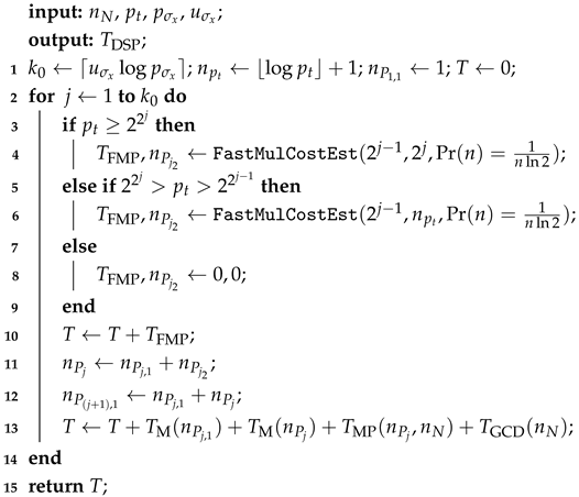
We first propose a cost estimator for Dynamic Scaling Pollard’s P-1 Algorithm to accurately simulate the cost of our variant as Algorithm 6 and then give a theorem about the complexity of our variant as Theorem 2.

Algorithm 6: $\mathsf{DSP}$Est

Theorem 2.

(Cost Estimation for Our Variant) The complexity in factoring N successfully by our Dynamic Scaling Pollard’s P-1 Algorithm (Algorithm 4) is as follows,

If $p_{{\sigma }_s}\le 2^{2^{k_0-1}}$, then the cost of Dynamic Scaling Pollard’s P-1 Algorithm is

$$\begin{array}{ccc}\hfill T_{\mathrm{DSP}}(p_{{\sigma }_s},p_{{\sigma }_x},u_{{\sigma }_x},n_N)& =& log(u_{{\sigma }_x}log{p}_{{\sigma }_x})C_2{n}_N^2\hfill \\ \hfill & & +C_1{p}_{{\sigma }_s}({\displaystyle \frac{1}{4}}{log}^2{p}_{{\sigma }_s}-log{p}_{{\sigma }_s}+u_{{\sigma }_x}log{p}_{{\sigma }_x}+1)\hfill \\ \hfill & & +C_1{p}_{{\sigma }_s}{\displaystyle \frac{2u_{{\sigma }_x}log{p}_{{\sigma }_x}}{log{p}_{{\sigma }_s}}}{n}_{N}log{n}_N+o(u_{{\sigma }_x}{p}_{{\sigma }_s}log{p}_{{\sigma }_x}).\hfill \end{array}$$

(4)

Proof. 

(1) If $p_{{\sigma }_s}\le 2^{2^{k_0-1}}$, N will be factored in the process of Algorithm 4 declared from line 9 to 31 with $k_0=log\left(u_{{\sigma }_x}log{p}_{{\sigma }_x}\right)$ loops. The cost in case (1) contains the computations of set $P_{j,2}$, $P_j$ and $P_{(j+1),1}$, the modular powering operation $b={\left[b^{P_j}\right]}_N$ for each element $P_j$ from $j=1$ to k and a GCD operation in the end of each iteration.

For set $B_j$, the minimal bit size of $p\in B_j$ is $2^{j-1}+1$ and the maximal bit size of $p\in B_j$ is $2^j$. Let $k_1=loglog{p}_{{\sigma }_s}\le k_0$, according to Corollary 2 and the description of line 12 in Algorithm 4, it takes no more than

$$\left\{\begin{array}{cc}{T}_{\mathrm{FMP}}(2^{j-1},2^j),& 2\le j\le k_1,\\ 0,& k_0\ge j>k_1,\end{array}\right.$$

to compute the product cost of $P_{j,2}={\prod }_{p\in B_j}p$ and will get $P_{j,2}$ with the bit size

$$\mathrm{bit}\left(P_{j,2}\right)=\left\{\begin{array}{cc}{\mathrm{bit}}_{\mathrm{LM}}(2^{j-1},2^j),& 2\le j\le k_1,\\ 0,& k_0\ge j>k_1.\end{array}\right.$$

Since $P_{j,1}={\prod }_{i=0}^{j-1}{P}_{i,2}^{2^{j-i-1}}$, $n_{P_{0,2}}=1$ and $n_{P_{12}}={\mathrm{bit}}_{\mathrm{LM}}\left(2\right)-n_{P_{0,2}}$, it infers that the bit size of $P_{j,1}$ is

$$\begin{array}{cc}\hfill \mathrm{bit}\left(P_{j,1}\right)& ={\displaystyle \sum _{i=0}^{j-1}}{2}^{j-i-1}\mathrm{bit}\left(P_{i,2}\right)\hfill \\ \hfill & =2^{j-1}+{\displaystyle \sum _{i=1}^{j-1}}{2}^{j-i-2}{\mathrm{bit}}_{\mathrm{LM}}(2^{i-1},2^i)<{\displaystyle \frac{2^{2^{j-1}}+3·2^{2^{j-2}}}{2ln2}}\hfill \end{array}$$

while $2\le j\le k_1+1$ and

$$\mathrm{bit}\left(P_{j,1}\right)=2\mathrm{bit}\left(P_{(j-1),1}\right)=2^{j-(k_1+1)}\mathrm{bit}\left(P_{(k_1+1),1}\right)$$

for $k_0\ge j>k_1+1$.

The cost for computing each $P_j$ is $T_{\mathrm{M}}\left(\mathrm{bit}\left(P_{j,1}\right)\right)$ and get $P_j$ with the bit size

$$\mathrm{bit}\left(P_j\right)=\mathrm{bit}\left(P_{j,1}\right)+\mathrm{bit}\left(P_{j,2}\right)<\left\{\begin{array}{cc}{\displaystyle \frac{2^{2^j}}{ln2}},& 2\le j\le k_1,\\ {\displaystyle \frac{2^{2^{k_1}+j-(k_1+1)}}{ln2}},& k_0\ge j>k_1.\end{array}\right.$$

The cost for computing each $P_{(j+1),1}$ is $T_{\mathrm{M}}\left(\mathrm{bit}\left(P_j\right)\right)$.

The cost for modular powering operation $b\leftarrow {\left[b^{P_j}\right]}_N$ is $T_{\mathrm{MP}}\left(\mathrm{bit}\left(P_j\right)\right)·T_{\mathrm{M}}\left(n_N\right)$ and the GCD operation costs $T_{\mathrm{GCD}}\left(n_N\right)$ in each loop. From Lemma 3, we can get that

$$\begin{array}{cc}\hfill & \mathrm{AsymW}(\sqrt{(n_{P_j}-1)·ln2})\hfill \\ \hfill \approx & \left\{\begin{array}{cc}{2}^{j-1}ln2-ln(2^{j-1}ln2),& 2\le j\le k_1,\hfill \\ (2^{k_1}+{\displaystyle \frac{j-k_1-1}{2}})ln2-ln[(2^{k_1}+{\displaystyle \frac{j-k_1-1}{2}})ln2],& k_0\ge j>k_1,\hfill \end{array}\right.\hfill \end{array}$$

and

$$\begin{array}{c}\hfill T_{\mathrm{MP}}(\mathrm{bit}\left(P_j\right),n_N)<\left\{\begin{array}{cc}{2}^{2^j-2}·T_{\mathrm{M}}\left(n_N\right),& 2\le j\le k_1,\hfill \\ 2^{2^{k_1}+j-k_1-2}·T_{\mathrm{M}}\left(n_N\right),& k_0\ge j>k_1.\hfill \end{array}\right.\end{array}$$

So the total cost is

$$\begin{array}{cc}\hfill & T_{\mathrm{DSP}}(p_{{\sigma }_x},u_{{\sigma }_x},n_N)\hfill \\ \hfill =& {\displaystyle \sum _{j=1}^{k_1}}{T}_{\mathrm{FMP}}(2^{j-1}+1,2^j)+{\displaystyle \sum _{j=1}^{k_0}}\left[T_{\mathrm{M}}\left(\mathrm{bit}\left(P_{j,1}\right)\right)+T_{\mathrm{M}}\left(\mathrm{bit}\left(P_j\right)\right)+T_{\mathrm{MP}}(\mathrm{bit}\left(P_j\right),n_N)+T_{\mathrm{GCD}}\left(n_N\right)\right]\hfill \\ \hfill =& k_0{C}_2{n}_N^2+2C_1{2}^{2^{k_1}}{(2^{k_1-1}-1)}^2+C_1\left[2^{2^{k_1}-2}+2^{2^{k_1}+k_0-k_1-1}\right]n_{N}log{n}_N\hfill \\ \hfill & +C_1{2}^{k_0-k_1-1}{\displaystyle \frac{2^{2^{k_1}}+3·2^{2^{k_1-1}}}{2ln2}}log\left({\displaystyle \frac{2^{2^{k_1}}+3·2^{2^{k_1-1}}}{2ln2}}\right)+o(2^{2^{k_1}+k_0})\hfill \\ \hfill & +{\displaystyle \frac{1}{ln2}}\left[2^{2^{k_1}+1}log(2^{2^{k_1}+1})+2^{2^{k_1}+k_0-k_1-1}log\left(2^{2^{k_1}+k_0-k_1-1}\right)\right]\hfill \\ \hfill =& k_0{C}_2{n}_N^2+2C_1{2}^{2^{k_1}}{(2^{k_1-1}-1)}^2+C_1{2}^{2^{k_1}+k_0-k_1}{n}_{N}log{n}_N+O(2^{2^{k_1}+k_0})\hfill \\ \hfill =& log(u_{{\sigma }_x}log{p}_{{\sigma }_x})C_2{n}_N^2+C_1{p}_{{\sigma }_s}{({\displaystyle \frac{log{p}_{{\sigma }_s}}{2}}-1)}^2+C_1{p}_{{\sigma }_s}{\displaystyle \frac{2u_{{\sigma }_x}log{p}_{{\sigma }_x}}{log{p}_{{\sigma }_s}}}{n}_{N}log{n}_N\hfill \\ \hfill & +O(u_{{\sigma }_x}{p}_{{\sigma }_s}log{p}_{{\sigma }_x})\hfill \\ \hfill =& log(u_{{\sigma }_x}log{p}_{{\sigma }_x})C_2{n}_N^2+C_1{p}_{{\sigma }_s}\left({\displaystyle \frac{1}{4}}{log}^2{p}_{{\sigma }_s}-log{p}_{{\sigma }_s}+1+O(u_{{\sigma }_x}log{p}_{{\sigma }_x})\right)\hfill \\ \hfill & +C_1{p}_{{\sigma }_s}{\displaystyle \frac{2u_{{\sigma }_x}log{p}_{{\sigma }_x}}{log{p}_{{\sigma }_s}}}{n}_{N}log{n}_N+o(u_{{\sigma }_x}{p}_{{\sigma }_s}log{p}_{{\sigma }_x}).\hfill \end{array}$$

   □

4. Fast Multiplication Technique and Its Analysis

This section details our Fast Multiplication (FM) method (Section 4.1). We provide formal cost estimators and theoretical complexity analyses for both NM (see Section 2.2) and FM methods in Section 4.2, followed by experimental validation in Section 4.3. Ultimately, we demonstrate theoretically and empirically that standard multiplication incurs a time overhead ${\displaystyle \frac{2^{n+1}}{n^2}}$ times higher than FM when computing the product of all primes up to n bits.

4.1. Fast Multiplication Technique

Given a list $L=(x_1,\cdots ,x_k)$ defined in Section 2, NM introduced in Section 2.2 degrades rapidly for large lists because the accumulating product x grows drastically. Since computational cost depends heavily on the bit-length of the largest multiplier, this skewed growth inherently throttles efficiency. To accelerate it, we propose the FM algorithm (Algorithm 7). Given a sorted list L ($k>3$) of positive integers, FM operates recursively: During each iteration, if the current list length k is odd, a trivial multiplier 1 is prepended to the sequence. The elements are then extracted as $(x_1,\dots ,x_k)$ to pairwise multiply the symmetrically opposite ends: computing $x_i·x_{k-i+1}$ for $i=1,\dots ,k/2$. These temporary products form the updated sequence L, effectively halving the size parameter $k\leftarrow k/2$. This iterative process is repeated until only a single final product remains.

By continually balancing the bit-sizes of the intermediate multipliers, FM significantly reduces the calculation time compared to standard sequential multiplication. We mathematically formalize and prove this efficiency gain for uniformly distributed inputs in Section 4.3.

Algorithm 7: Fast Multiplication Method (FM)

4.2. Complexity Analysis of Normal Multiplication and Fast Multiplication

4.2.1. Complexity Analysis of Normal Multiplication Method

To fully evaluate the efficiency gains of our proposed algorithms, it is necessary to first analyze the time complexity of NM (Section 2.3). It computes the total product by iteratively multiplying elements one by one. Theorem 3 establishes the theoretical upper bound on the computational cost for computing the product of the list L.

Theorem 3

(Time Complexity of the NM). Assume $L(p,n)$ is an ascending list defined in Section 2 with a size strictly greater than 3. Multiplying all elements in L using the NM requires around $T_{\mathrm{NM}}(p,n)={\displaystyle \frac{7}{6}}{C}_1{p}^2{n}^2{4}^n+o\left(4^n{p}^2{n}^2\right)$ operations. In particular, when $p=1$, the computational cost is $T_{\mathrm{NM}}(1,n)={\displaystyle \frac{7}{6}}{C}_1{n}^2{4}^n+o\left(n^2{4}^n\right).$

Proof. 

Suppose the largest integer in list L is a and n is the bit size of a. Since p is the probability of a number $x\in [1,2^n-1]\cap \mathbb{Z}$ occurring in list L, the total amount of numbers in L is expected to be $p·(2^n-1)$. When $p=1$, the initial list L covers all positive integers up to $2^n-1$.

The normal multiplication method iteratively multiplies the elements in L. Let the accumulator be $L\left[1\right]$. For ease of discussion, we process the multipliers grouped by their bit sizes. In the iteration for bit size i (where $3\le i\le n$), we multiply the accumulator $L\left[1\right]$ by all elements in L that have exactly i bits (i.e., integers in the range $[2^{i-1},2^i-1]$). There are expected to be $p·2^{i-1}$ such multipliers.

According to Lemma 1, at the start of the iteration for bit size i, the expected bit size of the accumulator $L\left[1\right]$ is $b_{i-1}={\mathrm{bit}}_{\mathrm{LM}}(p,0,i-1)=p(i-2)2^{i-1}.$

During the iterations of bit size i, we perform $p·2^{i-1}$ multiplications. Each multiplier contributes approximately i bits to the accumulator. Therefore, the k-th multiplication in this stage involves an accumulator of bit size $b_{i-1}+i(k-1)$. Let $T_i$ be the computational cost for the iteration of bit size i. Considering the time cost of each multiplication $T_{\mathrm{M}}$ in Section 2.2.1, we have $T_i=C_1{\sum }_{k=1}^{p·2^{i-1}}(ik+b_{i-1})log(ik+b_{i-1})+o\left(i^2{4}^i\right)$. Since $log(i·p{2}^{i-1}+p{2}^{i-1}(i-2))=log\left(p{2}^i(i-1)\right)=i+log\left(p(i-1)\right)\approx i$ and $log(i+p{2}^{i-1}(i-2))\approx log\left(p{2}^{i-1}i\right)\approx i$ and Applying Lemma 2 by substituting $A=i$ and $B\approx b_{i-1}$, we have

$$\begin{array}{cc}\hfill T_i& =C_1{\displaystyle \sum _{k=1}^{p·2^{i-1}}}(ik+b_{i-1})log(ik+b_{i-1})+o\left(i^2{4}^i\right)\hfill \\ & \approx C_1\left[\left({\displaystyle \frac{1}{8}}{p}^{2}i{4}^i+{\displaystyle \frac{1}{4}}{p}^2{4}^i(i-2)+{\displaystyle \frac{1}{4}}{p}^2{4}^i{\displaystyle \frac{{(i-2)}^2}{i}}\right)·i+\left({\displaystyle \frac{1}{4}}{p}^2{4}^i{\displaystyle \frac{{(i-2)}^2}{i}}\right)·i\right]\hfill \\ & =C_1\left[p^2{4}^i\left({\displaystyle \frac{5}{8}}i-{\displaystyle \frac{3}{2}}+{\displaystyle \frac{1}{i}}\right)·i+{\displaystyle \frac{1}{4}}{p}^2{4}^i\left(i-4+{\displaystyle \frac{4}{i}}\right)·i\right]\hfill \\ & =C_1\left({\displaystyle \frac{5}{8}}{p}^2{i}^2{4}^i+{\displaystyle \frac{1}{4}}{p}^2{i}^2{4}^i\right)+o\left(i^2{4}^i\right)\hfill \\ & ={\displaystyle \frac{7}{8}}{C}_1{p}^2{i}^2{4}^i+o\left(i^2{4}^i\right).\hfill \end{array}$$

Thus, the total time complexity $T_{\mathrm{NM}}(p,n)$ is the summation of $T_i$ over all bit sizes i from 3 to n. Using the geometric series approximation ${\sum }_{i=1}^n{i}^2{4}^i\approx {\displaystyle \frac{4}{3}}{n}^2{4}^n$, we obtain:

$$\begin{array}{cc}\hfill T_{\mathrm{NM}}(p,n)& ={\displaystyle \sum _{i=3}^n}{T}_i+o\left(4^n{p}^2{n}^2\right)\hfill \\ & =C_1{\displaystyle \sum _{i=3}^n}\left({\displaystyle \frac{7}{8}}{p}^2{i}^2{4}^i-{\displaystyle \frac{5}{2}}{p}^{2}i{4}^i+2p^2{4}^i\right)+o\left(4^n{p}^2{n}^2\right)\hfill \\ & ={\displaystyle \frac{7}{6}}{C}_1{p}^2{n}^2{4}^n+o\left(4^n{p}^2{n}^2\right).\hfill \end{array}$$

In particular, when $p=1$, the computational cost simplifies to $T_{\mathrm{NM}}(1,n)={\displaystyle \frac{7}{6}}{C}_1{n}^2{4}^n+o\left(n^2{4}^n\right).$    □

Corollary 1.

For all prime numbers smaller or equal to the maximal n-bit positive integer $2^n-1$, it takes at most

$$\begin{array}{c}\hfill T_{\mathrm{NMP}}\left(n\right)=T_{\mathrm{NM}}({\displaystyle \frac{1}{nln2}},n)={\displaystyle \frac{7}{6{ln}^{2}2}}{C}_1{4}^n.\end{array}$$

(5)

operations to multiply all these numbers together by Algorithm 1 and get smaller than or equal to ${\mathrm{bit}}_{\mathrm{LMP}}\left(n\right)$-bit positive integer.

4.2.2. Complexity Analysis of FM

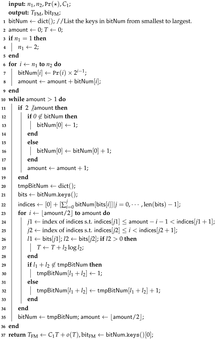
Due to the intricate nature of the complexity analysis for FM, we first propose a cost estimator to accurately simulate its computational overhead. Suppose L is a list containing strictly more than three distinct positive integers, where the minimum and maximum bit sizes of its elements are $n_1$ and $n_2$, respectively. Let p be the probability of an integer $x\in [1,2^{n_2}-1]\cap \mathbb{Z}$ appearing in L. The cost evaluation is formalized in Algorithm 8. By taking parameters $n_1$, $n_2$, and p as inputs, it returns the estimated computational cost $T_{\mathrm{FM}}(p,n_1,n_2)$.

Theorem 4.

(Cost of FM Algorithm) Assume $L(p,n_1,n_2)$ is an ascending list defined in Section 2 with a size strictly greater than 3. It takes roundly

$$T_{\mathrm{FM}}(p,n_1,n_2)=C_{1}p{2}^{n_2}{(n_2-n_1)}^2{n}_2+o\left(p{2}^{n_2}{(n_2-n_1)}^2{n}_2\right)$$

(6)

operations to compute the product of L by FM (Algorithm 7). Especially, while $p=1$, we have

$$T_{\mathrm{FM}}(1,n_1,n_2)=C_1{2}^{n_2}{(n_2-n_1)}^2{n}_2+o\left(2^{n_2}{(n_2-n_1)}^2{n}_2\right)$$

(7)

Algorithm 8: FastMulCostEst

Proof. 

Since the minimum and maximum bit size of integers in list L are $n_1$ and $n_2$ ($n_1<n_2$), the amount of the positive integers in the range of $[2^{n_1},2^{n_2}-1]$ is $2^{n_2}-2^{n_1}$ and p is the probability of a number $x\in \mathbb{Z}\cap [2^{n_1},2^{n_2}-1]$ occurring in list L. It infers that the initial list L could be $[2^{n_1},2^{n_1}+1,\cdots ,2^{n_2}-1]$ with size $2^{n_2}-2^{n_1}$ while $p=1$. We could add $2^{n_1}$ 1’s into L.

It performs $2^{n_2-1}-2^{n_1}$ non-trivial multiplications in the first fold-in-half stage. Since the amount of k-bit positive integers is $2^{k-1}$, it computes $2^{k-1}$ products of an $n_2$-bit number and a k-bit number for $n_1+1\le k\le n_2-1$ in each multiplication and remain $2^{n_1}$$n_2$-bit numbers. It costs $(2^{n_2-1}-2^{n_1})C_1{n}_{2}log{n}_2+(2^{n_2-1}-2^{n_1})·o(n_{2}log{n}_2)$ operations at the first-iter and obtains $2^{n_2-1}$ numbers in total and store them in an empty list L for next multiplications as

Table 1. Bit size in L after 1st iteration in FM.

Bit Size	$n_2$	$n_1+n_2+1$	$n_1+n_2+2$	⋯	$2n_2-1$	Total
Amount	$2^{n_1}$	$2^{n_1}$	$2^{n_1+1}$	⋯	$2^{n_2-2}$	$2^{n_2-1}$

.

For the second iteration, it performs $2^{n_2-2}$ multiplications. It computes $2^{n_1}$ products of a $(2n_2-1)$-bit number and an $n_2$-bit number in each multiplication, $2^{k-1}$ products of a $(2n_2-1)$-bit number and a $(n_2+k)$-bit number for $n_1+1\le k\le n_2-2$ in each multiplication. It costs $2^{n_2-2}{C}_1(2n_2-1)log(2n_2-1)+2^{n_2-2}o((2n_2-1)log(2n_2-1))$ operations at the second-iter and obtains $2^{n_2-2}$ numbers in total and store them in an empty list L for next multiplications as the

Table 2. Bit size in L after 2nd iteration in FM.

Bit Size	$3n_2-1$	$n_1+3n_2$	$n_1+3n_2+1$	⋯	$4n_2-3$	Total
Amount	$2^{n_1}$	$2^{n_1}$	$2^{n_1+1}$	⋯	$2^{n_2-3}$	$2^{n_2-2}$

.

For the i-th-iter ($i\le (n_2-n_1)$), it applies to $2^{n_2-i}$ multiplications. It computes $2^{n_1}$ products of a $(2^{i-1}{n}_2-2^{i-1}+1)$-bit number and a $[(2^{i-1}-1)n_2-2^{i-1}+i]$-bit number and $2^{k-1}$ products of a $(2^{i-1}{n}_2-2^{i-1}+1)$-bit number and a $[(2^{i-1}-1)n_2-2^{i-1}+i+k]$-bit number for $n_1+1\le k\le n_2-i$ in each multiplication. It costs $2^{n_2-i}{C}_1(2^{i-1}{n}_2-2^{i-1}+1)log(2^{i-1}{n}_2-2^{i-1}+1)+2^{n_2-i}·o((2^{i-1}{n}_2-2^{i-1}+1)log(2^{i-1}{n}_2-2^{i-1}+1))$ operations at the i-th-iter. It obtains $2^{n_2-i}$ numbers in total and store them in an empty list L for next multiplications as

Table 3. Bit size in L after i-th iteration in FM.

Bit Size	$\mathrm{b}\left(i\right)$ §	$n_1+\mathrm{b}\left(i\right)+1$	$n_1+\mathrm{b}\left(i\right)+2$	⋯	$2^i{n}_2-2^i+1$	Total
Amount	$2^{n_1}$	$2^{n_1}$	$2^{n_1+1}$	⋯	$2^{n_2-i-1}$	$2^{n_2-i}$

§ $\mathrm{b}\left(i\right)=(2^i-1)n_2-2^i+i+1$.

.

For the $(n_2-n_1)$-th-iter, it applies to $2^{n_1}$ multiplications. It computes $2^{n_1}$ products of a $(2^{n_2-n_1-1}(n_2-1)+1)$-bit number and a $(2^{n_2-n_1-1}(n_2-1)-n_1)$-bit number in each multiplication. It costs $2^{n_1}{C}_1(2^{n_2-n_1-1}(n_2-1)+1)log(2^{n_2-n_1-1}(n_2-1)+1)+2^{n_1}·o((2^{n_2-n_1-1}(n_2-1)+1)log(2^{n_2-n_1-1}(n_2-1)+1))$ operations at the $(n_2-n_1)$-th-iter, then we obtain $2^{n_1}$ products with bit size at most $\left(2^{n_2-n_1}(n_2-1)-n_1+1\right)$-bit.

For the $(n_2-n_1+i)$-th-iter ($1\le i\le n_1$), it applies to $2^{n_1-i}$ multiplications. It computes $2^{n_1-i}$ products of two $\left[2^{i-1}(2^{n_2-n_1}(n_2-1)-n_1+1)\right]$-bit numbers in each multiplication. It costs $2^{n_1-i}{C}_1\left[2^{i-1}(2^{n_2-n_1}(n_2-1)-n_1+1)\right]log\left[2^{i-1}(2^{n_2-n_1}(n_2-1)-n_1+1)\right]+2^{n_1-i}·o(\left[2^{i-1}(2^{n_2-n_1}(n_2-1)-n_1+1)\right]log\left[2^{i-1}(2^{n_2-n_1}(n_2-1)-n_1+1)\right])$ operations at the $(n_2-n_1+i)$-th-iter, then we obtain $2^{n_1-i}$ products with bit size at most $\left[2^i(2^{n_2-n_1}(n_2-1)-n_1+1)\right]$-bit. We get the last product of FM with bit size $[2^{n_2}(n_2-1)-2^{n_1}{n}_1+2^{n_1}]$ while $i=n_1$.

Let $b_1\left(i\right)=(2^{i-1}{n}_2-2^{i-1}+1)$, $b_2=2^{n_2-n_1+1}(n_2-1)-2n_1+2$, then

$$\begin{array}{cc}\hfill \mathrm{G}(1,n_1,n_2):=& (2^{n_2-1}-2^{n_1})n_{2}log{n}_2+{\displaystyle \sum _{i=2}^{n_2-n_1}}{2}^{n_2-i}{b}_1\left(i\right)log{b}_1\left(i\right)\hfill \\ \hfill & +{\displaystyle \sum _{i=1}^{n_1}}{2}^{n_1-i}{2}^{i-2}{b}_{2}log\left(2^{i-2}{b}_2\right)\hfill \\ \hfill =& (2^{n_2-1}-2^{n_1})n_{2}log{n}_2+{\displaystyle \sum _{i=2}^{n_2-n_1}}{2}^{n_2-i}{b}_1\left(i\right)log{b}_1\left(i\right)\hfill \\ \hfill & +n_1{2}^{n_1-2}{b}_{2}log{b}_2+2^{n_1-3}{b}_2{n}_1(n_1-3)\hfill \\ \hfill \le & (2^{n_2-1}-2^{n_1})n_{2}log{n}_2+{\displaystyle \sum _{i=2}^{n_2-n_1}}{2}^{n_2-i}{b}_1\left(i\right)log{b}_1(n_2-n_1+1)\hfill \\ \hfill & +n_1{2}^{n_1-2}{b}_{2}log{b}_2+2^{n_1-3}{b}_2{n}_1(n_1-3)\hfill \\ \hfill \le & [2^{n_2-1}{(n_2-n_1)}^2(n_2-1)+(2^{n_2-1}-2^{n_1})\left(2n_2-n_1\right)]log{n}_2\hfill \\ \hfill & +[2^{n_2-1}(n_2-1)-2^{n_1-1}{n}_1+2^{n_1}]n_1(n_2-n_1+1)log{n}_2\hfill \\ \hfill & +n_1(n_1-3)[2^{n_2-2}{n}_2-2^{n_2-2}-2^{n_1-2}{n}_1+2^{n_1-1}]\hfill \\ \hfill =& 2^{n_2}{(n_2-n_1)}^2{n}_2+o\left(2^{n_2}{(n_2-n_1)}^2{n}_2\right).\hfill \end{array}$$

All in all, we add up all the overhead and get the time cost of the FM (Algorithm 7):

$$\begin{array}{cc}\hfill T_{\mathrm{FM}}(1,n_1,n_2)& =C_1\mathrm{G}(1,n_1,n_2)+o\left(\mathrm{G}(1,n_1,n_2)\right)\hfill \\ \hfill & =C_1{2}^{n_2}{(n_2-n_1)}^2{n}_2+o\left(2^{n_2}{(n_2-n_1)}^2{n}_2\right).\hfill \end{array}$$

While $p<1$, it infers that the amount of numbers in list L is $p(2^{n_2}-2^{n_1})$. Thus, we get that the bit size of the product is ${\mathrm{bit}}_{\mathrm{LM}}(p,n_1,n_2)=p[2^{n_2}(n_2-1)-2^{n_1}(n_1-1)]$ and

$$\begin{array}{cc}\hfill \mathrm{G}(p,n_1,n_2):=& p\mathrm{G}(1,n_1,n_2)\hfill \\ \hfill =& p{2}^{n_2}{(n_2-n_1)}^2{n}_2+o\left(p{2}^{n_2}{(n_2-n_1)}^2{n}_2\right),\hfill \end{array}$$

the total cost is

$$\begin{array}{cc}\hfill T_{\mathrm{FM}}(p,n_1,n_2)=& p\mathrm{G}(1,n_1,n_2)\hfill \\ \hfill =& C_1\mathrm{G}(1,n_1,n_2)+o\left(\mathrm{G}(1,n_1,n_2)\right)\hfill \\ \hfill =& C_{1}p{2}^{n_2}{(n_2-n_1)}^2{n}_2+o\left(p{2}^{n_2}{(n_2-n_1)}^2{n}_2\right).\hfill \end{array}$$

□

Corollary 2.

For all prime numbers smaller or equal from $n_1$-bit to $n_2$-bit positive integer, it takes at most

$$T_{\mathrm{FMP}}(n_1,n_2)=C_1·2^{n_2}{(n_2-n_1)}^2+o\left(2^{n_2}{(n_2-n_1)}^2\right)$$

(8)

operations to multiply all these numbers together by Algorithm 7. Let $T_{\mathrm{FMP}}\left(n\right):=T_{\mathrm{FMP}}(0,n)$.

Proof. 

According to Prime Theorem, the number of primes in $\mathbb{Z}\cap [2^{n_1},2^{n_2}-1]$ is $k={\displaystyle \frac{2^{n_2}-1}{ln(2^{n_2}-1)}}-{\displaystyle \frac{2^{n_1-1}-1}{ln(2^{n_1-1}-1)}}\approx {\displaystyle \frac{(n_1-1)2^{n_2}-n_2{2}^{n_1-1}}{(n_1-1)n_{2}ln2}}$. We can regard the prime numbers declared in Corollary 2 as a non-repeated list L on $\mathbb{Z}\cap [2^{n_1},2^{n_2}-1]$, then the probability that each number occurs in L is $p={\displaystyle \frac{k}{2^{n_2}-2^{n_1-1}}}\approx {\displaystyle \frac{1}{n_{2}ln2}}$. According to Theorem 4, it takes at most

$$\begin{array}{cc}\hfill T_{\mathrm{FMP}}(n_1,n_2)=& T_{\mathrm{FM}}({\displaystyle \frac{1}{n_{2}ln2}},n_1,n_2)\hfill \\ \hfill =& C_1{\displaystyle \frac{1}{n_{2}ln2}}·2^{n_2}{(n_2-n_1)}^2{n}_2+o({\displaystyle \frac{1}{n_{2}ln2}}·2^{n_2}{(n_2-n_1)}^2{n}_2)\hfill \\ \hfill =& C_1·2^{n_2}{(n_2-n_1)}^2+o\left(2^{n_2}{(n_2-n_1)}^2\right)\hfill \end{array}$$

operations to multiply all these numbers together by Algorithm 7. □

4.3. Comparison Between Normal Multiplication Method and FM

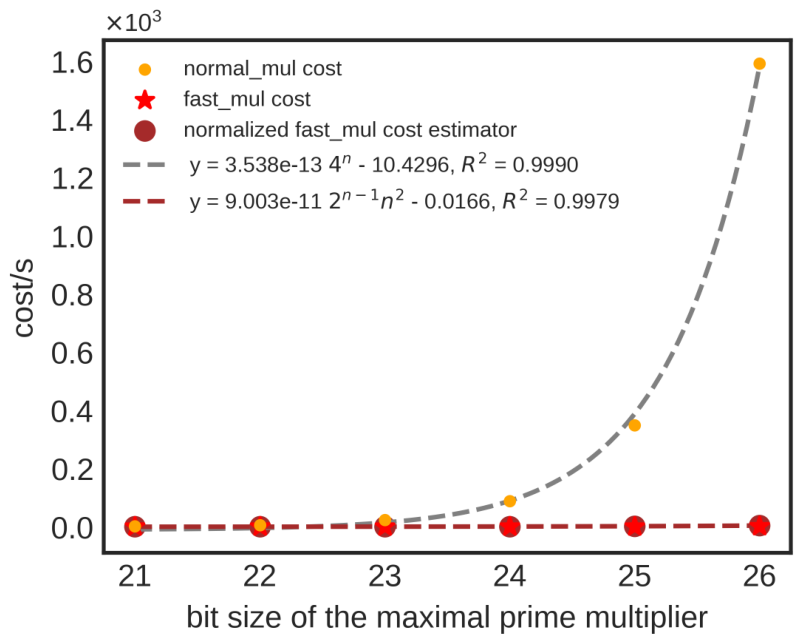
We give a comparison between normal multiplication method and FM and obtain that the cost of FM is lower than normal multiplication method while the number in list L is uniformly distributed in ${\mathbb{Z}}_{2^n}$ for an arbitrary positive integer $n\ge 2$ and the element in L is not repeated. The cost of FM is $T_{\mathrm{FMP}}\left(n\right)=C_1·2^n{n}^2+o\left(2^n{n}^2\right)$ according to Corollary 2.

Figure 4 shows that the theoretical complexity analysis fits the actual cost. In Figure 4, the orange points denote the actual cost for normal multiplication method to compute the product of all the primes less than or equal to the bit size shown in x-coordinate. The red points imply the actual cost for FM to compute the product of all the primes less than or equal to the bit size shown in x-coordinate. The gray line and the red line corresponds to the theoretical complexity of normal multiplication method and FM. It shows that with more elements added in the list for multiplication, the time overhead of normal multiplication method will increase by ${\displaystyle \frac{2^{n+1}}{n^2}}$ times higher than which of FM.

5. Comparison Among Four Variants of Pollard’s P-1 Algorithm

5.1. Theoretical Comparison Between $\mathsf{I}\mathsf{P}\mathsf{P}\mathsf{1}$ and $\mathsf{DSP}$

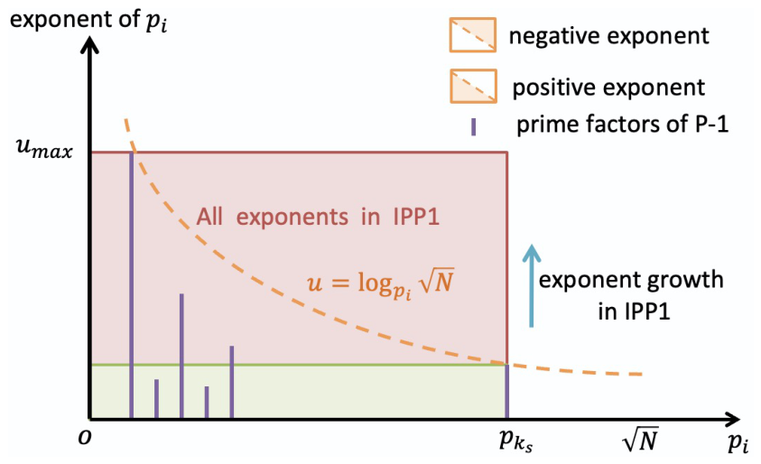
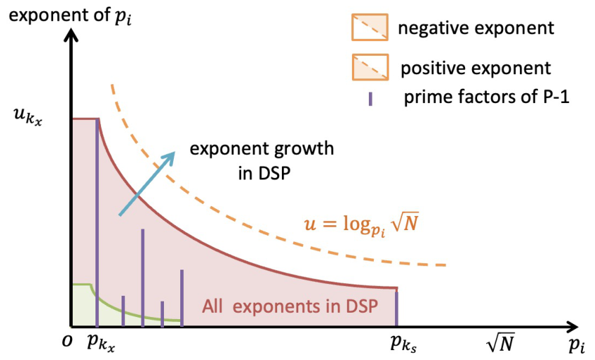
In $\mathsf{I}\mathsf{P}\mathsf{P}\mathsf{1}$, it selects a prime $p_t\ge p_{{\sigma }_s}$, then compute the product $z={\prod }_{i=1}^t{p}_i$ and iteratively calls a modular exponential operation at most $u_{\max }$ times to ensure all the prime factors for $P-1$ contained in $z^{u_{\max }}$. After that it can factor N by compute $\gcd (a^{z^{u_{\max }}},N)$ for a randomly chosen base a which is coprime to N. We can see that if $u_{\max }>{log}_{p_{{\sigma }_i}}\sqrt{N}$, then it produces an unnecessary overhead to calculate the exponent value for $p_{{\sigma }_i}$ in $\mathsf{I}\mathsf{P}\mathsf{P}\mathsf{1}$. Figure 5 shows such an overhead in the condition $u_{\max }>{log}_{p_{{\sigma }_s}}\sqrt{N}$. In our variant, we grow the exponents of each $p_i$ parallelly to the upper bound ${log}_{p_i}\sqrt{N}$ to avoid enumerating more invalid exponent as expressed in Figure 6 (more details about our variant can be seen in Section 3.1). The green part and red part denote the calculation amount for each $p_i$ and its exponent number $u_i$. The blue arrow implies that the calculation quantities in green part of $\mathsf{I}\mathsf{P}\mathsf{P}\mathsf{1}$ (Figure 5) or our variant (Figure 6) gradually grows to red part. The orange dash line can be considered to represent the calculation amount when the solution is successful. The variant solve the solution successfully only if the red part covers the orange dash line and all of its left area. It shows that our calculation amount is significantly lower than $\mathsf{I}\mathsf{P}\mathsf{P}\mathsf{1}$.

From the Theorem 1 and Theorem 2, the cost of finding the factor prime through our variant could be lower than $\mathsf{I}\mathsf{P}\mathsf{P}\mathsf{1}$ while $p_{{\sigma }_x}^{u_{{\sigma }_x}}<{\displaystyle \frac{1}{4}}{p}_{{\sigma }_s}^{{\displaystyle \frac{1}{2}}log{p}_{{\sigma }_s}+1}$. Since $p_{{\sigma }_x}^{u_{{\sigma }_x}}={max}_{1\le i\le s}{p}_i^{u_i}$, it infers that $p_{{\sigma }_x}^{u_{{\sigma }_x}}<P-1$. Since $p_{{\sigma }_s}>4$ in general, ${\displaystyle \frac{1}{4}}{p}_{{\sigma }_s}^{{\displaystyle \frac{1}{2}}log{p}_{{\sigma }_s}+1}>p_{{\sigma }_s}^{{\displaystyle \frac{1}{2}}log{p}_{{\sigma }_s}}$. We consider the probability of $p_{{\sigma }_s}^{{\displaystyle \frac{1}{2}}log{p}_{{\sigma }_s}}>P-1$ as $\mathrm{Pr}(p_{{\sigma }_s}^{{\displaystyle \frac{1}{2}}log{p}_{{\sigma }_s}}\ge P-1)=\mathrm{Pr}(p_{{\sigma }_s}\ge {(P-1)}^{{\displaystyle \frac{2}{log{p}_{{\sigma }_s}}}})=1-\mathrm{Pr}(p_{{\sigma }_s}<{(P-1)}^{{\displaystyle \frac{2}{log{p}_{{\sigma }_s}}}})=1-{\rho }_1({\displaystyle \frac{log{p}_{{\sigma }_s}}{2}})$, where $\rho$ function is defined in the page 162 of [13]. Suppose $p_{{\sigma }_s}\ge 64$, then ${\displaystyle \frac{log{p}_{{\sigma }_s}}{2}}\ge 3$. In page 163 of [13], it shows that ${\rho }_1\left(3\right)\le 0.05$ and ${\rho }_1$ is a monotonically decreasing function, so $\mathrm{Pr}(p_{{\sigma }_s}^{{\displaystyle \frac{1}{2}}log{p}_{{\sigma }_s}}\ge P-1)=1-{\rho }_1({\displaystyle \frac{log{p}_{{\sigma }_s}}{2}})\ge 0.95$ while $p_{{\sigma }_s}\ge 64$. Thus, $p_{{\sigma }_x}^{u_{{\sigma }_x}}\le P<{\displaystyle \frac{1}{4}}{p}_{{\sigma }_s}^{{\displaystyle \frac{1}{2}}log{p}_{{\sigma }_s}+1}$ in high probability while $p_{{\sigma }_s}>64$, i.e., our $\mathsf{DSP}$ algorithm is more efficiency than $\mathsf{I}\mathsf{P}\mathsf{P}\mathsf{1}$ in most of the time. Since $\mathsf{I}\mathsf{P}\mathsf{P}\mathsf{1}$ itself presets the size of B, it is expected that it will not set B below 64. In this case, even if the prime factors of $P-1$ are less than 64, our algorithm will still be faster.

5.2. Experimental Comparison Among 4 Variants of Pollard’s P-1 Algorithm

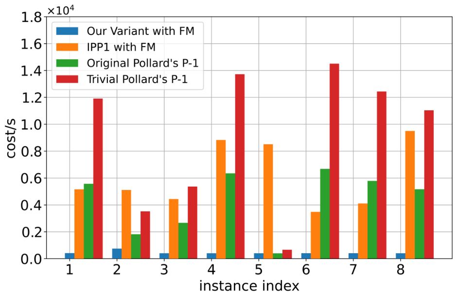
We’ve implemented Pollard’s P-1 algorithm in [3,5], $\mathsf{I}\mathsf{P}\mathsf{P}\mathsf{1}$ with fast multiplication technique as well as our variant (https://github.com/Summwer/expemeriment_of_pollardpm1, accessed on 1 August 2026). We design a prime generator to generate P so that $P-1$ is the product of several randomly generated 30-bit integers, which ensures the maximal prime factor of $P-1$ is the largest prime smaller than $2^{30}$. Then, we use the P to generate a random prime Q that in the same bit size of P and compute $N=PQ$. We test the above four algorithms in comparing the cost of factoring 10 entries of 1024-bit N, which was randomly generated by the above generator. We implement the test in a personal laptop (20.04.1-Ubuntu, x86-64, 6*Intel® Core™ i5-9500 CPU @ 3.00GHz, RAM 16 GB) with single thread. The experiment result is shown in Figure 7, we can see that our variant is around 23.5/16.4/35.6 times faster than the Algorithm $\mathsf{I}\mathsf{P}\mathsf{P}\mathsf{1}$/[3]/[5]. It shows that our algorithm has an absolute advantage in factoring an N with that the corresponding $P-1$’s factors have high exponents. In Figure 7, we can also find out that a randomly generated the product of several randomly generated 30-bit number has prime factors with high exponent (at least larger than 1) in high probability (instance 2,3,4,5,8). For some cases (instance 2,3,4,8), the $\mathsf{I}\mathsf{P}\mathsf{P}\mathsf{1}$ is slower than the original Pollard’s P-1, but in this case we are still faster than the original Pollard’s P-1. Since the multipliers in $P-1$ are chosen in randomly in Figure 7, it can be seen that the number of prime factors of $P-1$ or the size of the prime factor index have little impact on the complexity of our variant. Only the size of the largest prime factor is the only key influencing factor in our variant.

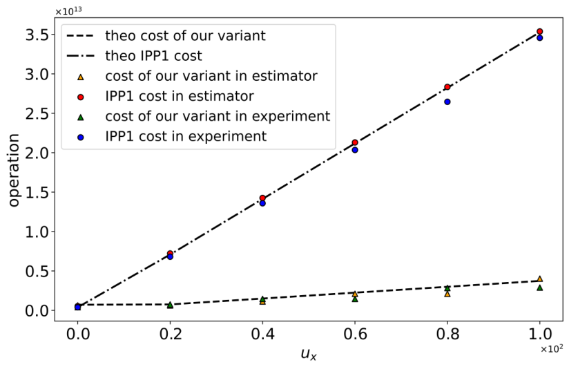
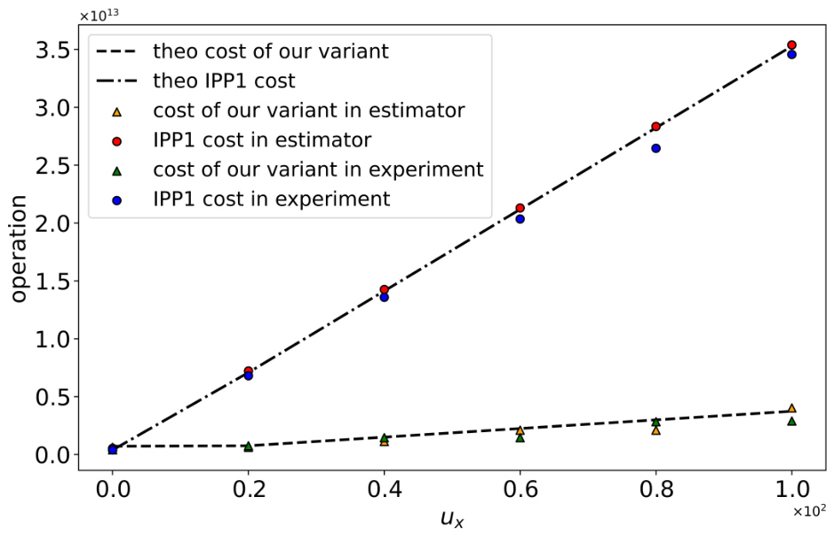
For the second experiment, we consider a situation that one prime factor of $P-1$ has a high exponent. We construct a 512-bit prime P in the form of $P=2\times 3^{u_x}\times 1073741789\times z+1$ ($u_x\in \{0,20,\cdots ,100\},$z is a number s.t. the larger entry $p^u|z$ satisfying $p^u<\min (3^{u_x},1073741789)$ for $p>3$) and a randomly 512-bit Q. Given $N=PQ$, we estimate the cost of our variant and $\mathsf{I}\mathsf{P}\mathsf{P}\mathsf{1}$ both in estimators (Algorithms 5 and 6) and the Theoretical Complexity Theorems (Theorems 1 and 2). We test the same instances in our variant (Algorithm 4) and $\mathsf{I}\mathsf{P}\mathsf{P}\mathsf{1}$ (Algorithm 3), Figure 8 shows that theoretical complexity fits well to the cost in both estimator and experiment.

6. Conclusions

We propose a variant of Pollard’s P-1 named Dynamic Scaling Pollard’s P-1 Algorithm. The proposed algorithm is an efficient method when all prime factors of $P-1$ or $Q-1$ are small. The proposed algorithm is quicker than previous Pollard’s P - 1 Algorithms for virtually all values of the modulus (especially $P-1$ has a prime factor with a high index), according to the experimental findings and the complexity analysis result. In factoring 1024-bit integer, our algorithm solves it nearly 23.5/16.4/35.6 times faster than the Algorithm $\mathsf{I}\mathsf{P}\mathsf{P}\mathsf{1}$ [6]/[3]/[5]. We also give a theoretical comparison between our $\mathsf{DSP}$ and $\mathsf{I}\mathsf{P}\mathsf{P}\mathsf{1}$, it concludes that our algorithm costs lower than $\mathsf{I}\mathsf{P}\mathsf{P}\mathsf{1}$ in more than 95% while the upper bound of prime list B in $\mathsf{I}\mathsf{P}\mathsf{P}\mathsf{1}$ is set to be larger than 64.

References

1. Rivest, R.L.; Shamir, A.; Adleman, L. A method for obtaining digital signatures and public-key cryptosystems. Commun. ACM 1978, 21, 120–126. [Google Scholar] [CrossRef] [Scilit]
2. Buhler, J.P.; Lenstra, H.W.; Pomerance, C. Factoring integers with the number field sieve. In The Development of the Number Field Sieve; Lecture Notes in Mathematics; Lenstra, A.K., Lenstra, H.W., Eds.; Springer: Berlin/Heidelberg, Germany, 1993; Volume 1554, pp. 50–94. [Google Scholar] [CrossRef] [Scilit]
3. Pollard, J.M. Theorems on factorization and primality testing. Math. Proc. Camb. Philos. Soc. 1974, 76, 521–528. [Google Scholar] [CrossRef] [Scilit]
4. Menezes, A.J.; van Oorschot, P.C.; Vanstone, S.A. Handbook of Applied Cryptography, 1st ed.; CRC Press: Boca Raton, FL, USA, 2018. [Google Scholar] [CrossRef] [Scilit]
5. Bishop, D. Introduction to Cryptography with Java Applets; Jones and Bartlett: Boston, MA, USA, 2003. [Google Scholar]
6. Somsuk, K. An Efficient Variant of Pollard’s p − 1 for the Case That All Prime Factors of the p − 1 in B-Smooth. Symmetry 2022, 14, 312. [Google Scholar] [CrossRef] [Scilit]
7. Avigad, J.; Donnelly, K.; Gray, D.; Raff, P. A formally verified proof of the prime number theorem. ACM Trans. Comput. Log. 2007, 9, 2. [Google Scholar] [CrossRef] [Scilit]
8. Ruckert, M.; Knuth, D.E. The Art of Computer Programming; Addison-Wesley: Upper Saddle River, NJ, USA, 2015. [Google Scholar]
9. Schönhage, A.; Strassen, V. Schnelle Multiplikation großer Zahlen. Computing 1971, 7, 281–292. [Google Scholar] [CrossRef] [Scilit]
10. Möller, B. Sliding Window Exponentiation. In Encyclopedia of Cryptography and Security; van Tilborg, H.C.A., Jajodia, S., Eds.; Springer: Boston, MA, USA, 2011; pp. 1222–1224. [Google Scholar] [CrossRef] [Scilit]
11. Corless, R.M.; Gonnet, G.H.; Hare, D.E.G.; Jeffrey, D.J.; Knuth, D.E. On the LambertW function. Adv. Comput. Math. 1996, 5, 329–359. [Google Scholar] [CrossRef] [Scilit]
12. Rabah, K. Review of Methods for Integer Factorization Applied to Cryptography. J. Appl. Sci. 2006, 6, 458–481. [Google Scholar] [CrossRef] [Scilit]
13. Riesel, H. Prime Numbers and Computer Methods for Factorization; Birkhäuser: Boston, MA, USA, 2012. [Google Scholar] [CrossRef] [Scilit]
Figure 1. Complexity comparison between our variant and IPP1 while bit ( N ) = 1024 , bit ( P ) = bit ( Q ) = 512 , where P 1 = 2 × 3 u x × 1073741789 , P and Q are both primes. The x-axis is u x and the y-axis is the cost in cycles. The green triangle is cost of our variant in experiment. The blue circle is the cost of IPP1 in experiment. The yellow triangle is the estimated cost of our variant generated by estimator. The red circle is the estimated cost of IPP1 generated by estimator. The dash line is the theoretical cost of our variant computed by Theorem 2. The dot-and-dash line is the theoretical cost of our variant computed by Theorem 1.
Cryptography 10 00057 g001
Figure 2. Optimal w to minimize 2 w 1 1 + l 1 w + 1 .
Cryptography 10 00057 g002
Figure 3. Simulation of f ( w ) min = min 1 w l 2 w 1 1 + l 1 w + 1 which shows that the function f ( w ) min fits well with a linear function.
Cryptography 10 00057 g003
Figure 4. Experimental result of normal multiplication method and FM. The red star point (orange point) is the experimental cost of normal/fast multiplication method, which computes the cost of all primes smaller than or equal to the bit size shown in x-coordinate. The gray (red) dashed line is the theoretical cost of normal/fast multiplication method. It fits the experimental result, which means that the theoretical analysis is correct.
Cryptography 10 00057 g004
Figure 5. Exponent growth in [6]. The x axis is the prime number, the y axis means the exponent value of each prime. The purple line shows a sample with the prime factors and its exponent number of P 1 . The blue arrow denotes the growth direction for adding new prime factors in I P P 1 . The orange line means the representation of u = log p i N . If the index value exceeds the orange line, it means that we increase the extra index of the prime factor p i . The red block means the minimal scope to add prime numbers through I P P 1 .
Cryptography 10 00057 g005
Figure 6. Exponent growth in our variant. The x axis is the prime number, the y axis means the exponent number of each prime. The purple line shows a sample with the prime factors and its exponent number of P 1 . The blue arrow denotes the growth direction for adding new prime factors in our variant. The orange line means the representation of u = log p i N . If the index value exceeds the orange line, it means that we increase the extra index of the prime factor p i . The green block indicates the steady incremental allocation of exponents that drives the DSP cost toward its asymptotic scaling. The red block means the minimal scope to add prime numbers through our variant.
Cryptography 10 00057 g006
Figure 7. Practical cost for our variant (blue one), I P P 1 (orange one), Original Pollard’s P-1 Algorithm [3] (green one) and Trivial Pollard’s P-1 Algorithm [5] (red one) to factor an 1024-bit N. The x-axis is the index for the randomly generated instance. The y-axis is the cost in second.
Cryptography 10 00057 g007
Figure 8. The figure shows growth accuracy for DSP and I P P 1 with a 1024-bit N and 512-bit primes P, Q with P 1 = 2 × 3 u x × 1073741789 ; the x-axis is u x and the y-axis is cost in cycles. Experimental results are marked by green triangles ( DSP ) and blue circles ( I P P 1 ), estimator predictions by yellow triangles ( DSP ) and red circles ( I P P 1 ), while theoretical costs are given by a dashed line ( DSP , Theorem 2) and a dash-dotted line ( I P P 1 , Theorem 1).
Cryptography 10 00057 g008