Enhancing Malignant Lymph Node Detection in Ultrasound Imaging: A Comparison Between the Artificial Intelligence Accuracy, Dice Similarity Coefficient and Intersection over Union

Abstract

Background: The accurate identification of malignant lymph nodes in cervical ultrasound images is crucial for early diagnosis and treatment planning. Traditional evaluation metrics, such as accuracy and the Dice Similarity Coefficient (DSC), often fail to provide a realistic assessment of segmentation performance, as they do not account for partial overlaps between predictions and ground truth. This study addresses this gap by introducing the Intersection over Union (IoU) as an additional metric to offer a more comprehensive evaluation of model performance. Specifically, we aimed to develop a convolutional neural network (CNN) capable of detecting suspicious malignant lymph nodes and assess its effectiveness using both conventional and IoU-based performance metrics. Methods: A dataset consisting of 992 malignant lymph node images was extracted from 166 cervical ultrasound scans and labeled using the ImgLab annotation tool. A CNN was developed using Python, Keras, and TensorFlow and employed within the Jupyter Notebook environment. The network architecture consists of four neural layers trained to distinguish malignant lymph nodes. Results: The CNN achieved a training accuracy of 97% and a validation accuracy of 99%. The DSC score was 0.984, indicating a strong segmentation performance, although it was limited to detecting malignant lymph nodes in positive cases. An IoU evaluation applied to the test images revealed an average overlap of 74% between the ground-truth labels and model predictions, offering a more nuanced measure of the segmentation accuracy. Conclusions: The CNN demonstrated high accuracy and DSC scores, confirming its effectiveness in identifying malignant lymph nodes. However, the IoU values, while lower than conventional accuracy metrics, provided a more realistic evaluation of the model’s performance, highlighting areas for potential improvement in segmentation accuracy. This study underscores the importance of using IoU alongside traditional metrics to obtain a more reliable assessment of deep learning-based medical image analysis models.

1. Introduction

Cervical lymph nodes play a crucial role in the immune response, but their enlargement can indicate a wide range of pathological conditions, spanning from benign reactive hyperplasia to malignant metastases. Differentiating between benign (inflammatory and/or infectious) and malignant lymphadenopathies is essential for early diagnosis and appropriate treatment planning [1]. The head and neck region alone contains more than 300 nodes [2]. Studies have shown that patients with nodal metastases have a 50% lower five-year survival rate, dropping to below 25% when the malignancy spreads bilaterally [3].

Lymph node metastasis is a key factor in determining head and neck cancer prognoses. Upon discovery, these nodes provide information regarding the localization of the primary tumor, indicating a higher likelihood of its presence in the head and neck region [4]. Also, most frequently, the malignant lymph nodes underline the presence of a distant metastasis from a hidden nasopharyngeal carcinoma [5]. Given the overlap in clinical presentation, physical examination alone is often insufficient, thus necessitating the use of imaging modalities such as ultrasound (US), computed tomography (CT), and magnetic resonance imaging (MRI). Among these, US is preferred due to its real-time evaluation capabilities, non-invasiveness, and cost-effectiveness, making it the primary imaging tool for initial assessments of lymph node characteristics. This procedure can also support puncture biopsy, providing a definitive anatomopathological result [6]. A recent study involving 235 patients and 4539 ultrasound-evaluated lymph nodes compared ultrasound imaging findings with histopathological results, confirming that ultrasound remains the most effective imaging modality for detecting lymph node metastases [7].

High-resolution US offers high sensitivity (97%) and specificity (93%) when confirmed with fine-needle aspiration [8]. The gray-scale sonographic features include a larger size, a round shape (with a long axis/short axis ratio lower than 2), being predominantly hypoechoic with a heterogeneous echotexture, and the absence of the central (hyperechoic) hilum [9]. Moreover, Doppler ultrasound can also contribute since malignant lymph nodes are more likely to have a peripheral signal. US elastography has proven useful in the early detection of both cortex and medullar stiffness [10]. However, the Doppler and elastography windows are not included in this study.

In this study, we pursued two objectives: first, we aimed to develop a convolutional neural network (CNN) capable of identifying suspicious malignant lymph nodes; second, we aimed to compare a traditional accuracy metric, the Dice Similarity Coefficient (DSC), and the Intersection over Union (IoU) to prove that the latter offers a more precise assessment of the network’s performance. This comparison is crucial for avoiding the bias of high accuracy in small datasets and ensuring a more accurate assessment of model performance. By addressing this bias and providing a clear understanding of the true performance of networks, we aim to inspire the confidence necessary for their adoption in hospital settings.

Although no one sonographic parameter can give rise to a clear certainty of malignancy, there are specific characteristics (in gray-scale and Doppler) that can guide diagnosis, as previously described [11]. To achieve the objectives mentioned above, we decided to use only gray-scale images for training, although when we selected the patients for the database, we also consulted the Doppler and elastography features of the corresponding US machine. Gray-scale-suspicious characteristics of the lymph nodes include a larger size, roundness (or a ratio between the long and short axes of less than 2), being predominantly hypoechoic with a heterogeneous echo-structure, ill-defined margins, and the absence of the central (hyperechoic) hilum. There may also be microcalcifications, necrosis, or other typical features derived from the primary tumor [12].

The conventional accuracy used to evaluate the performance of a CNN is measured by comparing the predicted labels (of the program used) with the labels from the dataset. Mathematically, this represents the ratio of the number of correct predictions multiplied by 100 to the total number of predictions. However, the labels do not have to fully overlap to be considered a correct prediction because this type of accuracy focuses on the overall correctness rather than pixel-level correspondence [13].

The DSC or F1 is a statistical tool used to compare the similarity of two samples [14]. There has been interest in applying Dice’s Coefficient in image segmentation since 1994 [15].

The IoU or Jaccard is an evaluation metric that compares labels with the predictions generated by a program. This method is used in object detection and image segmentation AI programs. The IoU is determined using the following formula: Area of Overlap/Area of Union. It has a score ranging from 0 to 1 [16].

Studies have explored the segmentation abilities of various neural networks. In the context of ultrasound imaging, a recent study focused on automatic detection by comparing the performance of well-established CNNs, such as YOLOv4, with a custom-designed network for detecting foreign objects in neurosurgery. The results varied depending on the network architecture, with the custom model achieving the highest performance, attaining a median IoU of 94% in detecting cotton balls [17]. Another study, conducted on breast US images, reported that a median IoU of 82.83% was achieved for the corresponding dataset [18].

The main contributions of this study are as follows: we developed a CNN trained for detecting cervical malignant lymph nodes in US images and compared the conventional accuracy with DSC and IoU to provide a comprehensive evaluation of segmentation performance. Through the mentioned comparison, we aim to demonstrate that IoU offers a more realistic assessment of model performance, highlighting its importance in future deep learning applications for medical imaging.

2. Materials and Methods

A database consisting of images of 220 patients (8540 B-mode images) was analyzed. The patients selected underwent cervical US imaging via a Sonoscape S2 (2012) Portable US Machine between 2012 and 2023. The database was anonymized by refraining from saving patient information during the investigation. Codes randomly generated by the US machine were used. The images were analyzed by a team consisting of 1 ENT physician, 1 radiology physician, and 1 nuclear medicine resident. According to the inclusion criteria, the patients included in this study had to have at least one suspicious lymph node image, the images had to be clear, and all 3 physicians had to agree on the presence of the lymph node in the selected image. The exclusion criteria consisted of blurred images, the presence of annotation (such as dimensional axes), and Doppler signal or elastography windows. Although these features are important, we chose to exclude the Doppler and elastography windows due to the limited number of cases containing both, as their inclusion would have significantly reduced the dataset and led to a lack of normal images. After applying the criteria, a total of 53 patients (166 images) were chosen. From the 166 images obtained, 150 were selected to augment the data for training and validation, while 16 were kept original for testing. The remaining 150 training images were then cut using the original bounding boxes to obtain positive and negative images (with lymph nodes and without lymph nodes) with dimensions of 100 × 100 in order to train the neural network. This process led to a total of 1732 small, 100 × 100 images either containing a full-size lymph node or a background of the main image.

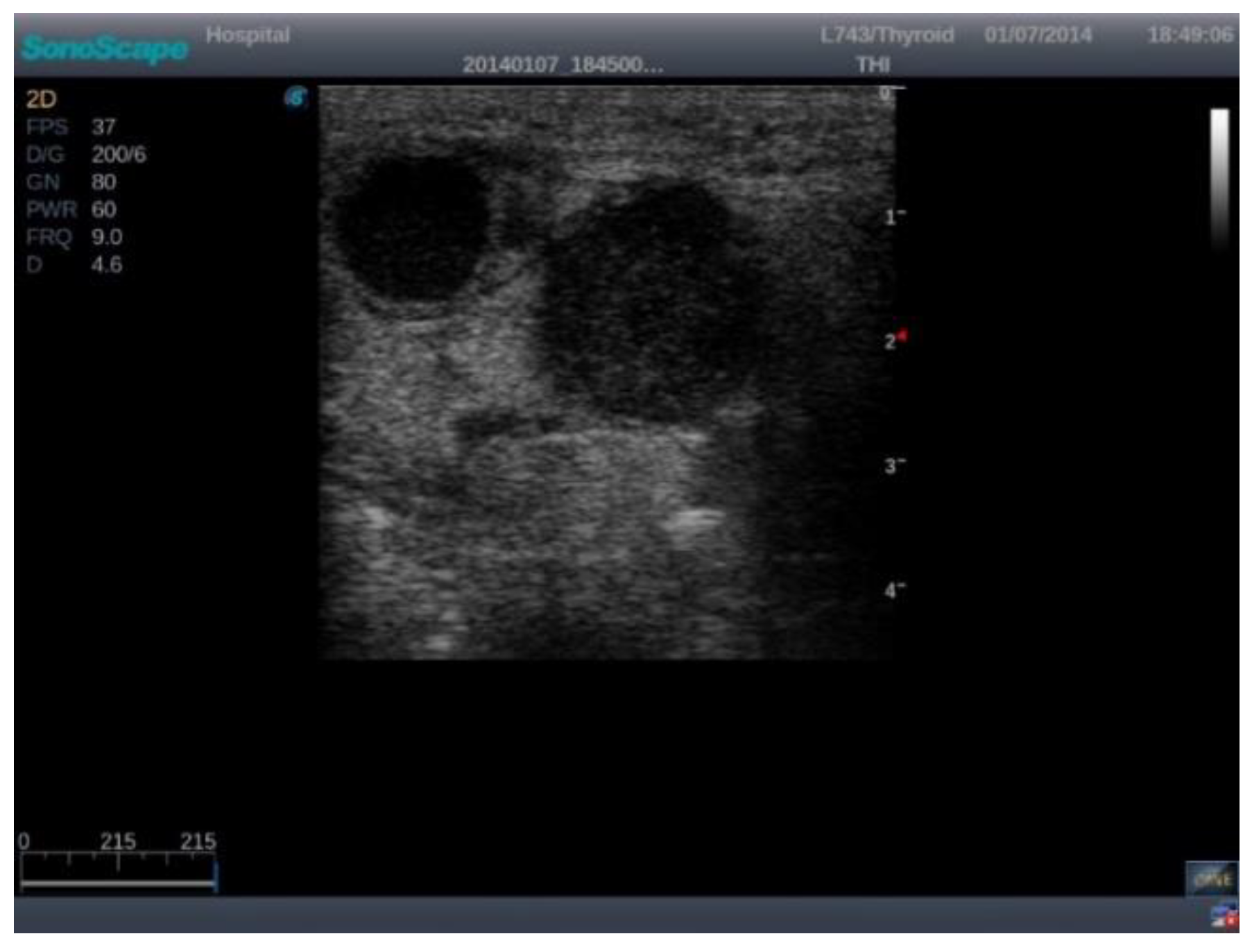
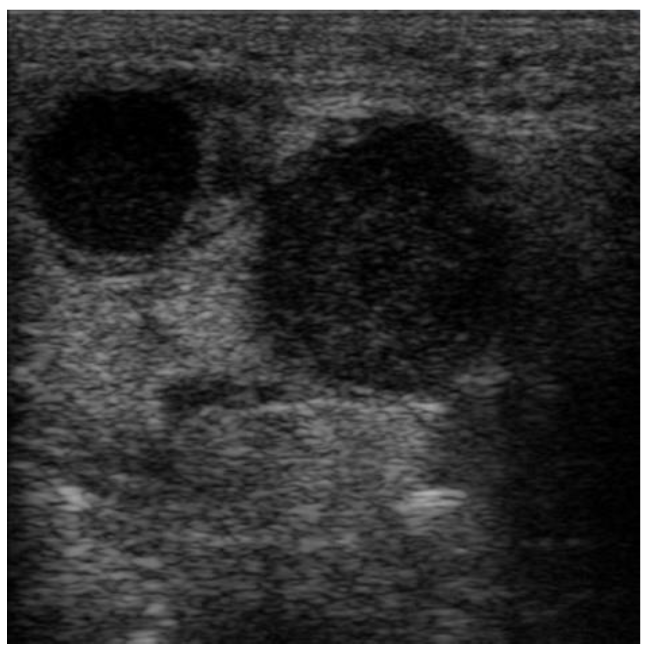
The images were exported from the device used in .jpg format (Figure 1) directly from the US machine and processed by cropping them and resizing them to 469 × 469 pixels (Figure 2).

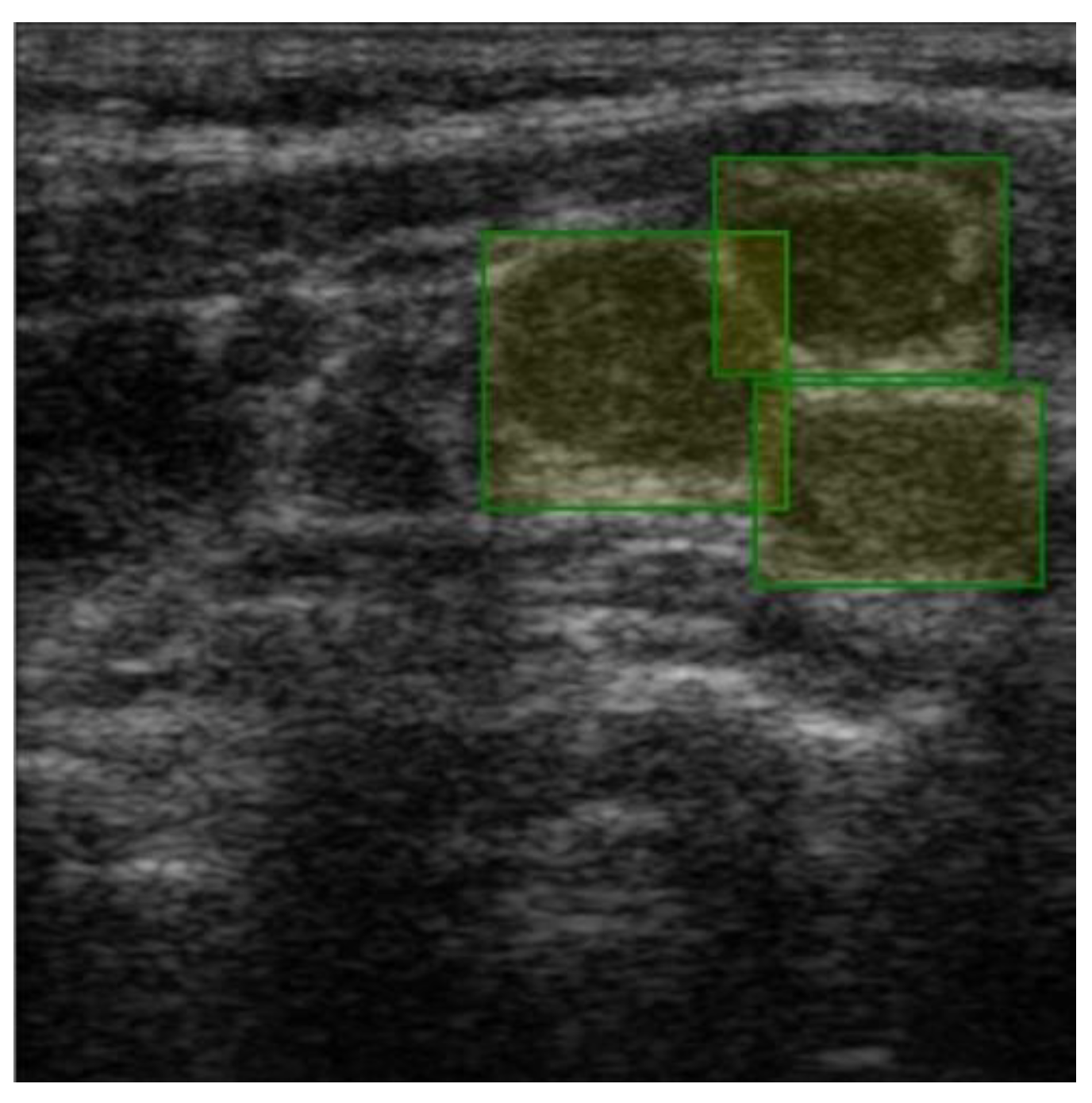
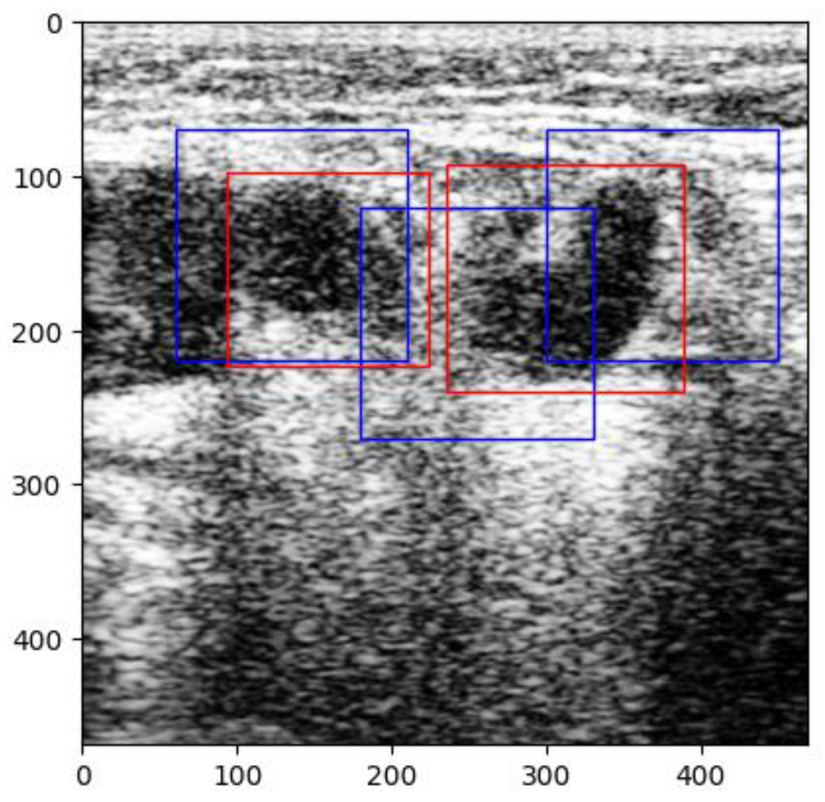
Labeling was conducted using a free online tool (ImgLab) (Figure 3). The labels were made by the team of physicians that selected the images. Overlapping labels were not a problem for our neural network because the lymph nodes were individually cropped. Therefore, the lymph node images within an adenopathic block were all labeled individually (Figure 4). The labels were saved in .json file format.

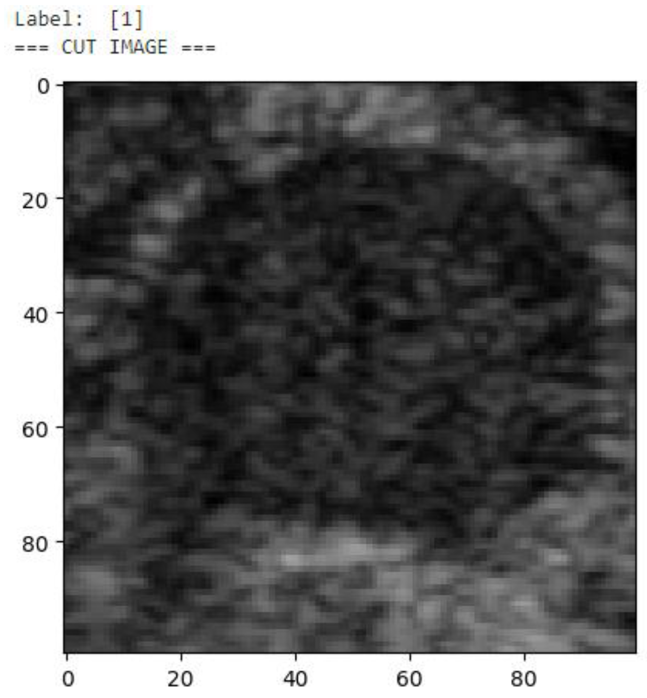
After the images were labeled, each malignant ganglion was cropped separately into a new image to augment the number of images in the training and validation sets (Figure 5). Then, each of these images was used to generate 3 more images through rotation and flipping, resulting in a final dataset consisting of 992 images of malignant lymph nodes (Figure 6). To train the network properly, we also required examples of boxes without lymph nodes. Given the input image and the bounding boxes, smaller 100 × 100-pixel images were cut from the original image to obtain small images with and without lymph nodes. Thus, we cropped 740 images without any lymph nodes. As a normalization technique, to obtain pixel values between 0 and 1, the pixel matrix of each image was divided by 255 before being added to the training and validation dataset. The same division process was applied for the testing images before they were input into the trained neural network before the predictions were made. The small images (100 × 100) were flipped horizontally and vertically to obtain more images from the dataset. The resulting 1736 small images were then split into training and validation datasets using a built-in Keras function, resulting in a training set consisting of 1562 images (with and without lymph nodes) and a validation dataset consisting of 174 images (with and without lymph nodes). Each new image was labeled as ‘1’ if it contained a malignant lymph node and ‘0’ if it did not. Moreover, the images were shuffled to randomize the order in which the characteristics were presented to the CNN during training.

To implement the code, we utilized the Python (3.11) programming language due to its efficiency in neural network development, along with the Keras and TensorFlow libraries. For the coding environment and model training and testing, we used Jupiter Notebook provided by the Kaggle platform. Kaggle offers its users free access to NVIDIA TESLA P100 GPUs, with a limit of approximately 30 h per week. The general hardware specifications include Intel Xenon CPUs (2.3 GHz, 16 cores) and 13 GB of RAM.

A convolutional neural network architecture was chosen to obtain the results. A neural network is a set of ‘neurons’, which are no more than numerical parameters that must be set during a training session. The convolution process is just a multiplication operation between the value of the pixels in the images and the trained parameters. The result of the convolution is subjected to the activation function, which decides if the information contained in these pixels is valuable enough for the output of the neural network. In the end, after more convolution operations that are ‘verified’ by the activation functions, a numerical result is obtained, which, in our case, can be either close to 0 (denoting the absence of malignant adenopathy) or close to 1 (denoting the presence of a malignant lymph node). In order to be as precise as possible, only the results with a confidence of over 95% are represented as the output.

The aim of the training process is to set the parameters of the CNN. The information flows through the network and, in the end, is compared with the reference data (the la-bels decided by the specialists). If the predicted results are too far from the desired result, the loss function penalizes the neural network, which then has to adapt its parameters to obtain values closer to the real ones. This is an iterative process, which, in our case, was carried out 20 times.

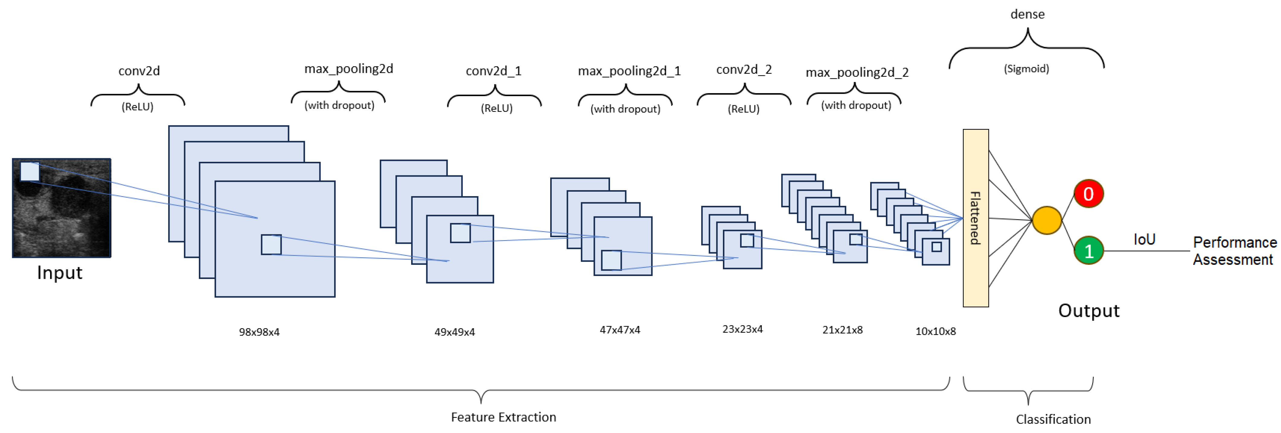
Our neural network consists of 4 layers (

Table 1. The CNN layer structure used.

Layer (Type)	Output Shape	Parameter #
conv2d (Conv 2D)	(None, 98, 98, 4)	112
batch_normalization (BatchNormalization)	(None, 98, 98, 4)	16
activation (Activation)	(None, 98, 98, 4)	0
max_pooling2d (MaxPooling 2D)	(None, 49, 49, 4)	0
dropout (Dropout)	(None, 49, 49, 4)	0
conv2d_1 (Conv 2D)	(None, 47, 47, 4)	148
batch_normalization_1 (BatchNormalization)	(None, 47, 47, 4)	16
activation_1 (Activation)	(None, 47, 47, 4)	0
max_pooling2d_1 (MaxPooling 2D)	(None, 23, 23, 4)	0
dropout_1 (Dropout)	(None, 23, 23, 4)	0
conv2d_2 (Conv 2D)	(None, 21, 21, 8)	296
batch_normalization_2 (BatchNormalization)	(None, 21, 21, 8)	0
activation_2 (Activation)	(None, 21, 21, 8)	0
max_pooling2d_2 (MaxPooling 2D)	(None, 10, 10, 8)	0
dropout_2 (Dropout)	(None, 10, 10, 8)	0
flatten (flatten)	(None, 800)	0
dense (Dense)	(None, 1)	801

and Figure 7). The layers used to assemble the neural network are as follows:

1. Batch normalization—This layer applies a transformation to normalize the inputs. It is an optional layer that accelerates training, improves stability, and reduces overfitting [19].

2. Activation—This layer manages the neuron output in a neural layer by using a mathematical function. Our first 3 layers use the ‘Rectified linear unit’ (ReLU), while the 4th layer uses the ‘Sigmoid’ [20].

3. Max pooling—This layer selects the maximum value for each region of the input feature map in order to reduce overfitting, accelerate training, and help reduce the spatial dimensions [21].

4. Dropout—During each training step, a certain percentage of nodes in a layer are randomly ignored in order to prevent overfitting and promote robustness [22].

In the training process, we obtained the best results using the following parameters: a batch size of 5 and 20 epochs. The loss function also plays a fundamental part in the training process, as it quantifies the differences between the predicted and actual values. In our program, we used binary cross-entropy loss (Equation (1)), which is usually used for 0–1 classification. To make the predictions closer to the ground-truth values, an optimizer must be used. For our application, we decided that the ‘adaptative moment estimation’ (Adam) optimizer would be best since it covers a variety of neural network projects and has been proven to offer reliability and good performance. After several experiments, the learning rate was set to 0.0001 so that the network would converge to a solution more slowly, allowing it to learn more details about the texture of the training images.

No specific function was used to initialize the model weights prior to training. Although it is known that small random weights are recommended for the beginning of training, given the low complexity of the task, no weight initialization methods were used.

$$-(y log (p)+(1-y\left)log\right(1-p)$$

(1)

3. Results

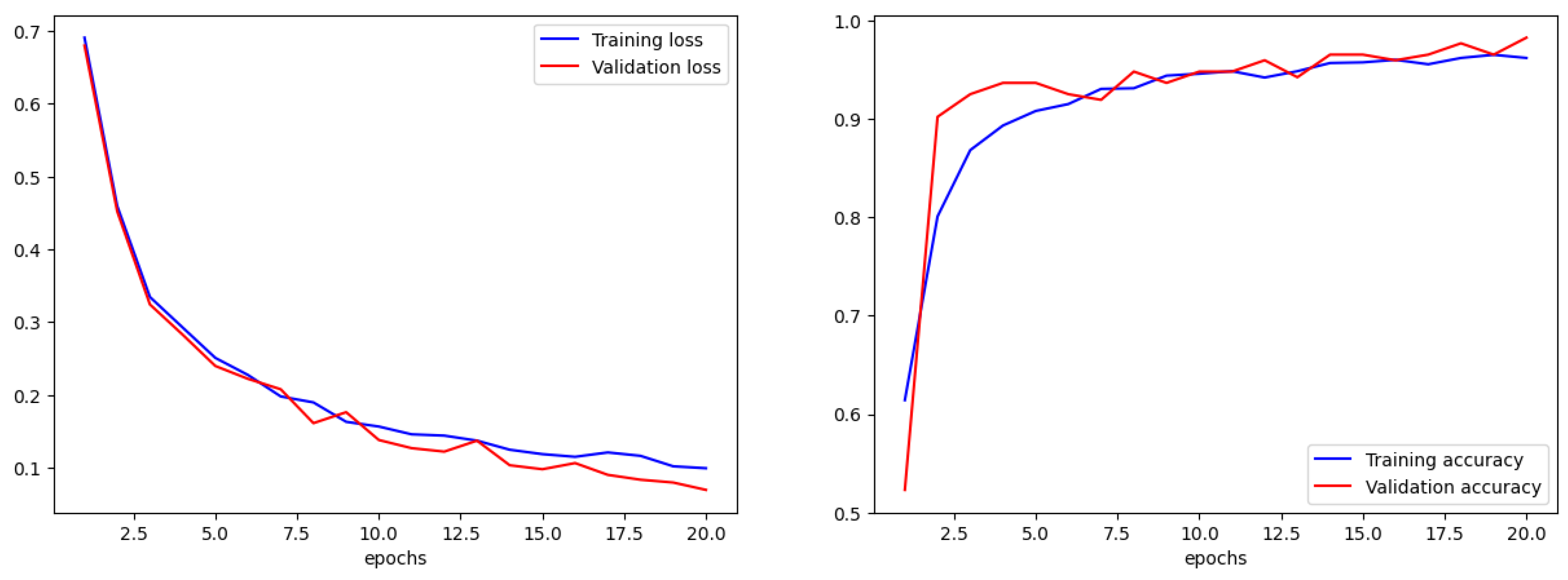
We compared the training accuracy with the validation accuracy in terms of accuracy and error. For a correct training process, the trends in validation and training must be similar. If the training parameters are not adjusted correctly, there will be an obvious difference between them. The overall accuracy for the training set was 97% with a loss (error) of 0.1, while the validation accuracy was 99% with a loss of 0.07 (Figure 8).

The formula for accuracy is given below in Equation (2).

$$\mathrm{Accuracy}=\frac{\mathrm{Number} \mathrm{of} \mathrm{Correct} \mathrm{Predictions}}{\mathrm{Total} \mathrm{Number} \mathrm{of} \mathrm{Predictions}}$$

(2)

Afterwards, we applied the DSC formula (Equation (3)). Surprisingly, the score was 0.984, which translates into 98% performance, but in our case, it did not verify the percentage of overlap between the label and the prediction. Instead, it only evaluated the ability to detect malignant lymph nodes in images that are positive.

$$DSC=2 \ast {\displaystyle \frac{\Sigma \left(\mathit{\text{validation\_predictions}}\right)}{\left(\Sigma \right(\mathit{\text{validation\_predictions}})+\Sigma (\mathit{\text{y\_val}}\left)\right)}}$$

(3)

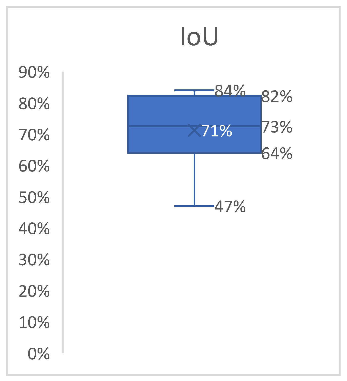
Since our goal was to determine the overlap ratio between the predictions and the labels made by the experts in the field, we searched for alternative ways of reaching our objective, so we applied another metric, IoU. The formula used to calculate IoU is presented in Equation (4) [23]. The better the alignment between the predictions and the label, the more accurate the network. 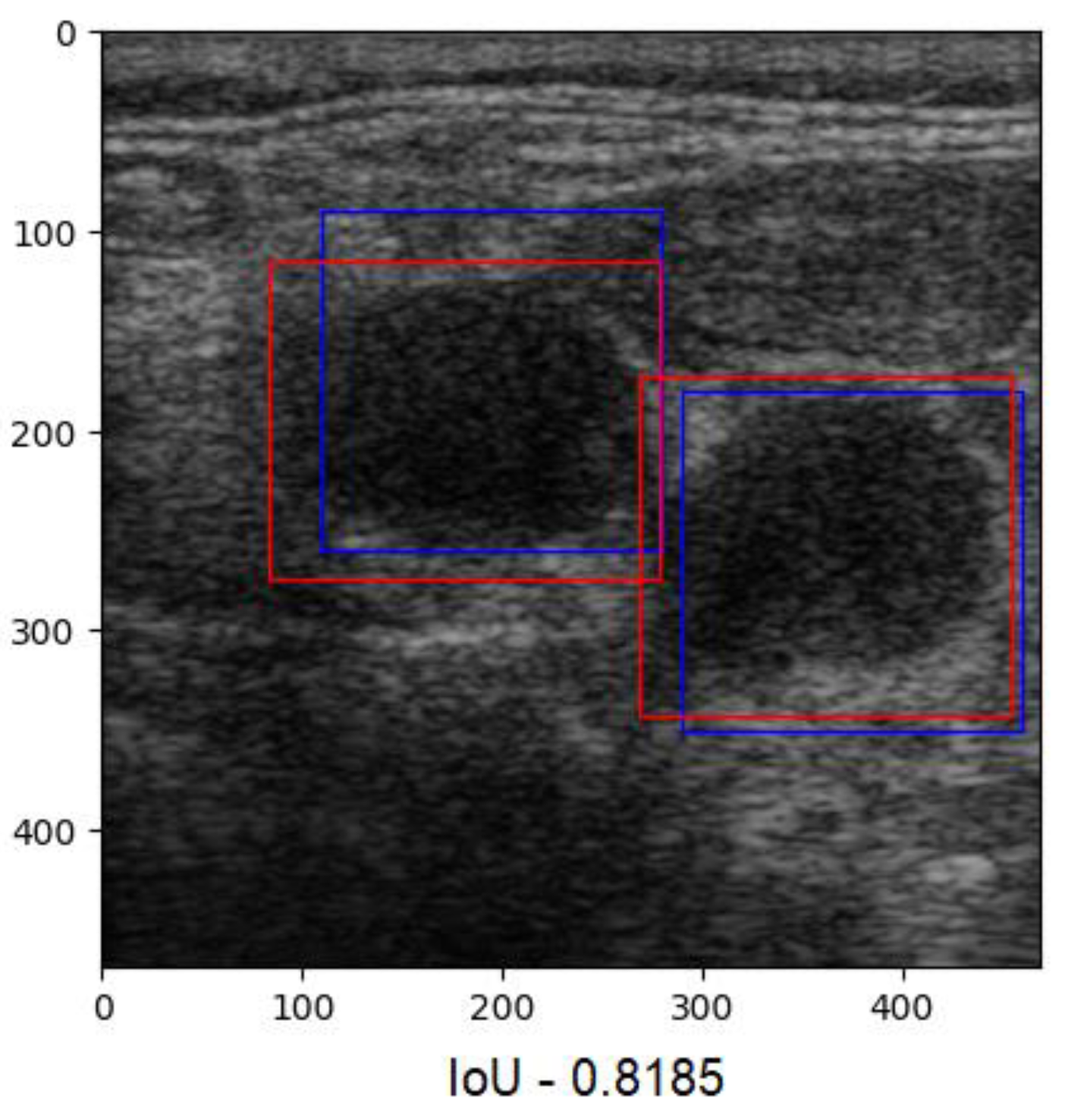Since this technique verifies each label individually, we averaged the results into a boxplot (Figure 9). The overlap ratio between the predictions and labels ranged between 47% and 84% on the test images, with an average of 74%. Few aberrant labels were ignored. One of the final predictions can be seen in Figure 10.

$$IoU={\displaystyle \frac{Area of Overlap }{\mathrm{A}\mathrm{r}\mathrm{e}\mathrm{a} \mathrm{o}\mathrm{f} \mathrm{U}\mathrm{n}\mathrm{i}\mathrm{o}\mathrm{n}}}$$

(4)

Accuracy and the DSC reveal the network’s ability to determine whether a given image contains a lymph node, while the IoU indicates the overall program’s ability to determine the location of the ganglion in an image. High accuracy and DSC values assure the user that a given image will be correctly labeled, and a high IoU value assures the user that the overall program will be able to find the region of interest in an image.

Unlike other studies, wherein a combination of algorithms, such as YOLOv8 and MobileViT, along with a mountaineering-team-based optimization technique, was employed to enhance segmentation and feature extraction (as reported in a study regarding mandibular condyle detection [24]), our approach is more straightforward, using label coordinates to generate the ground-truth segmentation maps.

The output shape of the CNN is a one-dimensional vector consisting of values either close to 0 or close to 1. This vector is input into the DSC metric along with the ground-truth vector, which is also a one-dimensional array. Subsequently, the sliding window function, which takes the ultrasound image as an input, creates slices from it that are exactly the size that the CNN expects. These slices are labeled by the CNN as either containing a lymph node or not. Afterwards, the slices containing the lymph nodes are overlapped with the ground-truth boxes labeled by the experts to assess the percentage of the overlap between the two.

To sum up, our network’s output is a vector suitable for computing accuracy and the DSC (a one-dimensional binary classification array), labeling slices from the original ultrasound image as containing a lymph node or not. If a slice contains a lymph node, then this slice’s coordinates are used for IoU computation.

Our results are comparable to those reported in other state-of-the-art studies on this topic, though the mean IoU value was slightly lower, as expected. A recent study published in 2024 explored the use of deep learning to assist in the diagnosis of cervical lymph node metastasis in patients with thyroid cancer. This study reported an accuracy of 72% and a mean DSC of 0.832, calculated from labels and prediction areas, with a similar formula for IoU [25]. The difference is that the IoU metric generally penalizes individual instances of poor classification more severely than the DSC, even though both of them recognize when an instance is misclassified. As a result, the IoU metric tends to amplify the impact of errors to a greater degree compared to the DSC [26].

A study on a machine learning algorithm designed to grade facioscapulohumeral muscular dystrophy using musculoskeletal ultrasound images trained on a dataset consisting of 25,005 images achieved comparable results, reporting an IoU of 74.03% [27].

An interesting perspective on the diagnosis of unexplained cervical lymphadenopathy was found in a recent paper that aimed to develop a deep learning radiomics model for assisting radiologists. The NN was trained on both B-mode and color Doppler images and integrated three sub-models together. The cited study provided accuracies for the three sub-models individually, varying with the cohorts between 75.8% and 87.6% in differentiating benign and malignant unexplained cervical lymphadenopathies [28]. There was no information on the DSC or IoU, but heatmaps were applied for interpreting the hybrid decision-making network, and, overall, it increased the diagnostic accuracies of young radiologists.

Another study whose aim was to develop a deep learning algorithm to predict cervical lymph node metastases from primary thyroid cancer using US images obtained an accuracy of 0.79 on the test set. The DSC (F1) score was also 0.79 [29]. The DSC formula was not explicitly provided, but it was likely applied in a manner consistent with our approach.

Deep learning was utilized to predict late cervical lymph node metastasis in tongue cancer using US B-mode images. The dataset comprised 37 images from 22 patients with occult cervical lymph node metastasis and 52 images without metastasis. To expand the dataset, image augmentation techniques, such as rotation and flipping, were applied, resulting in a final dataset consisting of 142 images with metastatic lymph nodes. The accuracy achieved was 79.8% [30]. Leveraging the sliding window technique, we were able to augment our data by rotating and flipping each lymph node individually, thereby increasing the number of examples for our CNN, as reflected in our metrics.

In 2022, a group of researchers aimed to develop an automated classification system for cervical lymph nodes detected via ultrasound. The dataset was extensive, comprising 2268 US images from 1146 patients. Several neural network models were tested, yielding accuracies ranging from 69.85% to 78.53% and mean DSC overlap values ranging from 68.46% to 77.19% [31]. As previously mentioned, accuracy reflects an NN’s performance in terms of classification ability. Unlike our approach, which focuses solely on identifying malignant lymph nodes, their NN classified lymph nodes as either benign or malignant. This distinction may account for the differences in accuracy between our research and theirs, despite our use of data augmentation, which was not employed in their study. While our supposition regarding the difference in accuracy being due to the classification tasks and data augmentation is plausible, several factors could influence the results, including differences in model architectures, training processes, and evaluation metrics. Thus, these elements should be considered when interpreting the results and comparing them with our study.

A recent systematic review explored studies published between 2001 and 2022 regarding the application of AI to classify cervical lymph nodes. Unfortunately, data pertaining to the use of ultrasound as an imaging method were not included in this paper. However, the studies (conducted on CT, MRI, or PET/CT images) had a mean of 75 patients included, with a range of between 10 and 258. The accuracies ranged from 43% to 99% for the training sets and 76% to 92% for the testing sets. None of the cited studies explored using the DSC or IoU to assess the performance of the corresponding NN [32]. Using a retrospective dataset (consisting of 185 images), the authors of another study aimed to develop a deep learning-based computer-aided diagnosis method. The model used obtained accuracies of 86.3% on a retrospective dataset and 92.4% on a prospective test set [33]. Another review study analyzed the performance of some AI programs developed to identify metastatic lymph nodes in patients with head and neck squamous cell carcinoma. In terms of performance, the programs’ accuracies ranged from 43 to 99% [32]. Using the YOLOv7 CNN, metastatic lymph nodes were identified with an accuracy of 81% on the validation set, which is greater than the results for residents (66%) [34].

4. Discussion

Our initial approach was to use the entire image, provide the program with the box coordinates of the label (the malignant lymph node), and then allow it to search for specific characteristics.

This test was conducted on 166 images, using 150 images for training and 16 for testing. Unfortunately, the program was not able to identify any lymph nodes adequately. The measured accuracy was around 60%, with a high loss value (0.4). One of the main reasons seemed to be due to the small dataset employed. Additionally, it was not possible to attach multiple tags to each lymph node in an image.

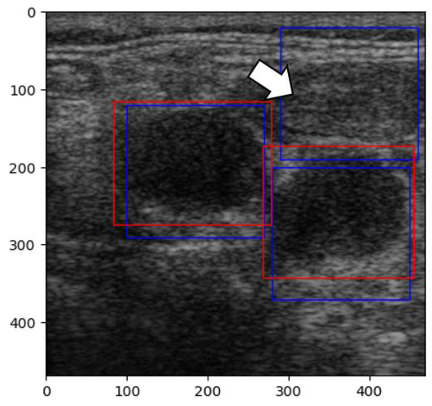
In our second attempt, we rebuilt the CNN using the sliding window technique. The sliding window technique involves moving a fixed or variable-size window through a data structure (an image, in our case) to efficiently solve problems involving continuous subsets of elements. This method efficiently identifies specific criteria present in data [35]. The images were pre-processed by normalizing the pixels’ values between 0 and 1. With this new technique, new challenges arose because of prediction overlap, which prevented us from correctly calculating the IoU between labels and predictions (Figure 11).

Another change we made to increase performance concerned the number of images without lymph nodes. Initially, the program was given 224 images without malignant lymph nodes for training. As noted previously, this number was increased to 740 images, thus providing more examples of non-malignant lymph nodes. Nevertheless, the program still occasionally raised suspicion of malignant adenopathy on some muscles in the axial plane (Figure 12), which brings us to the discussion of the false positive and false negative results obtained by our CNN. Naturally, this network is not flawless, and some false positive and false negative results were provided. Understanding the implications of false positives and false negatives is crucial when evaluating the performance of a CNN. False positives occur when a model incorrectly classifies an anatomical structure as a malignant lymph node (which can lead to unnecessary investigations or patient anxiety), while false negatives are instances where a malignant lymph node is present in an image but remains unrecognized by the network. Although the network is no more than a binary classifier, it is embedded in an object detection algorithm that uses bounding box coordinates to predict results. For binary classification, the confusion matrix was computed over the 174 validation images. The results are presented in

Table 2. Confusion matrix on the validation set.

	Actually Positive (1)	Actually Negative (0)
Predicted to be Positive (1)	63	1
Predicted to be Negative (0)	13	97

.

One observed instance of a false positive in our tests involved the misclassification of the sternocleidomastoid muscle in axial planes as a malignant lymph node. The model appeared to be predisposed to confusing these structures due to their similar echogenic characteristics (Figure 12).

In one instance, the model was unable to detect two small malignant lymph nodes present in the same image, likely due to their size and echogenicity. This implies that certain subtle characteristics and variations were not adequately learned by the CNN, most likely because of limited diversity in the training dataset.

In one of our previous manuscripts, we analyzed and described some results obtained in different studies regarding AI programs applied in the ENT field. Most of the AIs were trained on CT and IRM images, using different types of CNNs. The accuracies obtained in these studies varied between 70% and 98% [36].

The application of deep learning in US imaging became a subject of interest because imaging analysis might be the key to improving both the volume and the precision of pathological evaluations [37]. Some studies report similar performances of these algorithms even when compared to radiologists’ evaluations [38], while others have reported that such algorithms helped young physicians improve their diagnostic accuracy. However, regarding malignant cervical lymph nodes, the studies are limited, as presented above.

There have been multicentric studies focused on developing AI programs capable of detecting malignant adenopathy in patients with breast cancer. The sensitivities obtained were around 94%, while the specificity was only 88%, though the accuracy was not provided [39].

The DSC has been used less frequently in studies. In research involving patients with head and neck tumors, attempts have been made to automate lesion segmentation. A CNN trained on MRI images achieved DSC values of 65% for detecting gross tumor volume and 58% for malignant lymph nodes [40]. We attribute the differences in the DSC values between these studies and ours to the complexity of MRI images, the number of cases, and the depth of the neural network layers used.

The IoU has also been applied in the medical field. In one study, the authors aimed to classify head and neck cancer histopathology using a CNN. In total, 101 slides of squamous cell carcinoma were labeled. The accuracy of the network was 89.9% on the validation set, while the IoU average was 69% [41], close to our mean IoU.

To assess the generalizability of the proposed network, several factors must be considered. First, the model was trained using data obtained from a single ultrasound (US) machine, meaning its performance is optimized for images acquired under similar conditions. This limitation raises concerns regarding its applicability for images obtained from different devices or imaging protocols. Regarding the variability in lymph node size, the dataset includes malignant lymph nodes of different dimensions. However, the CNN still has difficulty accurately detecting small or poorly defined nodes. The IoU score, which was 74% on average, suggests that while the model successfully identified images containing malignant lymph nodes, the segmentation precision varied in certain cases. Although this study focuses on cervical lymph nodes, the model may be applied to lymph nodes in other anatomical regions, as malignantly infiltrated nodes share common sonographic characteristics. However, it is important to note that the model has not been explicitly tested on lymph nodes outside the cervical region, and its effectiveness in other locations remains unverified.

An NN with a mean IoU of 74% may be considered sufficient for medical use; however, its application should be restricted to scenarios where results are reviewed by experienced clinicians. Our model effectively identified the majority of malignant lymph nodes, potentially expediting image interpretation and serving as a preliminary screening tool.

Several of this study’s limitations must also be acknowledged. Firstly, the dataset consists of images acquired from a single ultrasound machine, significantly impacting the model’s ability to make generalizations for images obtained using other devices. Secondly, the depth values at which the images were captured were not standardized, limiting the ability to accurately assess the true dimensions of lymph nodes. While standardizing this parameter would improve precision, it would have also significantly reduced the dataset’s size.

To enhance the model’s robustness and applicability, future work will focus on training the network with images acquired from multiple ultrasound machines. Additionally, validation on an independent dataset obtained using a completely different ultrasound system will be conducted to assess the model’s adaptability to varying imaging conditions. We expect that incorporating images from higher-performance ultrasound devices will improve the segmentation of small or ill-defined lymph nodes. Furthermore, modifications will be made to enable the model to detect and classify both benign and malignant lymph nodes as well as differentiate muscles and blood vessels more accurately in cross-sectional images. Lastly, we aim to train the algorithm using Doppler and elastography windows to enhance its diagnostic capabilities and further improve its lymph node detection accuracy.

The emerging techniques in hyperspectral image classification have demonstrated the effectiveness of novel feature extraction methods in improving model performance. A framework integrating a principal space representation to enhance spectral–spatial joint feature extraction has shown superior classification accuracy while maintaining its efficiency under limited hardware conditions [17]. Similarly, a model combining broad learning systems with sparse representation classification has demonstrated improved handling of fine-grained features while optimizing computational efficiency [42]. These advancements underscore the importance of hybrid approaches that leverage multiple classification strategies, suggesting that similar techniques could be explored to enhance segmentation accuracy in medical imaging, particularly with respect to distinguishing complex anatomical structures with subtle variations.

Recent advancements in deep learning have demonstrated the potential of multi-modal learning frameworks to enhance predictive accuracy. A study introduced a spoken instruction-aware flight trajectory prediction in order to optimize automation in air traffic control, achieving an over 20% reduction in the mean deviation error [43]. Thus, incorporating voice commands into ultrasound software alongside AI-driven analysis could represent a significant advancement in medical imaging, enhancing workflow efficiency and diagnostic accuracy.

A study evaluated the diagnostic performance of the S-Detect US system’s three AI modes in assessing breast lesions. The results demonstrated that each mode—high sensitivity, high specificity, and high accuracy—excelled in its respective domain. Notably, the high-sensitivity mode performed best for lesions smaller than 1 cm, while the high-accuracy mode was superior for lesions measuring between 1 and 2 cm or larger [44]. This research highlights the advantage of multiple AI modes that can adapt to different parameters (such as lesion size and shape) and be integrated into decision trees to optimize diagnostic performance, as seen in other research papers [45]. Additionally, computational power and a robust database are essential for efficiently processing geolocation data, securing future app architectures, and addressing vulnerabilities in decentralized deployment frameworks [46].

5. Conclusions

The CNN developed in this study successfully provided a significant accuracy score in detecting malignant lymph nodes, with a training accuracy of 97% and a validation accuracy of 99%. One of the key aspects for increasing the accuracy was assigning fewer neural layers. The obtained DSC score of 0.984 confirmed the model’s effectiveness in identifying malignant lymph nodes, although the formula was applied to image results, not label overlaps.

As expected, before the study, the IoU metric gave a more realistic overview of the program’s performance, with the overlap ratio between the predictions and labels ranging between 47% and 84% on the test images, with an average of 74%, proving that segmentation precision remains an area for improvement.

From a clinical perspective, the model has the potential to assist young radiologists in detecting malignant lymph nodes more efficiently. However, before its integration into clinical practice, further testing using multicenter datasets and different US machines is essential to ensure reliability. Despite the promising results, limitations must be considered, addressed, and resolved. The exclusion of Doppler and elastography features also limits the CNN’s abilities, but it provides opportunities for future research. The 74% IoU for the detection of malign lymph nodes proves that this program can be useful, but it is not perfect.

6. Highlights

We developed a CNN with 97% training accuracy and 99% validation accuracy for detecting malignant lymph nodes.

We demonstrated that IoU (74% overlap) provides a more realistic assessment of performance than the DSC (0.984).

We utilized a labeled dataset consisting of 992 ultrasound images and advanced AI tools for robust lymph node detection.