
Degradation-Aware Deep Learning Framework for Sparse-View CT Reconstruction


Abstract
:1. Introduction
- A novel degradation-aware deep learning framework for sparse-view CT reconstruction is proposed. The proposed framework overcomes the disadvantage of weak generalization at multiple degradation levels of previous single-degradation methods. In addition, it is beneficial for extending to more degradation levels without the growth of training parameters. Experimental results have shown the effectiveness and robustness of the proposed framework.
- A frequency-domain reconstruction module is proposed. It conducts a frequency-attention mechanism to adaptively analyze the disparity of degradation levels by employ distinct operations to each frequency. The experiments described herein illustrate its satisfactory performance on artifact removal and intensity recovery.
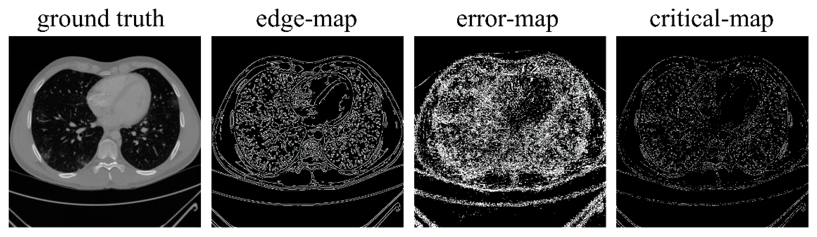
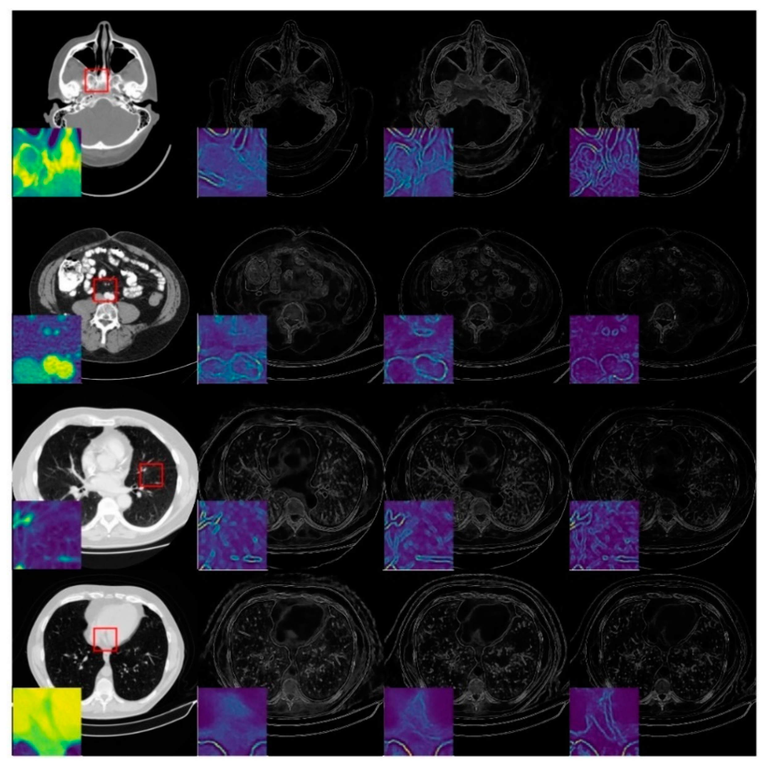
- An image-domain module is proposed to further capture the image space degradation characterization from the frequency-domain reconstruction results. This produces a critical-map to emphasize the contour pixels with high reconstruction errors. The experiments show the favorable achievement of the aid of an image-domain module in the structure preservation and edge enhancement.
2. Materials and Methods
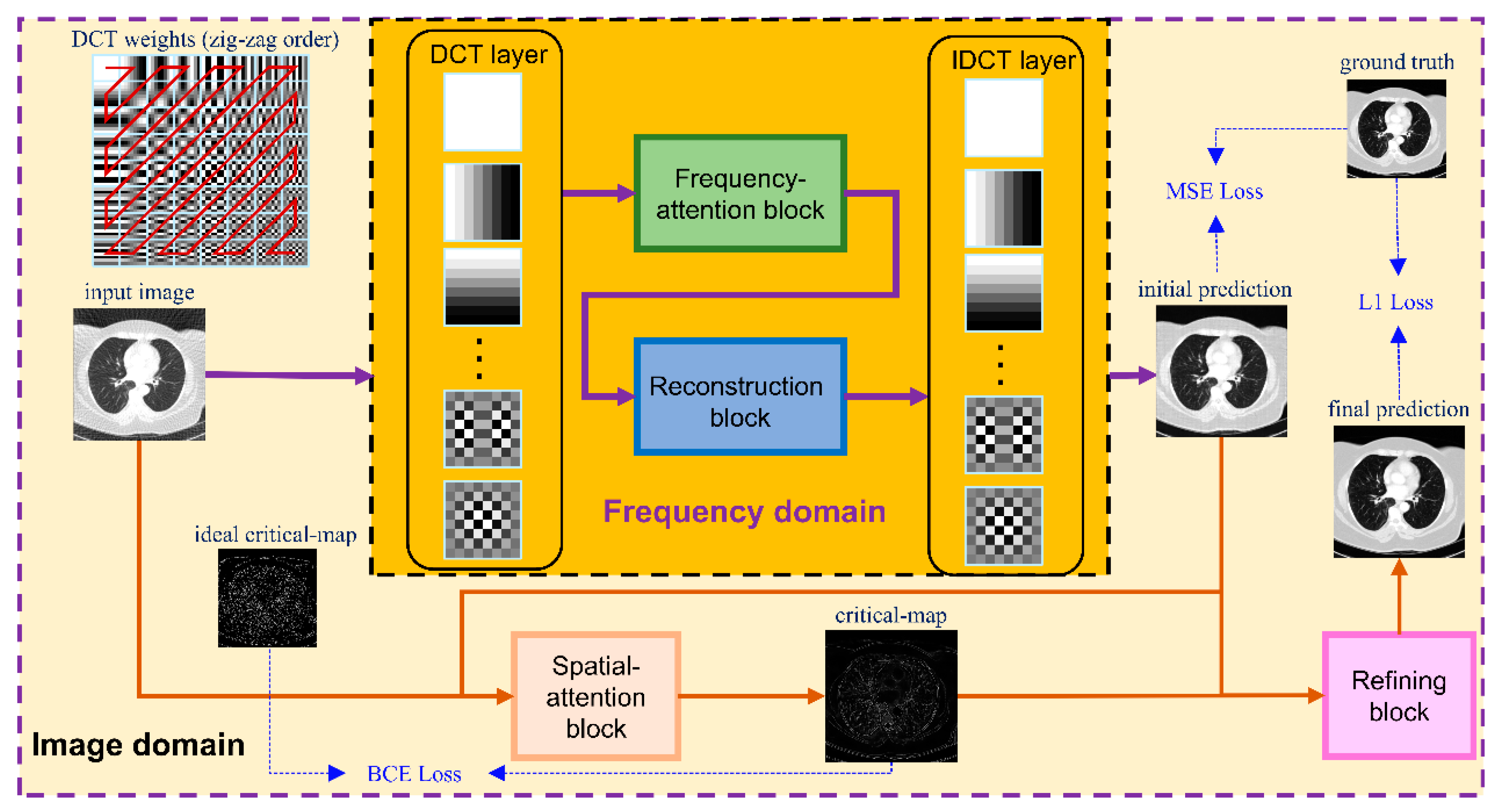
2.1. Network Structure
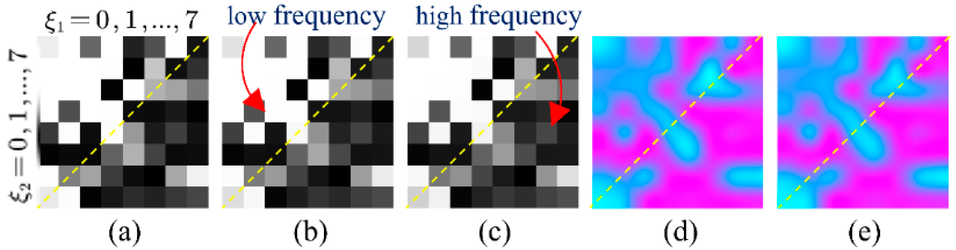
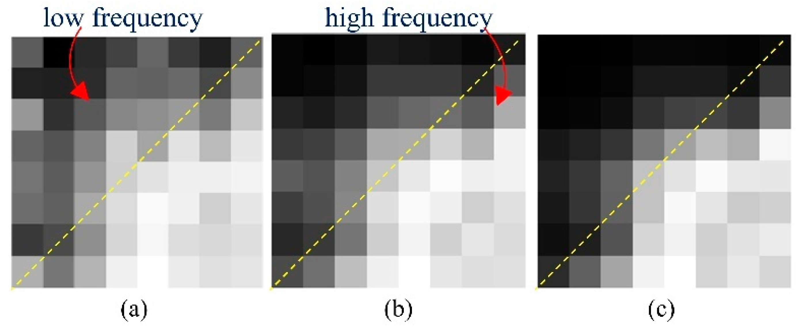
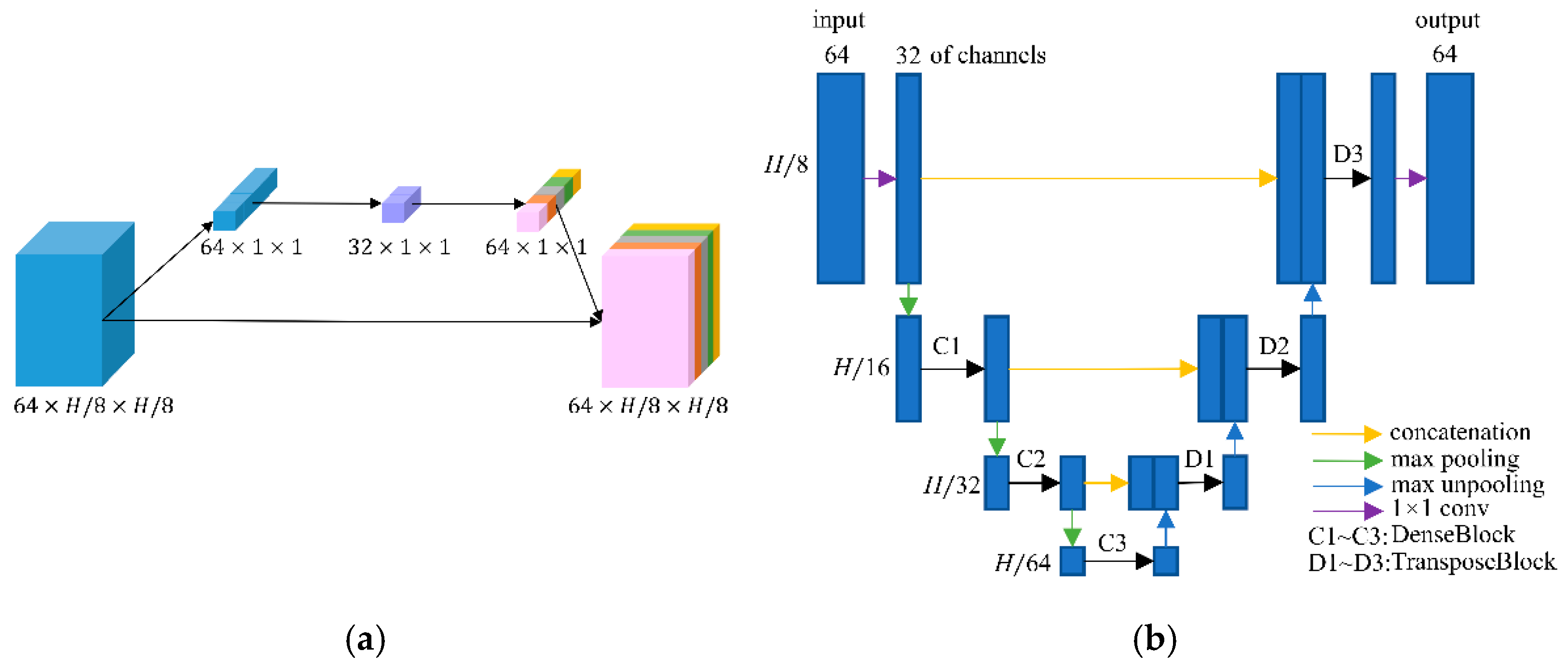
2.2. Frequency-Domain Module
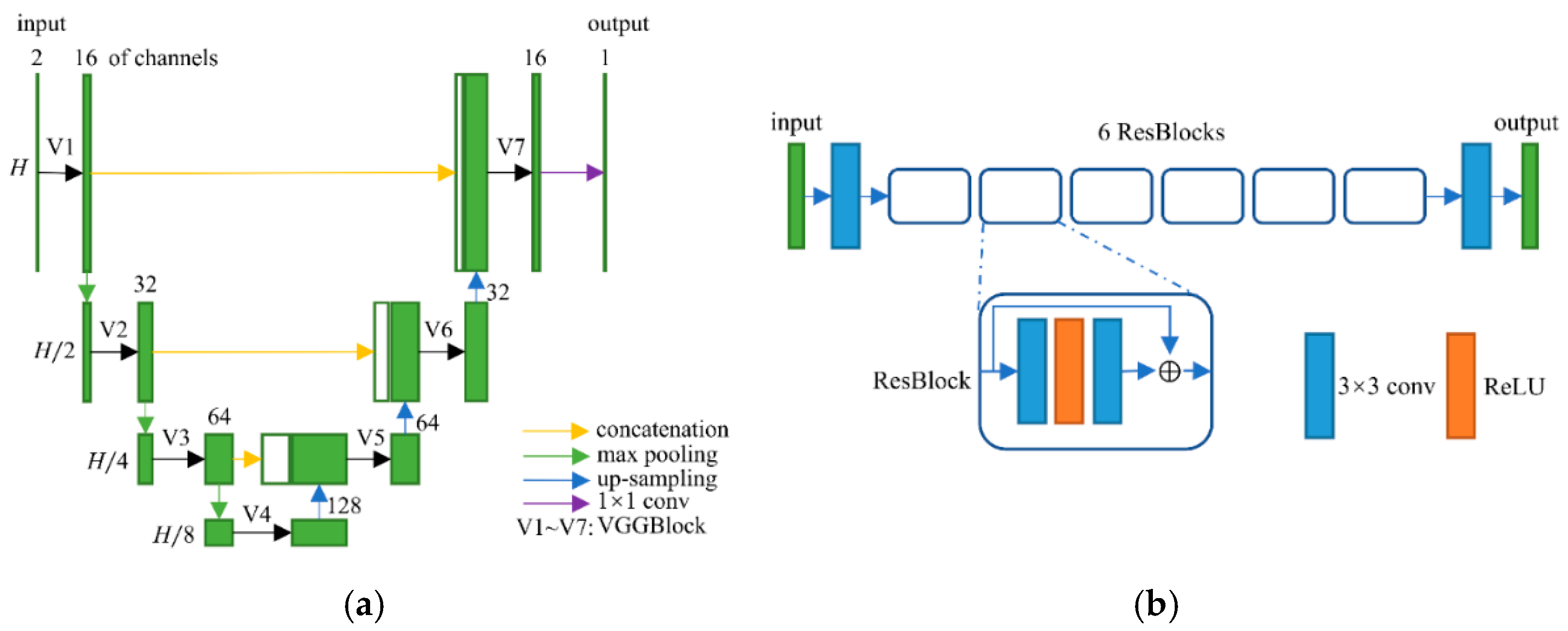
2.3. Image-Domain Module
2.4. Datasets
2.5. Network Training
3. Results
3.1. Degradation-Aware Ability Exploration
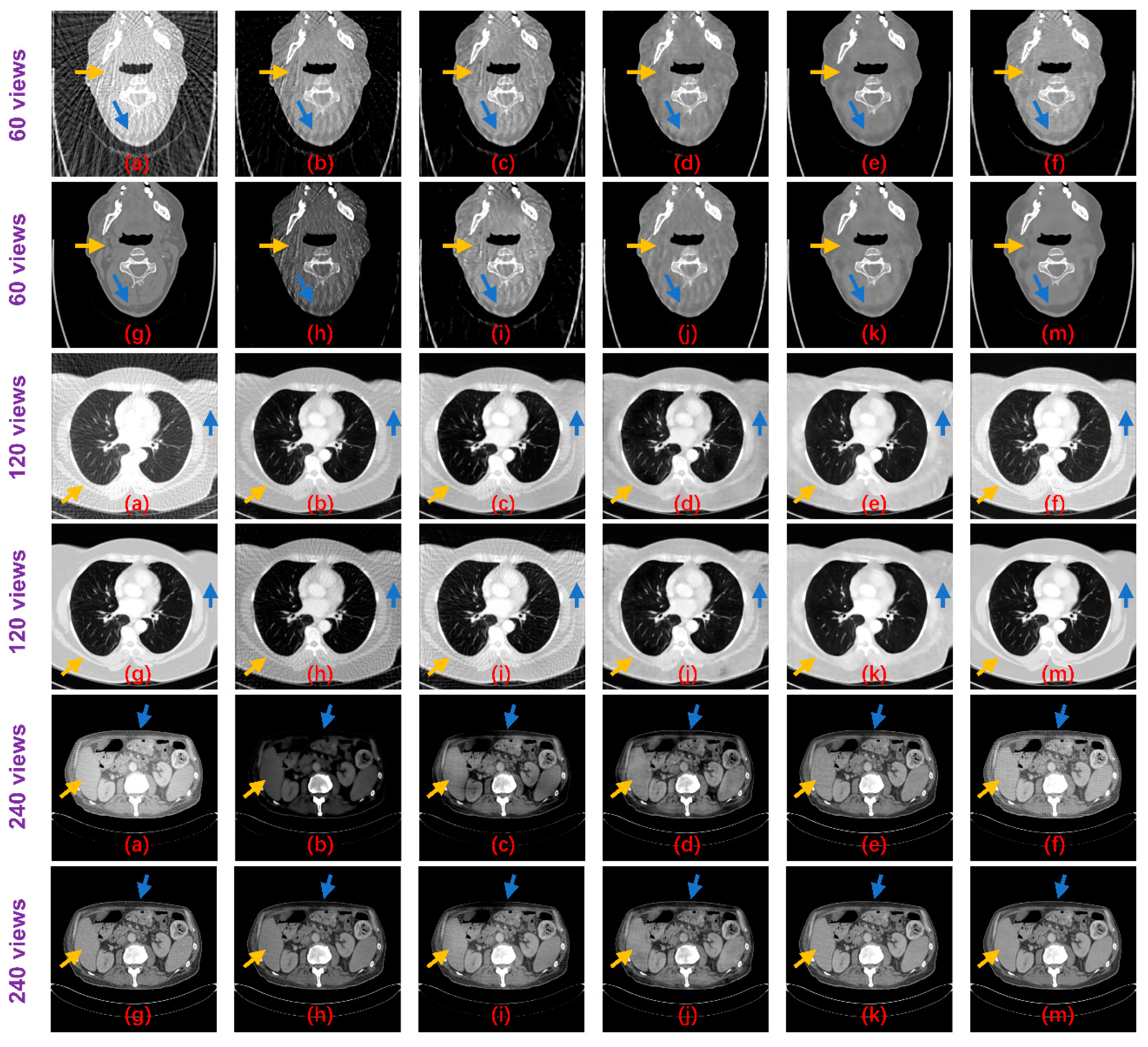
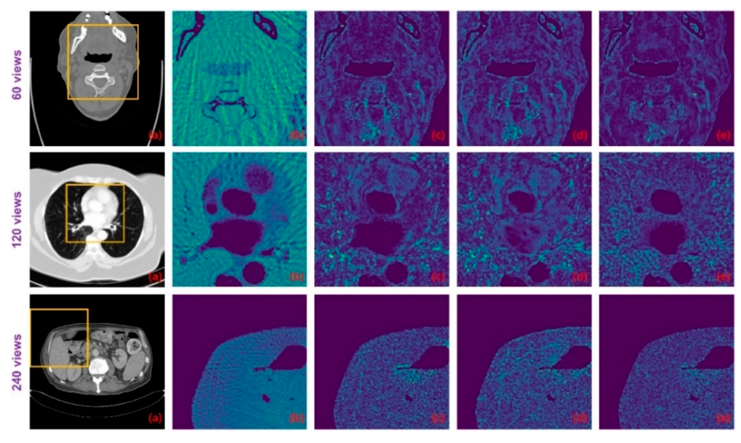
3.2. Reconstruction Performance
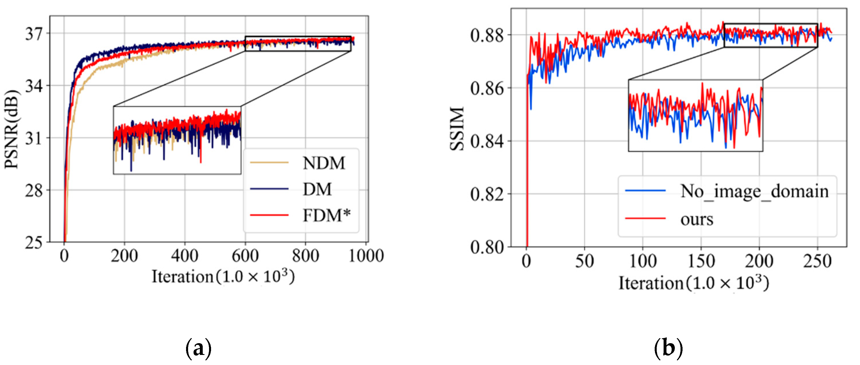
3.3. Ablation Study
3.4. Network Parameter Tuning
4. Discussion
Supplementary Materials
Author Contributions
Funding
Institutional Review Board Statement
Informed Consent Statement
Data Availability Statement
Acknowledgments
Conflicts of Interest
References
- De Chiffre, L.; Carmignato, S.; Kruth, J.P.; Schmitt, R.; Weckenmann, A. Industrial Applications of Computed Tomography. CIRP Annals. 2014, 63, 655–677. [Google Scholar] [CrossRef]
- Brenner, D.J.; Hall, E.J. Computed Tomography—An Increasing Source of Radiation Exposure. N. Engl. J. Med. 2007, 357, 2277–2284. [Google Scholar] [CrossRef] [PubMed] [Green Version]
- Balda, M.; Hornegger, J.; Heismann, B. Ray Contribution Masks for Structure Adaptive Sinogram Filtering. IEEE Trans. Med. Imaging 2012, 31, 1228–1239. [Google Scholar] [CrossRef] [PubMed]
- Manduca, A.; Yu, L.; Trzasko, J.D.; Khaylova, N.; Kofler, J.M.; McCollough, C.M.; Fletcher, J.G. Projection Space Denoising with Bilateral Filtering and CT Noise Modeling for Dose Reduction in CT. Med. Phys. 2009, 36, 4911–4919. [Google Scholar] [CrossRef] [PubMed]
- Boudjelal, A.; Elmoataz, A.; Attallah, B.; Messali, Z. A Novel Iterative MLEM Image Reconstruction Algorithm Based on Beltrami Filter: Application to ECT Images. Tomography 2021, 7, 286–300. [Google Scholar] [CrossRef]
- Aharon, M.; Elad, M.; Bruckstein, A. K-SVD: An Algorithm for Designing Overcomplete Dictionaries for Sparse Representation. IEEE Trans. Signal Process. 2006, 54, 4311–4322. [Google Scholar] [CrossRef]
- Lee, H.; Lee, J.; Cho, S. View-Interpolation of Sparsely Sampled Sinogram Using Convolutional Neural Network. In Medical Imaging 2017: Image Processing, Proceedings of the International Society for Optics and Photonics, Orlando, FL, USA, 12–14 February 2017; SPIE: Bellingham, WA, USA, 2017; Volume 10133, p. 1013328. [Google Scholar]
- Gordon, R.; Bender, R.; Herman, G.T. Algebraic Reconstruction Techniques (Art) for Three-Dimensional Electron Microscopy and X-ray Photography. J. Theor. Biol. 1970, 29, 471–481. [Google Scholar] [CrossRef]
- Andersen, A.H.; Kak, A.C. Simultaneous Algebraic Reconstruction Technique (SART): A Superior Implementation of the ART Algorithm. Ultrason. Imaging 1984, 6, 81–94. [Google Scholar] [CrossRef]
- Trampert, J.; Leveque, J.J. Simultaneous Iterative Reconstruction Technique: Physical Interpretation Based on the Generalized Least Squares Solution. J. Geophys. Res.: Sol. Earth 1990, 95, 12553–12559. [Google Scholar] [CrossRef]
- Candès, E.J.; Romberg, J.; Tao, T. Robust Uncertainty Principles: Exact Signal Reconstruction from Highly Incomplete Frequency Information. IEEE Trans. Inf. Theor. 2006, 52, 489–509. [Google Scholar] [CrossRef] [Green Version]
- Donoho, D.L. Compressed Sensing. IEEE Trans. Inf. Theor. 2006, 52, 1289–1306. [Google Scholar] [CrossRef]
- Sidky, E.Y.; Kao, C.M.; Pan, X. Accurate Image Reconstruction from Few-Views and Limited-Angle Data in Divergent-Beam CT. J. X-Ray Sci. Tech. 2006, 14, 119–139. [Google Scholar]
- Tian, Z.; Jia, X.; Yuan, K.; Pan, T.; Jiang, S.B. Low-Dose Ct Reconstruction via Edge-Preserving Total Variation Regularization. Phys. Med. Biol. 2011, 56, 5949. [Google Scholar] [CrossRef] [PubMed]
- Liu, Y.; Ma, J.; Fan, Y.; Liang, Z. Adaptive-Weighted Total Variation Minimization for Sparse Data Toward Low-Dose X-Ray Computed Tomography Image Reconstruction. Phys. Med. Biol. 2012, 57, 7923. [Google Scholar] [CrossRef]
- Chen, Y.; Gao, D.; Nie, C.; Luo, L.; Chen, W.; Yin, X.; Lin, Y. Bayesian Statistical Reconstruction for Low-Dose X-Ray Computed Tomography Using an Adaptive-Weighting Nonlocal Prior. Comput. Med. Imaging Gr. 2009, 33, 495–500. [Google Scholar] [CrossRef]
- Ma, J.; Zhang, H.; Gao, Y.; Huang, J.; Liang, Z.; Feng, Q.; Chen, W. Iterative Image Reconstruction for Cerebral Perfusion CT Using a Pre-Contrast Scan Induced Edge-Preserving Prior. Phys. Med. Biol. 2012, 57, 7519. [Google Scholar] [CrossRef] [PubMed]
- Zhang, Y.; Xi, Y.; Yang, Q.; Cong, W.; Zhou, J.; Wang, G. Spectral CT Reconstruction with Image Sparsity and Spectral Mean. IEEE Trans. Comput. Imaging. 2016, 2, 510–523. [Google Scholar] [CrossRef] [Green Version]
- Cai, J.F.; Jia, X.; Gao, H.; Jiang, S.; Shen, Z.; Zhao, H. Cine Cone Beam CT Reconstruction Using Low-Rank Matrix Factorization: Algorithm and a Proof-of-Principle Study. IEEE Trans. Med. Imaging 2014, 33, 1581–1591. [Google Scholar] [CrossRef]
- Dabov, K.; Foi, A.; Katkovnik, V.; Egiazarian, K. Image Denoising by Sparse 3-D Transform-Domain Collaborative Filtering. IEEE Trans. Image Process. 2007, 16, 2080–2095. [Google Scholar] [CrossRef]
- Ma, J.; Huang, J.; Feng, Q.; Zhang, H.; Lu, H.; Liang, Z.; Chen, W. Low-Dose Computed Tomography Image Restoration Using Previous Normal-Dose Scan. Med. Phys. 2011, 38, 5713–5731. [Google Scholar] [CrossRef] [Green Version]
- Lauzier, P.T.; Chen, G.H. Characterization of Statistical Prior Image Constrained Compressed Sensing (PICCS): II. Application to Dose Reduction. Med. Phys. 2013, 40, 021902. [Google Scholar] [CrossRef] [Green Version]
- Madesta, F.; Sentker, T.; Gauer, T.; Werner, R. Self-Contained Deep Learning-Based Boosting of 4D Cone-Beam CT Reconstruction. Med. Phys. 2020, 47, 5619–5631. [Google Scholar] [CrossRef]
- Zhang, Z.; Liang, X.; Dong, X.; Xie, Y.; Cao, G. A Sparse-View CT Reconstruction Method Based on Combination of DenseNet and Deconvolution. IEEE Trans. Med. Imaging 2018, 37, 1407–1417. [Google Scholar] [CrossRef]
- Chen, H.; Zhang, Y.; Kalra, M.K.; Lin, F.; Chen, Y.; Liao, P.; Zhou, J.; Wang, G. Low-Dose CT with a Residual Encoder-Decoder Convolutional Neural Network. IEEE Trans. Med. Imaging 2017, 36, 2524–2535. [Google Scholar] [CrossRef]
- Ronneberger, O.; Fischer, P.; Brox, T. U-Net: Convolutional Networks for Biomedical Image Segmentation. In Proceedings of the International Conference on Medical Image Computing and Computer-Assisted Intervention, Munich, Germany, 5–9 October 2015; Volume 1, pp. 234–241. [Google Scholar]
- Han, Y.; Ye, J.C. Framing U-Net via Deep Convolutional Framelets: Application to Sparse-View CT. IEEE Trans. Med. Imaging 2018, 37, 1418–1429. [Google Scholar] [CrossRef] [Green Version]
- Xie, S.; Zheng, X.; Chen, Y.; Xie, L.; Liu, J.; Zhang, Y.; Yan, J.; Zhu, H.; Hu, Y. Artifact Removal Using Improved GoogLeNet for Sparse-View CT Reconstruction. Sci. Rep. 2018, 8, 1–9. [Google Scholar]
- Clark, K.; Vendt, B.; Smith, K.; Freymann, J.; Kirby, J.; Koppel, P.; Moore, S.; Phillips, S.; Maffitt, D.; Pringle, M.; et al. The Cancer Imaging Archive (TCIA): Maintaining and operating a public information repository. J. Digit. Imaging 2013, 26, 1045–1057. [Google Scholar] [CrossRef] [PubMed] [Green Version]
- Roth, H.; Lu, L.; Seff, A.; Cherry, K.M.; Hoffman, J.; Wang, S.; Liu, J.; Turkbey, E.; Summers, R.M. A New 2.5 D Representation for Lymph Node Detection in CT [Dataset]. The Cancer Imaging Archive. Available online: https://wiki.cancerimagingarchive.net/display/Public/CT+Lymph+Nodes (accessed on 8 April 2021). [CrossRef]
- Wu, H.; Huang, J. Secure JPEG Steganography by LSB+ Matching and Multi-Band Embedding. In Proceedings of the 18th IEEE International Conference on Image Processing (ICIP 2011), Brussels, Belgium, 11–14 September 2011; Volume 1, pp. 2737–2740. [Google Scholar]
- Hu, J.; Shen, L.; Sun, G. Squeeze-and-Excitation Networks. In Proceedings of the IEEE Conference on Computer Vision and Pattern Recognition (CVPR 2018), Salt Lake City, UT, USA, 18–22 June 2018; Volume 1, pp. 7132–7141. [Google Scholar]
- Zhang, X.; Wu, X. Attention-Guided Image Compression by Deep Reconstruction of Compressive Sensed Saliency Skeleton. In Proceedings of the IEEE Conference on Computer Vision and Pattern Recognition (CVPR 2018), Salt Lake City, UT, USA, 18–22 June 2018; Volume 1, pp. 13354–13364. [Google Scholar]
- Kinahan, P.; Muzi, M.; Bialecki, B.; Coombs, L. Data from ACRIN-FMISO-Brain [Dataset]. The Cancer Imaging Archive. Available online: https://wiki.cancerimagingarchive.net/pages/viewpage.action?pageId=33948305 (accessed on 18 February 2021). [CrossRef]
- National Cancer Institute Clinical Proteomic Tumor Analysis Consortium (CPTAC). (2018). Radiology Data from the Clinical Proteomic Tumor Analysis Consortium Head and Neck Squamous Cell Carcinoma [CPTAC-HNSCC] Collection [Dataset]. The Cancer Imaging Archive. Available online: https://wiki.cancerimagingarchive.net/display/Public/CPTAC-HNSCC (accessed on 3 November 2021). [CrossRef]
- Lucchesi, F.R.; Aredes, N.D. Radiology Data from The Cancer Genome Atlas Esophageal Carcinoma [TCGA-ESCA] Collection [Dataset]. The Cancer Imaging Archive. Available online: https://wiki.cancerimagingarchive.net/display/Public/TCGA-ESCA (accessed on 3 June 2020). [CrossRef]
- Wang, J.; Li, T.; Lu, H.; Liang, Z. Penalized Weighted Least-Squares Approach to Sinogram Noise Reduction and Image Reconstruction for Low-Dose X-Ray Computed Tomography. IEEE Trans. Med. Imaging. 2006, 25, 1272–1283. [Google Scholar] [CrossRef] [PubMed]
- Defrise, M.; Vanhove, C.; Liu, X. An Algorithm for Total Variation Regularization in High-Dimensional Linear Problems. Inverse Probl. 2011, 27, 065002. [Google Scholar] [CrossRef]
- Lasio, G.M.; Whiting, B.R.; Williamson, J.F. Statistical Reconstruction for X-Ray Computed Tomography Using Energy-Integrating Detectors. Phys. Med. Biol. 2007, 52, 2247. [Google Scholar] [CrossRef]
- Adler, J.; Kohr, H.; Oktem, O. Operator Discretization Library (ODL). Software. Available online: https://github.com/odlgroup/odl (accessed on 2 September 2016).
- Hui, Z.; Wang, X.; Gao, X. Fast and Accurate Single Image Super-Resolution via Information Distillation Network. In Proceedings of the IEEE Conference on Computer Vision and Pattern Recognition, 2018 (CVPR 2018), Salt Lake City, UT, USA, 18–22 June 2018; Volume 1, pp. 723–731. [Google Scholar]
- Lim, B.; Son, S.; Kim, H.; Nah, S.; Lee, K.M. Enhanced Deep Residual Networks for Single Image Super-Resolution. In Proceedings of the IEEE Conference on Computer Vision and Pattern Recognition Workshops, Honolulu, HI, USA, 21–26 July 2017; (CVPR Workshops, 2017). Volume 1, pp. 136–144. [Google Scholar]
- Paszke, A.; Gross, S.; Chintala, S.; Chanan, G.; Yang, E.; DeVito, Z.; Lin, Z.; Desmaison, A.; Antiga, L.; Lerer, A. Automatic Differentiation in PyTorch. In Proceedings of the International Conference on Neural Information Processing Systems Workshop: The Future of Gradient-based Machine Learning Software and Techniques, Long Beach, CA, USA, 4–9 December 2017. [Google Scholar]
- Kingma, D.P.; Ba, J. Adam: A Method for Stochastic Optimization. arXiv 2014, arXiv:1412.6980. [Google Scholar]
- Walpole, R.E.; Myers, R.H.; Myers, S.L.; Ye, K.E. Probability and Statistics for Engineers and Scientists, 7th ed.; Pearson: New Delhi, India, 2006. [Google Scholar]


| Method | Number of Parameters | Computational Cost (per Image) |
|---|---|---|
| Improved GoogLeNet | 1.25 M | 0.0032 s |
| Tight frame U-Net | 31.42 M | 0.0034 s |
| RED-CNN | 1.85 M | 0.0010 s |
| DD-Net | 0.56 M | 0.0057 s |
| FDM | 0.92 M | 0.0050 s |
| Improved GoogLeNet+ | 3.75 M | 0.0032 s |
| Tight frame U-Net+ | 94.26 M | 0.0034 s |
| RED-CNN+ | 5.55 M | 0.0010 s |
| DD-Net+ | 1.68 M | 0.0057 s |
| ours | 1.63 M | 0.0062 s |
| Views | Body Part | FBP | Improved GoogLeNet | Tight Frame U-Net | RED-CNN | DD-Net | FDM |
|---|---|---|---|---|---|---|---|
| 60 | Head | 15.9478/0.3516 | 21.6936/0.4607 | 25.0216/0.6051 | 31.0674/0.8171 | 35.4189/0.9147 | 33.8139/0.8088 |
| Abdomen | 14.6239/0.3977 | 19.5052/0.4886 | 25.3207/0.6907 | 32.2187/0.8760 | 35.9957/0.9237 | 35.8076/0.9028 | |
| Lung | 15.7114/0.4177 | 21.1298/0.5315 | 25.1913/0.6981 | 30.2601/0.8481 | 33.9357/0.9080 | 33.4616/0.8532 | |
| Esophagus | 13.8681/0.3428 | 18.2902/0.4173 | 24.0947/0.6291 | 31.9415/0.8446 | 35.6552/0.9220 | 34.8013/0.8327 | |
| 120 | Head | 20.5276/0.4536 | 32.3011/0.7400 | 34.5627/0.8666 | 34.5000/0.8859 | 39.4975/0.9488 | 36.5722/0.8386 |
| Abdomen | 18.6596/0.4940 | 29.1715/0.7059 | 33.0186/0.9035 | 35.2896/0.9210 | 39.3417/0.9496 | 38.4492/0.9184 | |
| Lung | 20.0424/0.5333 | 29.9168/0.7671 | 31.6234/0.8894 | 33.0130/0.8990 | 37.0283/0.9388 | 36.7272/0.8877 | |
| Esophagus | 17.2796/0.4285 | 27.0452/0.6057 | 32.2867/0.8630 | 34.7532/0.8904 | 38.8522/0.9518 | 37.1417/0.8544 | |
| 240 | Head | 26.5085/0.5865 | 32.4706/0.8255 | 36.7117/0.9150 | 37.1478/0.9052 | 42.6465/0.9660 | 38.4318/0.8443 |
| Abdomen | 25.4890/0.6368 | 31.2142/0.8480 | 34.9420/0.9465 | 36.7007/0.9384 | 41.8674/0.9654 | 41.0545/0.9425 | |
| Lung | 25.6982/0.6791 | 29.5797/0.8113 | 33.2487/0.9263 | 35.1415/0.9260 | 39.1089/0.9560 | 38.6735/0.9058 | |
| Esophagus | 23.0284/0.5516 | 34.1418/0.8526 | 34.6916/0.9156 | 37.3571/0.9097 | 41.3469/0.9687 | 39.7422/0.8852 | |
| Views | Body Part | SART | Improved GoogLeNet+ | Tight Frame U-Net+ | RED-CNN+ | DD-Net+ | Ours |
| 60 | Head | 23.4269/0.6964 | 28.0190/0.7486 | 25.8151/0.6176 | 31.4201/0.8158 | 35.5668/0.9256 | 36.0998/0.9421 |
| Abdomen | 18.4496/0.6381 | 28.3975/0.7401 | 25.3411/0.6758 | 32.1736/0.8687 | 36.0104/0.9338 | 36.8327/0.9434 | |
| Lung | 17.1589/0.6097 | 27.2493/0.7354 | 25.6127/0.6899 | 30.1739/0.8490 | 33.7070/0.9152 | 34.9458/0.9291 | |
| Esophagus | 18.5389/0.6526 | 29.2958/0.7119 | 24.2923/0.6177 | 31.7161/0.8389 | 35.1918/0.9291 | 36.4700/0.9428 | |
| 120 | Head | 28.6282/0.7748 | 30.8313/0.7143 | 30.0908/0.6645 | 35.4605/0.8824 | 39.5932/0.9517 | 40.2681/0.9630 |
| Abdomen | 23.1838/0.7338 | 28.2309/0.6705 | 27.7061/0.6966 | 35.7323/0.9180 | 39.4556/0.9521 | 40.1679/0.9606 | |
| Lung | 21.6494/0.7158 | 27.6462/0.6789 | 28.7425/0.7372 | 33.3552/0.9009 | 37.1235/0.9433 | 38.3021/0.9525 | |
| Esophagus | 22.7435/0.7335 | 26.2278/0.5736 | 25.9611/0.6196 | 35.0883/0.8977 | 39.0283/0.9550 | 39.5306/0.9625 | |
| 240 | Head | 34.5998/0.8424 | 35.8046/0.8199 | 34.5272/0.7890 | 38.4972/0.9242 | 43.3962/0.9727 | 43.8769/0.9755 |
| Abdomen | 29.7504/0.8250 | 35.0612/0.8505 | 32.7387/0.8281 | 37.7709/0.9488 | 42.3253/0.9712 | 43.0279/0.9724 | |
| Lung | 27.7240/0.8141 | 33.6383/0.8704 | 31.9236/0.8353 | 35.7299/0.9385 | 39.9550/0.9641 | 40.7020/0.9670 | |
| Esophagus | 28.4788/0.8112 | 32.4359/0.7369 | 30.5312/0.7478 | 37.2861/0.9355 | 41.8500/0.9743 | 42.2515/0.9745 |
| Metric | Views | Standard Deviation | Confidence Interval |
|---|---|---|---|
| PSNR | 60 | 3.0346 | (35.8188 ± 0.1883) |
| 120 | 3.2308 | (39.2702 ± 0.2005) | |
| 240 | 3.5828 | (42.0365 ± 0.2223) | |
| SSIM | 60 | 0.0214 | (0.9368 ± 0.0013) |
| 120 | 0.0181 | (0.9577 ± 0.0011) | |
| 240 | 0.0164 | (0.9708 ± 0.0010) |
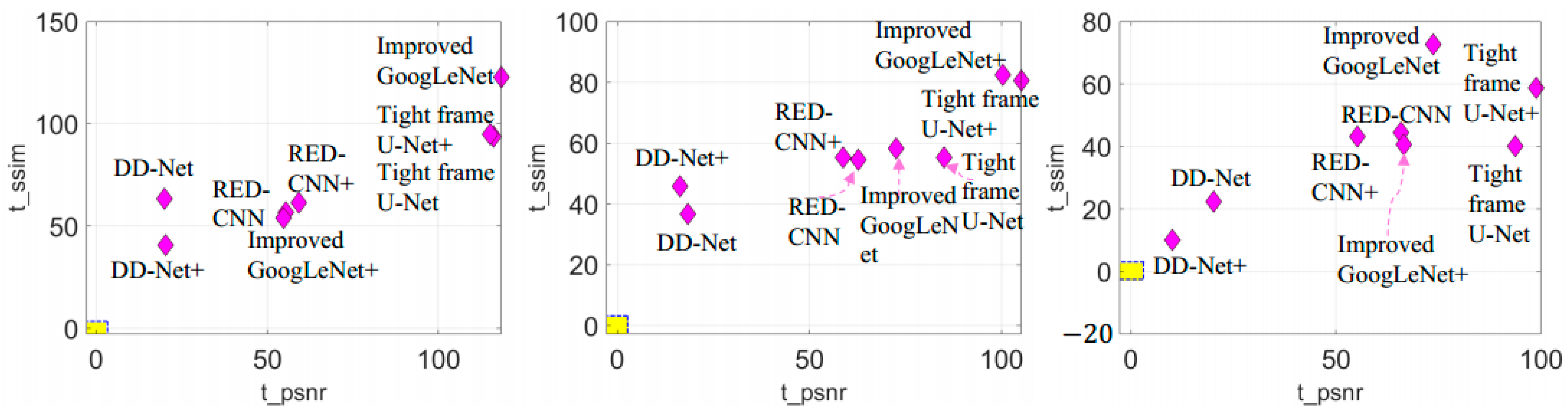
| Compared Method | 60 Views | 120 Views | 240 Views | |||
|---|---|---|---|---|---|---|
| t_psnr | t_ssim | t_psnr | t_ssim | t_psnr | t_ssim | |
| Improved GoogLeNet | 118.2965 | 122.8433 | 72.5626 | 58.2919 | 73.6602 | 72.7600 |
| Tight frame U-Net | 116.1232 | 93.8206 | 85.0838 | 55.3261 | 93.7110 | 40.0548 |
| RED-CNN | 55.4372 | 56.7843 | 62.7069 | 54.5588 | 65.8841 | 44.3951 |
| DD-Net | 19.9694 | 63.3336 | 18.4503 | 36.6697 | 20.1678 | 22.4695 |
| Improved GoogLeNet+ | 54.7750 | 54.1022 | 100.2554 | 82.4739 | 66.5465 | 40.6918 |
| Tight frame U-Net+ | 115.1382 | 94.8125 | 105.0866 | 80.6470 | 98.7682 | 58.7093 |
| RED-CNN+ | 59.2286 | 61.5391 | 58.8350 | 55.3430 | 55.2423 | 43.2324 |
| DD-Net+ | 20.3308 | 40.7363 | 16.3571 | 45.8754 | 10.0287 | 10.1868 |
| Views | Body Part | NDM | DM | FDM* |
|---|---|---|---|---|
| 60 | Head | 32.8563 | 32.5425 | 33.7495 |
| Abdomen | 32.8446 | 32.6188 | 35.6840 | |
| Lung | 32.9257 | 32.6978 | 33.1673 | |
| Esophagus | 32.8197 | 32.6037 | 33.7173 | |
| 120 | Head | 35.7321 | 35.5704 | 36.5904 |
| Abdomen | 35.8170 | 35.6162 | 38.1990 | |
| Lung | 35.6267 | 35.5710 | 36.1079 | |
| Esophagus | 35.7173 | 35.5953 | 36.1940 | |
| 240 | Head | 37.6943 | 37.5759 | 38.4270 |
| Abdomen | 37.9056 | 37.6344 | 40.3256 | |
| Lung | 37.6960 | 37.4694 | 38.2643 | |
| Esophagus | 37.6851 | 37.3774 | 38.1505 |
| Views | Body Part | No_Image_Domain | Ours |
| 60 | Head | 0.9396 | 0.9421 |
| Abdomen | 0.9415 | 0.9434 | |
| Lung | 0.9268 | 0.9291 | |
| Esophagus | 0.9404 | 0.9428 | |
| 120 | Head | 0.9619 | 0.9630 |
| Abdomen | 0.9596 | 0.9606 | |
| Lung | 0.9510 | 0.9525 | |
| Esophagus | 0.9612 | 0.9625 | |
| 240 | Head | 0.9751 | 0.9755 |
| Abdomen | 0.9719 | 0.9724 | |
| Lung | 0.9660 | 0.9670 | |
| Esophagus | 0.9739 | 0.9745 |
Publisher’s Note: MDPI stays neutral with regard to jurisdictional claims in published maps and institutional affiliations. |
© 2021 by the authors. Licensee MDPI, Basel, Switzerland. This article is an open access article distributed under the terms and conditions of the Creative Commons Attribution (CC BY) license (https://creativecommons.org/licenses/by/4.0/).
Share and Cite
Sun, C.; Liu, Y.; Yang, H. Degradation-Aware Deep Learning Framework for Sparse-View CT Reconstruction. Tomography 2021, 7, 932-949. https://doi.org/10.3390/tomography7040077
Sun C, Liu Y, Yang H. Degradation-Aware Deep Learning Framework for Sparse-View CT Reconstruction. Tomography. 2021; 7(4):932-949. https://doi.org/10.3390/tomography7040077
Chicago/Turabian StyleSun, Chang, Yitong Liu, and Hongwen Yang. 2021. "Degradation-Aware Deep Learning Framework for Sparse-View CT Reconstruction" Tomography 7, no. 4: 932-949. https://doi.org/10.3390/tomography7040077
APA StyleSun, C., Liu, Y., & Yang, H. (2021). Degradation-Aware Deep Learning Framework for Sparse-View CT Reconstruction. Tomography, 7(4), 932-949. https://doi.org/10.3390/tomography7040077