3.1.1. Theory
This work achieves significant generalization of the geometric-optical tomography theory developed in [
13,
14], extending it to weak inhomogeneities in absorbing media. We have also developed an appropriate tomography algorithm based on this theory. As in [
14], the theory starting point is the Radon transform for the measurement geometry under consideration.
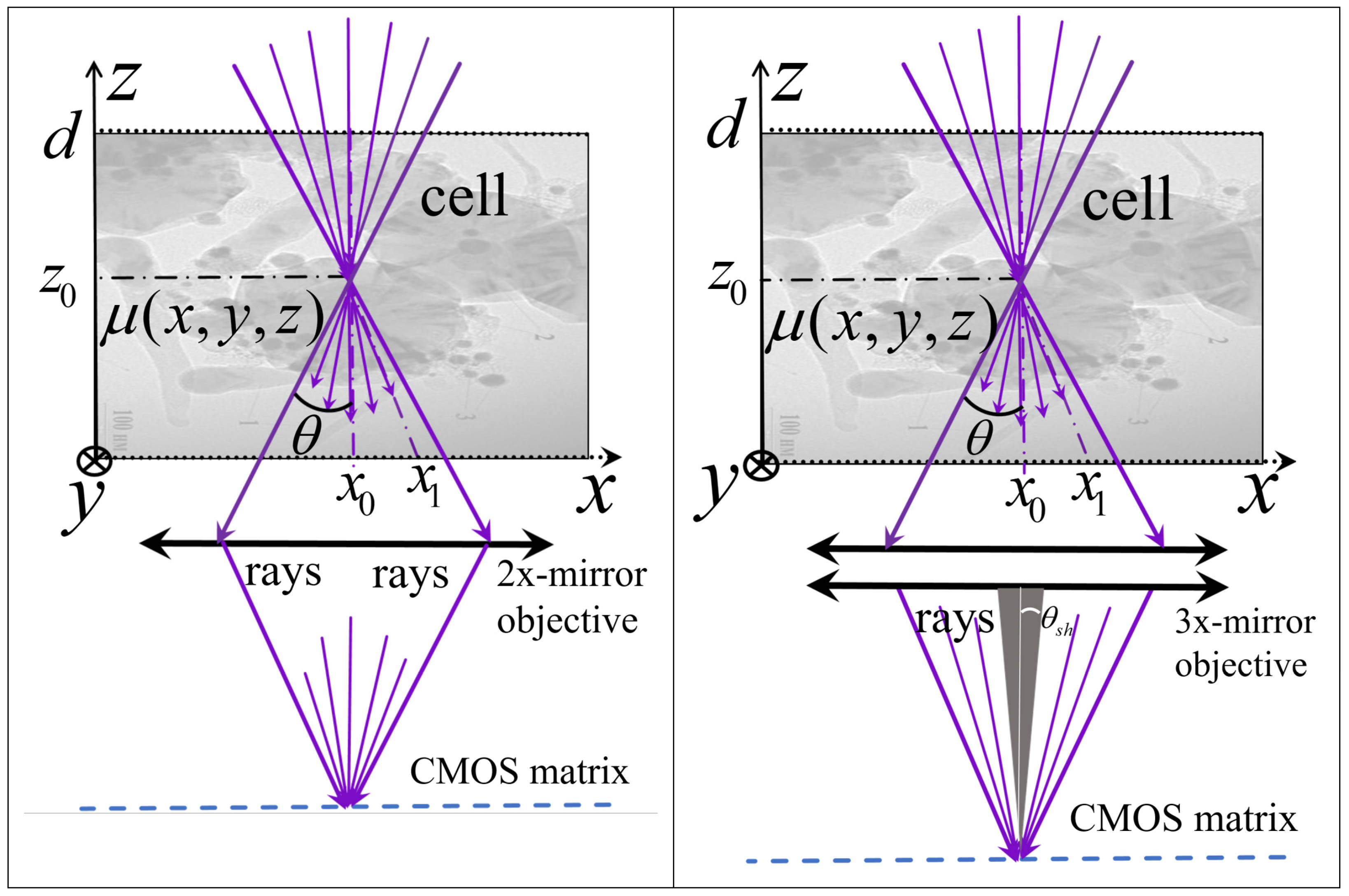
The analysis is based on the radiation transport equation in an absorbing medium, where the intensity at the absorbing layer exit is determined by optical depth
, which is the integral of the absorption coefficient along the beam path on a straight line passing through points
x0,
y0,
z0 and
x1,
y1,
z1 = 0 between planes
z = 0 and
z =
d (see in
Figure 2):
Using the integral parametric representation in (1) and integrating over all rays within the cone exiting through the
z = 0 plane, we can obtain the direct problem solution, which is the signal intensity ratio with and without the analyzed object
at the corresponding point of the CMOS matrix (Radon transformation in the measurement geometry under consideration) [
13]:
The most well known methods of medical tomography, CT (X-ray computed tomography) and MRI (magnetic resonance imaging), also lead to similar but different Radon transformations because, unlike axial tomography considered here, these methods use circular scanning. These methods are based on solving corresponding inverse problems in cylindrical coordinates, which creates specific challenges when transforming to images in Cartesian coordinates. Their theory was first developed by Radon [
16] and later applied in computed X-ray tomography by A.N. Tikhonov [
17], in line with his theory of incorrect inverse problems.
Unlike CT and MRI, the initial equation in this problem is nonlinear, creating serious theoretical and computational challenges. In the solution method [
13,
14], the problem was solved in the small optical absorption thickness approximation
τ << 1, enabling exponential decomposition and obtaining a linear 3D convolution-type integral equation for the desired distribution
μ(
x,
y,
z). In this approximation, for relative intensity decrease, we obtain the expression [
13,
14]:
After transformations and integration over variables
x1,
y1, a 3D convolution tomography equation is obtained [
13,
14]:
where the conditions for finding radiation within the cone are also included in the kernel of the equation
K. Three-dimensional Fourier transform of (4) yields a simple
k-space spectrum equation:
and the Radon inverse transformation formula for this tomography method:
where Fourier transforms use the same notation as transformed parameters, differing only in arguments.
This enabled algorithm development is based on inverse Fourier transform [
13]. During algorithm development, we had to address the problem of kernel divergence in Equation
K (5) at the focal point. In [
13], the value of
K at the focal point was chosen by extrapolation from neighboring pixels, and the algorithm was tested in numerical simulations on a 20 × 20 × 20 grid. Due to small dimensionality, test inhomogeneities exhibited noticeable blurring. Significant discretization errors led to the amplification of simulated random errors, i.e., the manifestation of ill-posedness, which required the application of Tikhonov regularization.
In our subsequent paper [
14], the algorithm was refined for application to plant-cell analysis using data from measurements with the ×46 microscope. Measurements were performed with 256 × 256 × 219 discretization at a pixel size of 140 nm, chosen based on the scale of diffraction-related beam blurring. It turned out that the choice of kernel value at the focal pixel made in [
13] was impractical. Varying this parameter allowed us to determine its optimal value by maximizing the observed resolution of the smallest details in reconstructions of the studied objects. As a result, 140 nm resolution of observed organelles was achieved in reconstructions of relatively transparent cell regions.
Numerical simulations showed that the algorithm does not exhibit properties of an ill-posed problem—it does not amplify added random errors and accurately reproduces test objects without added errors. Apparently, this property is due to the presence of a weak singularity in the kernel of the equation being solved—such problems, like the inverse Abel transform, which has an exact solution, can possess this feature. Therefore, regularization was not applied in the cell analysis presented in [
14]. This specificity of axial tomography is an important advantage compared to standard CT.
Unfortunately, the conditions of low absorption were not satisfied in most of the volume of the studied cells, which limited the accuracy of the determined absorption coefficient of the observed inhomogeneities.
This paper obtains significant theory generalization for weak inhomogeneities in absorbing media and develops an appropriate tomography algorithm. The tomography-integral equation is derived from Formula (1), which describes radiation intensity in the geometric-optical approximation, assuming absorption coefficient inhomogeneity is small compared to the constant absorption component in the analyzed region
:
By performing transformations and substitutions of variables, similar to those described in [
13], and including the limits of integration in the kernel of the equation, we obtain a 3D convolution-type integral tomography equation with a weak singularity kernel. This equation can be expressed explicitly as:
where
is the measured signal intensity distribution ratio to signal without object depending on focus position, and
is a theoretical correction accounting for the medium constant absorption component, explicitly represented by the first term on Equation (8), right-hand side:
where
d is the vertical size of the analysis area and
is the angle between the ray cone generatrix and the vertical axis. This simple formula has independent interest, as it determines the signal from a layer with a constant absorption coefficient, enabling inverse problem solution: determining the homogeneous layer absorption coefficient from the measured signal. This has obvious practical significance and can be used for calibration in our proposed tomography method.
Comparing kernel functions in (5) and (10), in (10), a multiplier accounting for the constant absorption component has appeared. At = 0, these formulas coincide.
Three-dimensional Fourier transform of Equation (9) leads to a
k-space spectrum equation similar to (6):
and its Cartesian coordinate solution is expressed as:
Generally, solving inverse problems such as convolution using input data containing errors can be ill-posed. Random errors can have broader spatial spectra than the kernel, leading to uncontrolled small-scale feature amplification in solutions. To address this, Tikhonov regularization [
17] can be applied when necessary.
In the proposed method (9)–(13), in which the kernel K in (10) has the same divergence as the above-considered kernel in (5), more accurate scaling is achieved by using the ratio (11) between the signal from vertically homogeneous layers of the objects under study and their absorption coefficient.
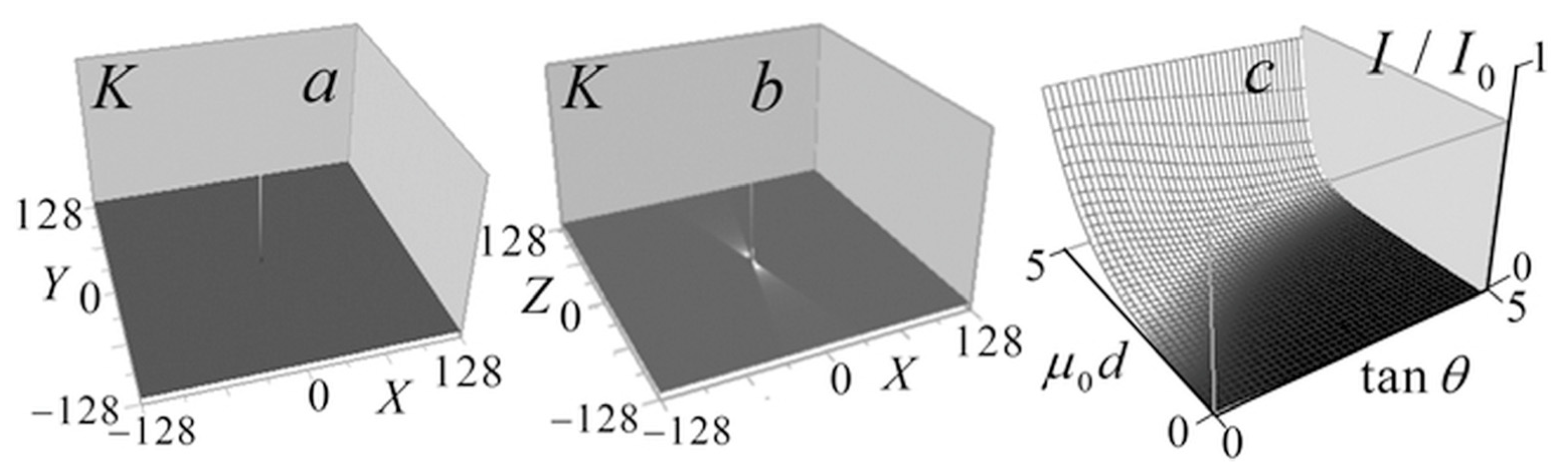
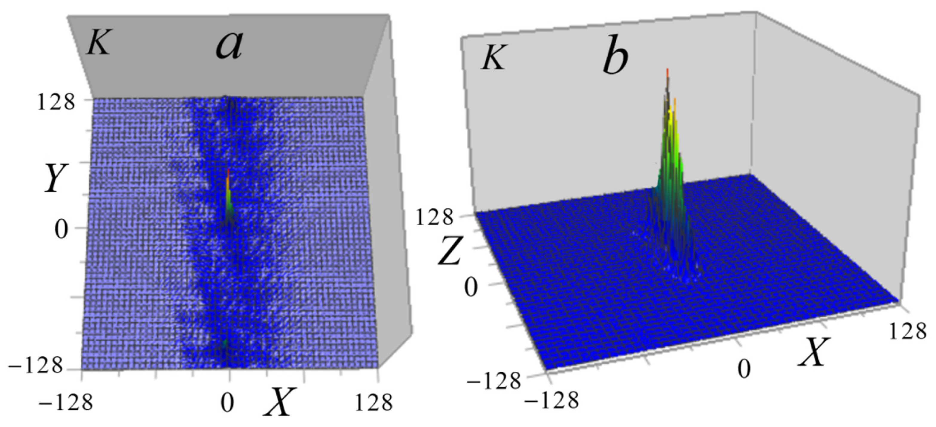
Figure 3 shows the kernel
K (10) of the tomography Equation (9), and the distribution of the correction term (11) in the left-hand side of this equation, depending on the arguments
.
Unlike the kernel in the low-absorption approximation [
13,
14], in this case, this kernel distribution is not universal but depends on the analyzed object absorption coefficient constant component
. The kernel peak (
Figure 3a) manifests as a discrete
δ-function, forming a pedestal in its spatial spectrum, ensuring method resolution down to the smallest scales determined by signal blurring in focus. The correction term distribution in
Figure 3c shows a decrease with increasing absorption and light-cone angle
. The one-to–one correspondence between
and the argument
for any angle
enables considering this distribution as an inverse problem solution for determining
, i.e., as a method for determining the homogeneous layer absorption coefficient of
from the measured signal attenuation
.
This result is important not only as a method for determining the absorption coefficient of homogeneous layers, but also as a calibration method for 3D reconstructions in axial tomography. If a quasi-homogeneous layer () can be identified in the analyzed object, we determine its absorption coefficient and choose the focal kernel value in (10) such that the absorption of this layer in the reconstruction corresponds to . This value, together with the value of the constant component of the absorption distribution, determines the scale for calibrating the reconstruction (13). If necessary, an artificial layer with a known absorption coefficient can be placed together with the object.
3.1.2. Numerical Simulation
When developing algorithms based on solving inverse problems described by integral equations, solution accuracy is not directly proportional to the error level and depends on the specifics of the structure of a particular analyzed object. Additionally, artifacts may arise during reconstruction. Therefore, numerical simulation plays a crucial role as a necessary research stage.
For the tomography algorithms (6)–(10), numerical simulations were performed for test objects with given geometric structure (point-like, homogeneous in absorption coefficient, and heterogeneous modeled by Gaussian distributions). The study was conducted using a closed loop: (a) for each focus position, the 3D received signal distribution is calculated; (b) a random Gaussian “measurement error” with zero mean and a specified standard deviation is added to the signal; (c) the inverse problem (9–10) is solved; (d) the resulting solution is compared with the initial distribution.
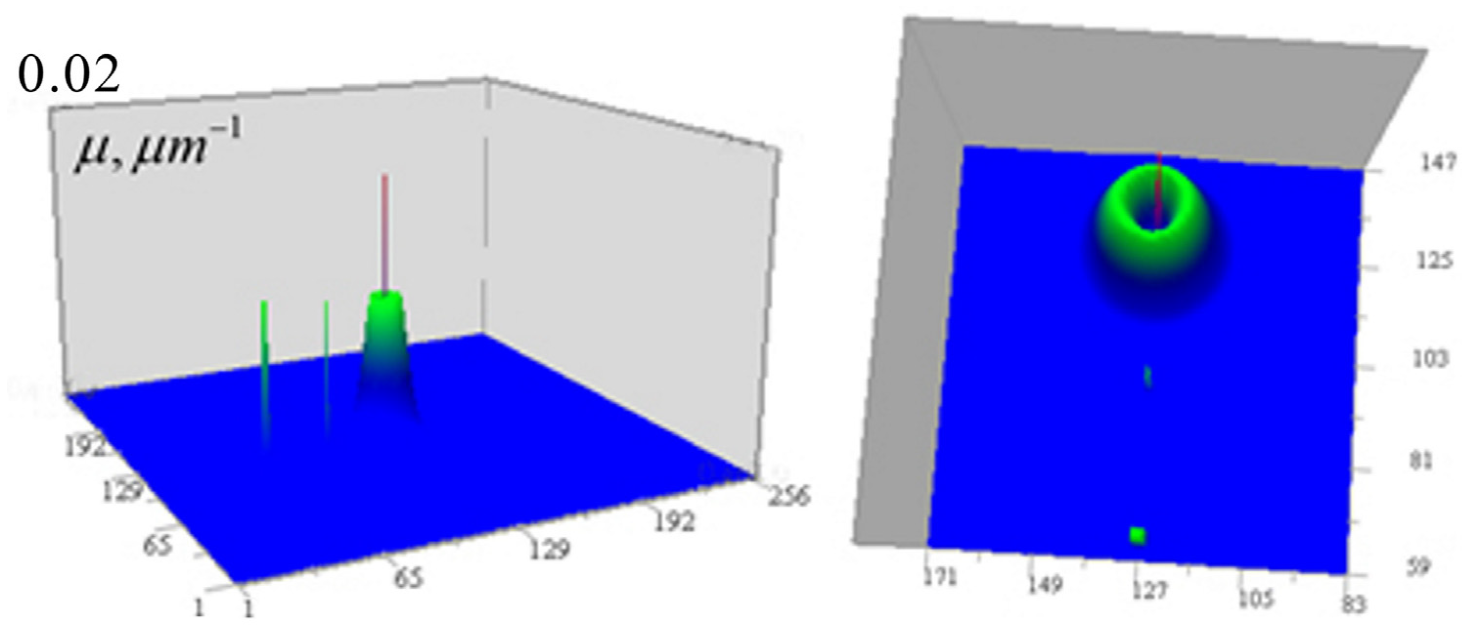
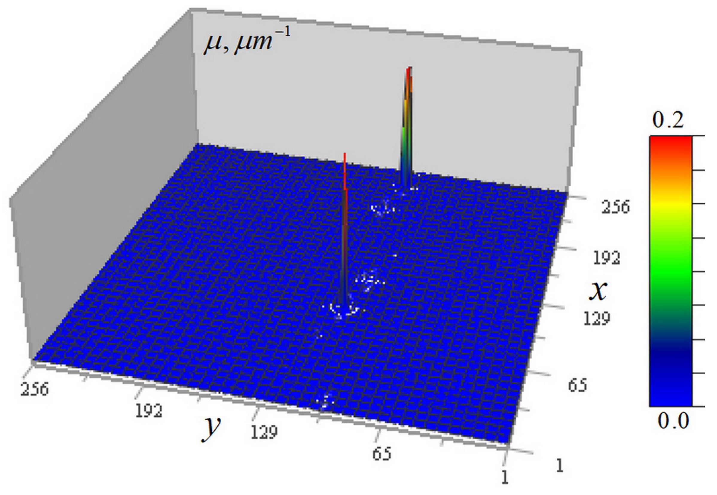
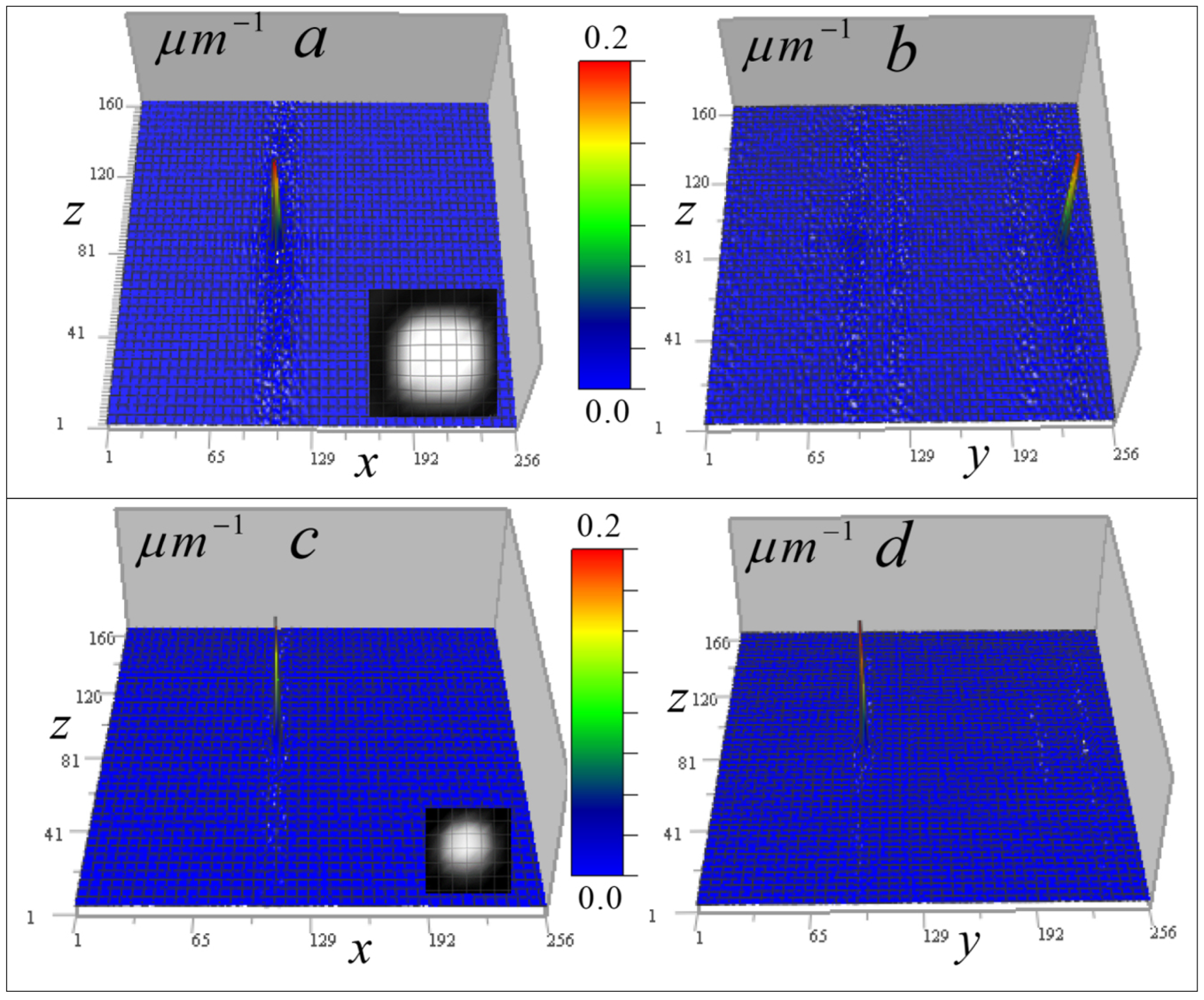
Figure 4 shows the results of numerical simulation of algorithms (9) and (10) for test inhomogeneities in a medium with a constant component
= 0.08 µm
−1 (the optical thickness of such a medium is
, and
). Inhomogeneities of the absorption coefficient were modeled: distributed inhomogeneity based on a Gaussian distribution with a Gaussian internal cavity
where
xc =
yc =
zc = 128 px,
σ1 = 4 px,
σ2 = 2 px (1 px = 50 nm); cube = 0.01 µm
−1 with dimensions 3 × 3 × 3 px at
xc = 64 px, and two 1-pixel inhomogeneities:
= 0.02 µm
−1,
= 0.01 µm
−1. These inhomogeneities have the same appearance in the
xy and
xz sections and are shown in
Figure 4 from two angles.
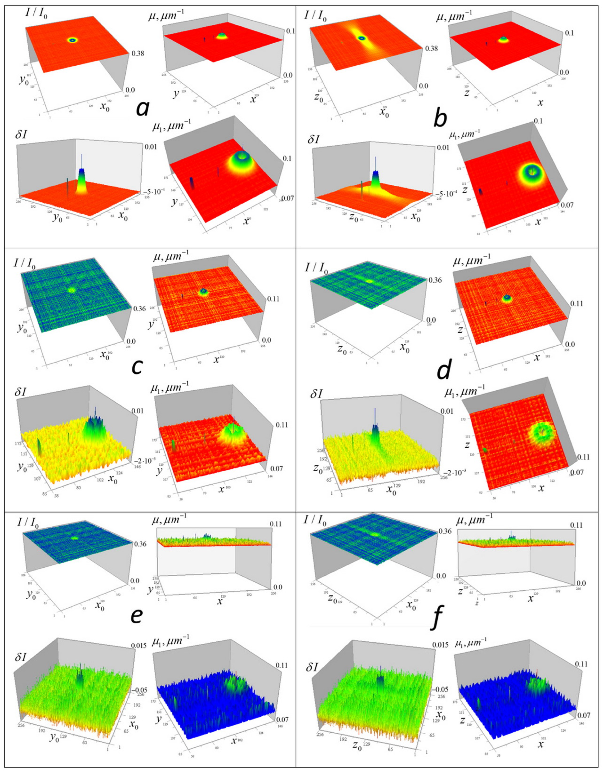
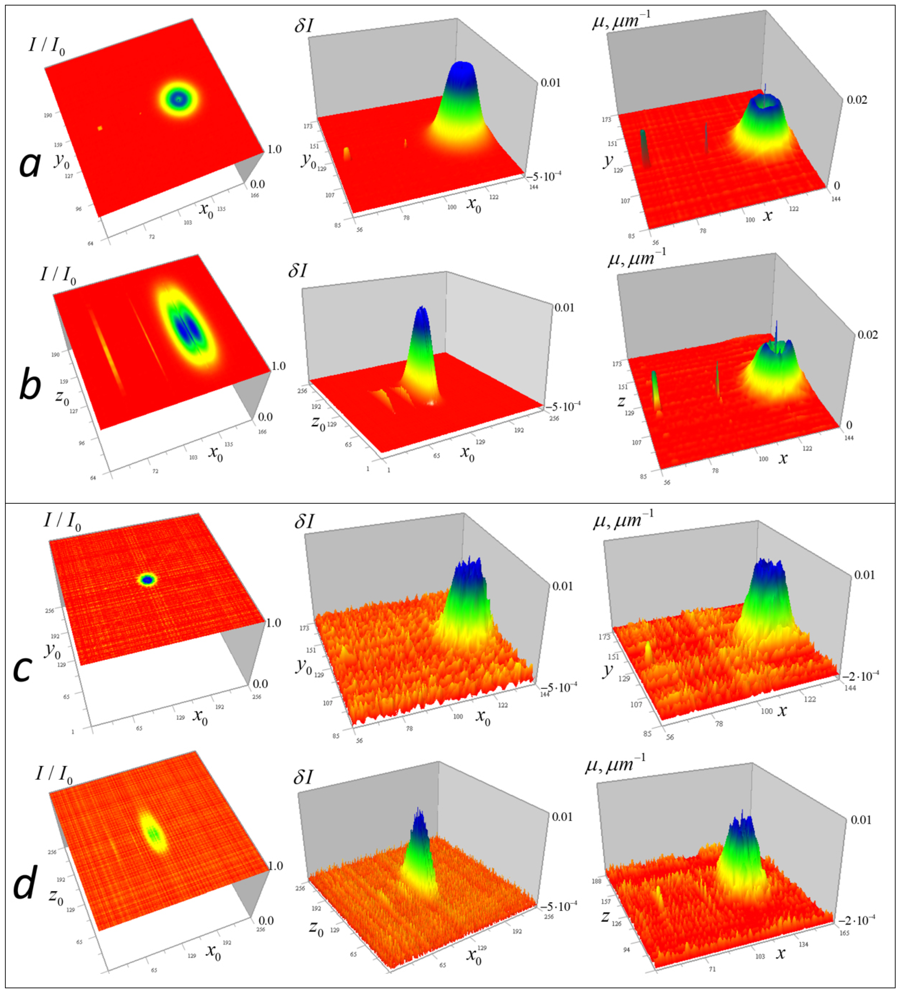
Figure 5 shows numerical simulation results obtained without regularization at simulated random error levels of σ = 1, 10, and 30% of the maximum value of the large Gaussian test inhomogeneity.
Figure 5 shows the full-scale (256 × 256) received signal distributions
with added random error and corresponding enlarged (128 × 128) distributions
of the left side of the tomography Equation (9), which displays the contribution of the test objects to the signal. It also shows the tomographic distributions of the absorption coefficient
of the test objects obtained from these data (in full-scale) and the contribution of the test objects to this distribution (128 × 128, above the level of the constant component
). The color scale was chosen for optimal distinguishability of inhomogeneities.
In
Figure 5, it can be seen that test objects make small contributions to the distribution of signal attenuation
compared to the constant component of the absorption coefficient
μ0. However, with small (1%) error in
(
Figure 5a,b), they are reproduced almost accurately, including a small cube with sharp edges, an internal cavity in a Gaussian function solid object, and two 1-pixel inhomogeneities—one inside this cavity and another outside the Gaussian object. It is important to note that despite the significant signal blurring in the vertical plane (right column of
Figure 5), corresponding tomographic reconstruction results do not differ significantly from horizontal plane reconstructions over the wide data error range shown in
Figure 5.
In reconstructions obtained without regularization, errors appear almost proportional to the simulated random error levels, which confirms the correctness of the inverse problem formulation. As seen in
Figure 5e,f, even with a 30% error rate, the small cube and 1-pixel objects are reconstructed well—the method implements such resolution for inhomogeneities whose signal exceeds noise level. However, numerical simulation results do not yet permit conclusions about the same effectiveness in real diagnostics.
3.1.3. Cell Tomography with ×46 EUV Microscope
Experimental studies of this tomography method using ×46 EUV microscope were conducted on dried plant cells (lily of the valley stem,
Convallaria)—objects with a complex, multiscale internal structure, sampled at 256 × 256 × 160 with a resolution of 140 nm. These cell reconstructions by the weak absorption approximation algorithm were presented in [
14], enabling comparison with new algorithm results for inhomogeneities in the absorbing medium (9–13).
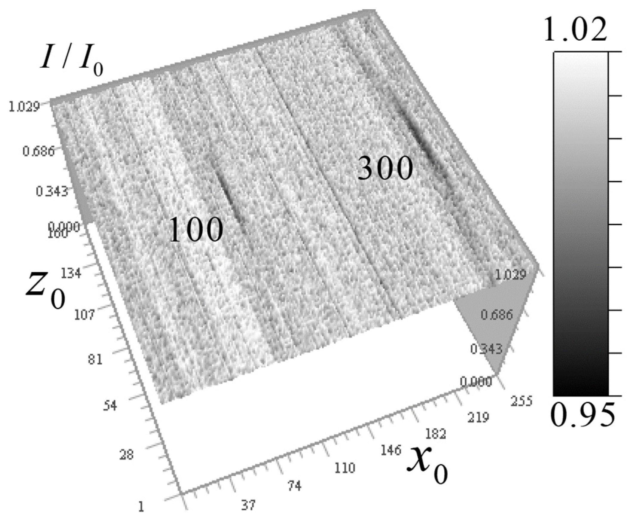
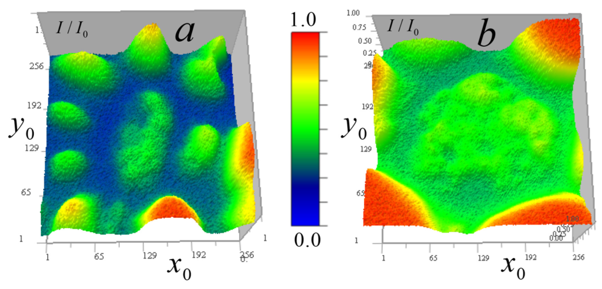
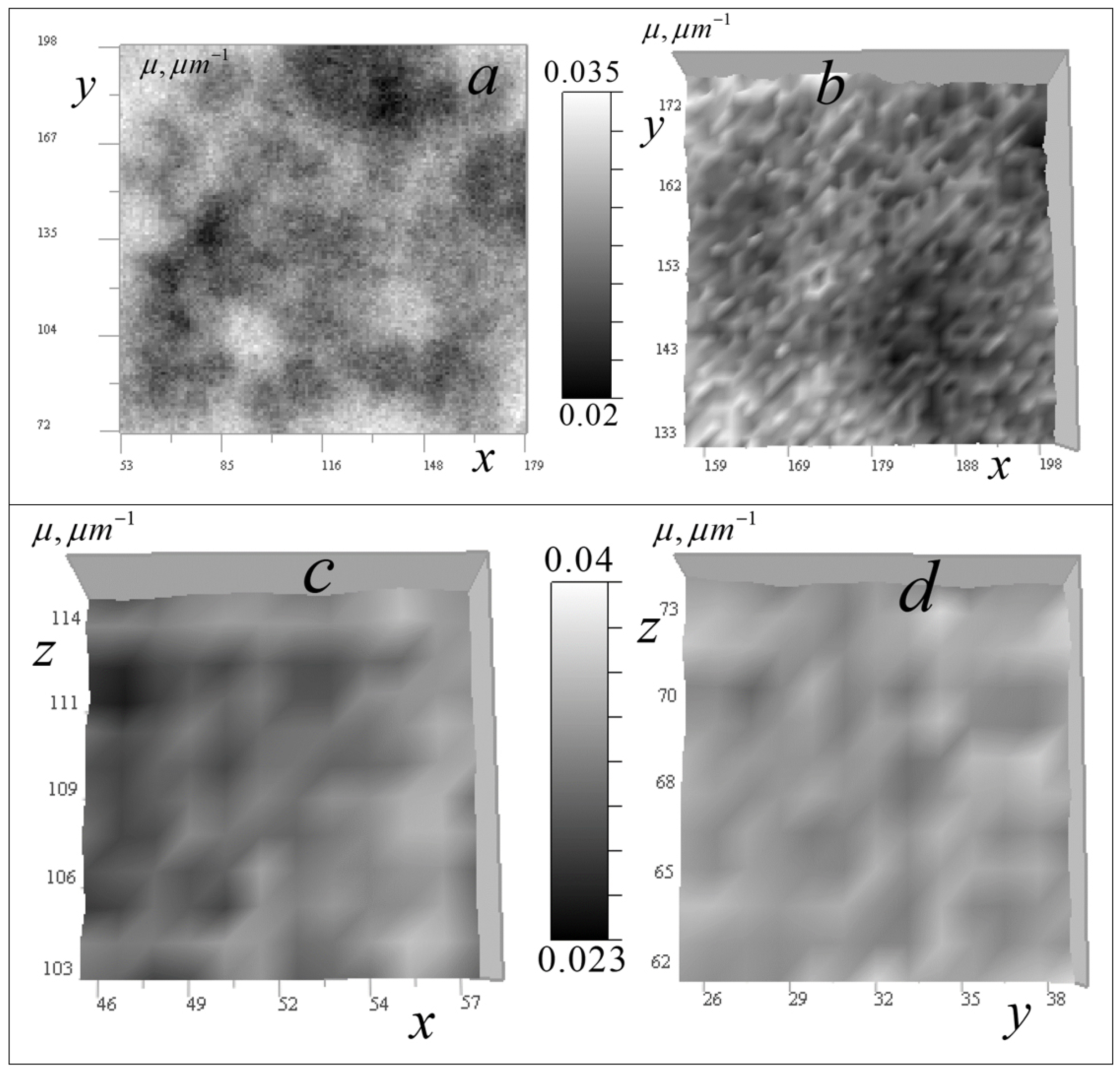
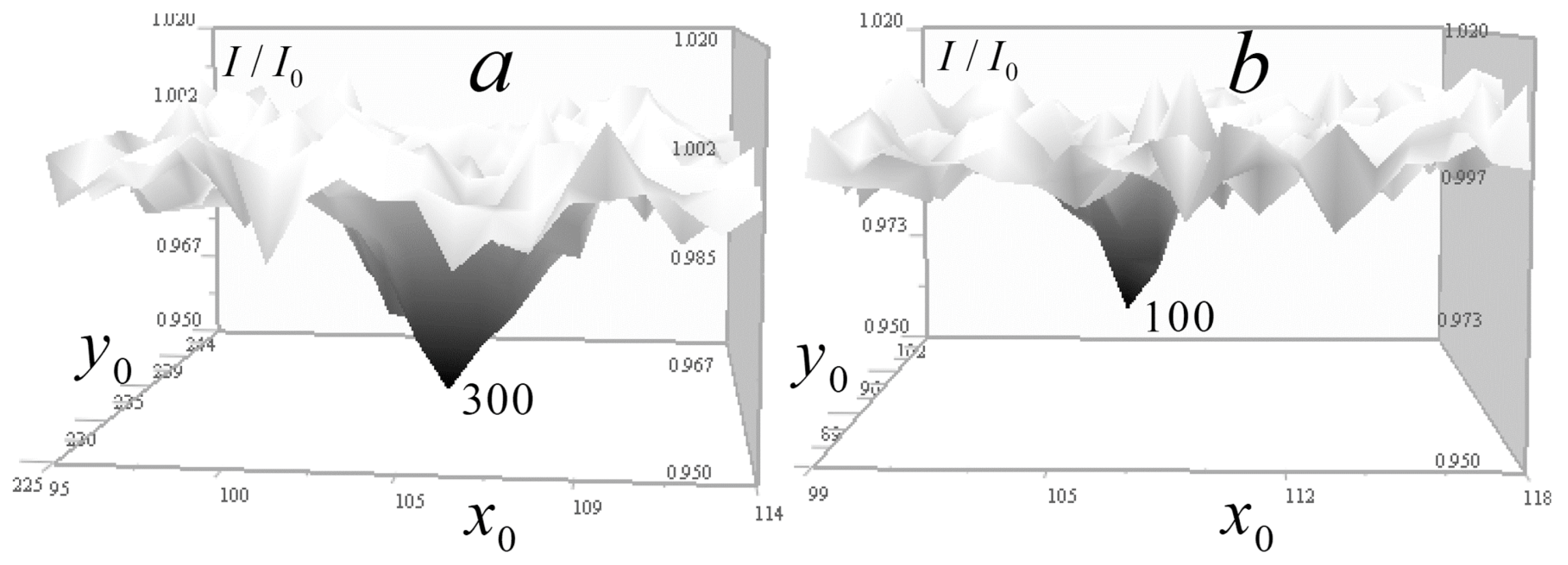
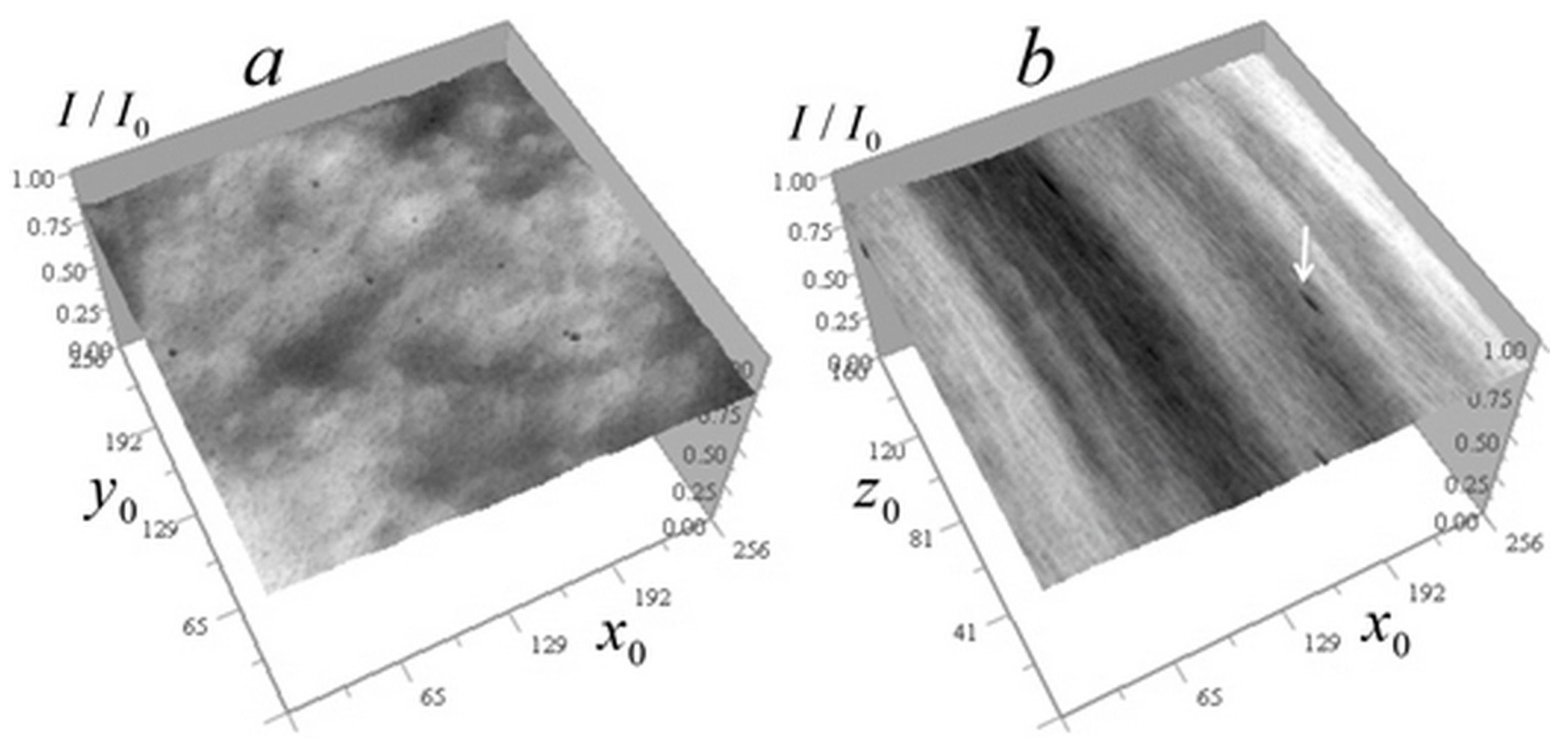
Figure 6 shows the measured signal distribution from two cells in the horizontal plane.
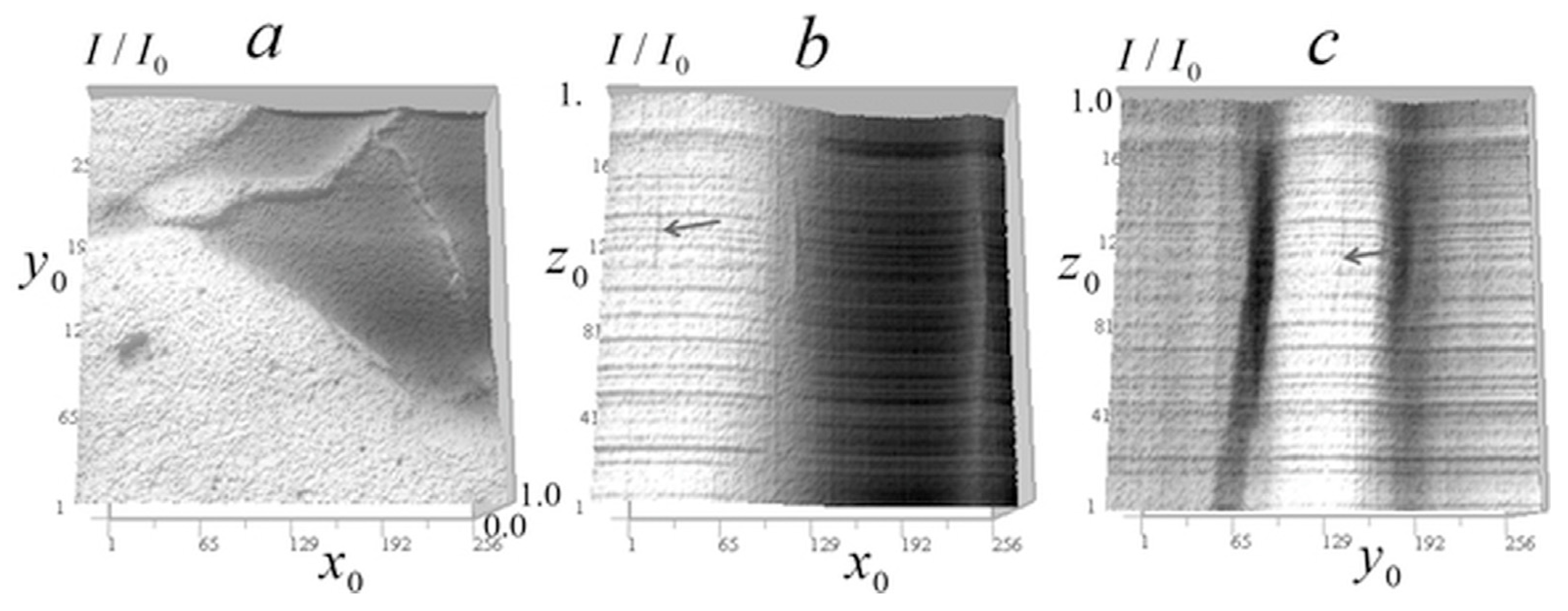
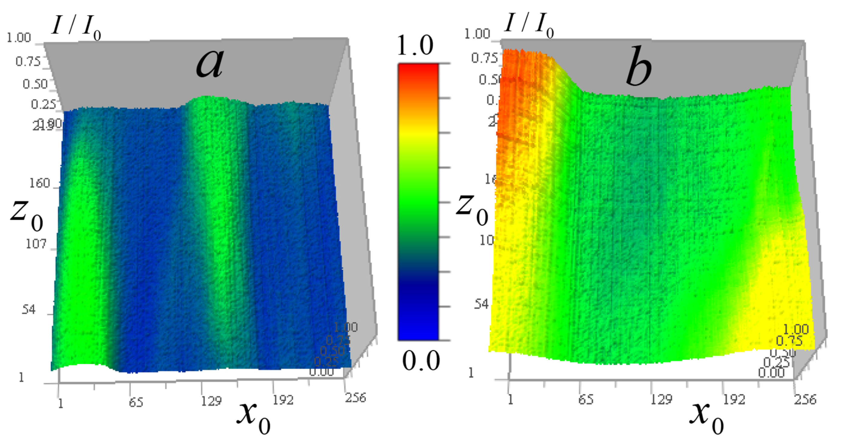
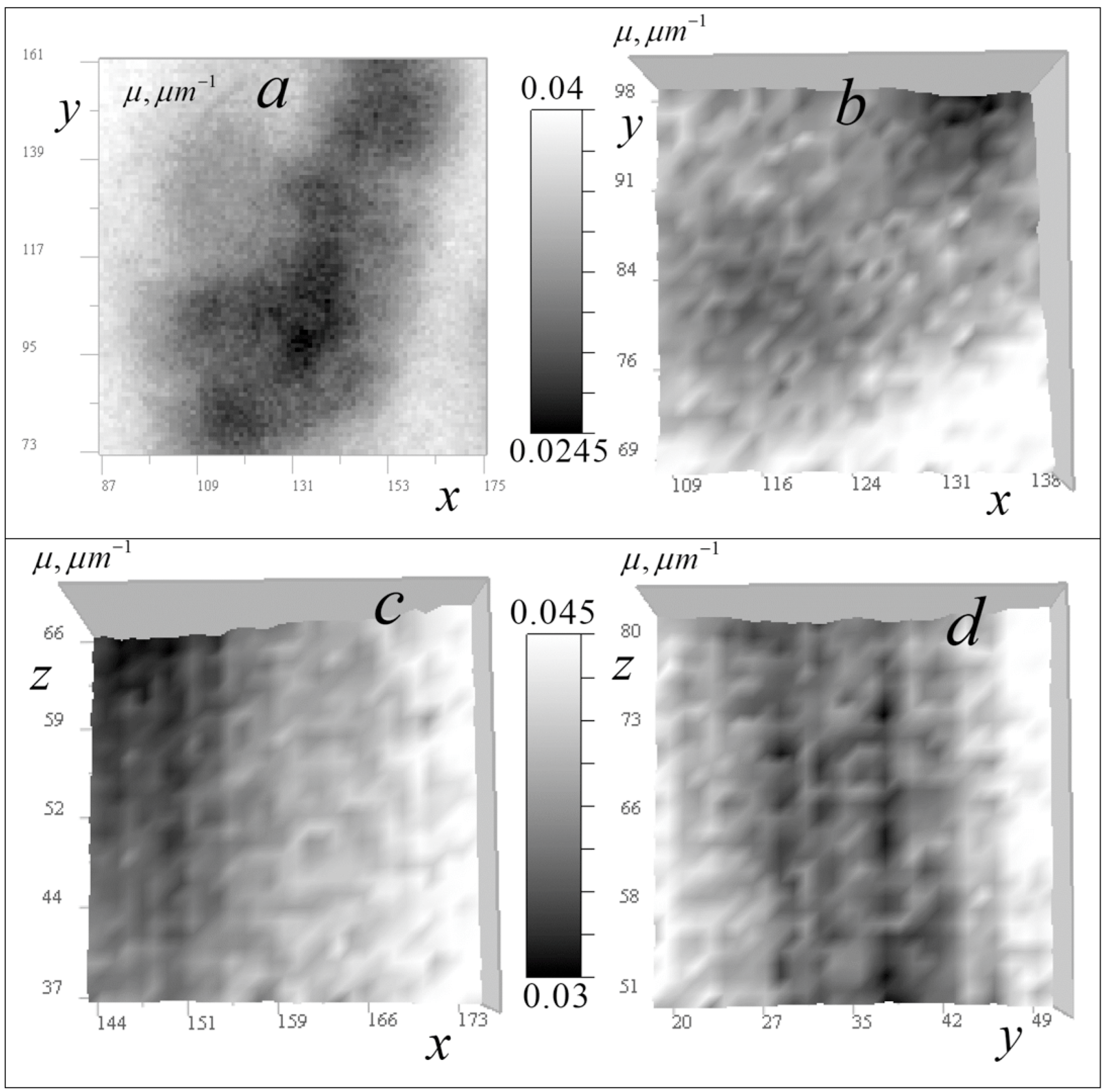
Figure 7 shows these cells in the vertical plane.
Figure 6 and
Figure 7 demonstrate that cell
B has generally higher transparency and more uniform distribution than cell
A. In the cell
A central region, the lowest vertical absorption can be observed at the point
. This enables determining a constant absorption coefficient component for this region by relative signal attenuation at this point
= 0.0245 μm
−1. Therefore, at this point
= 0.
The cells in
Figure 7 have vertical layers with nearly uniform vertical attenuation
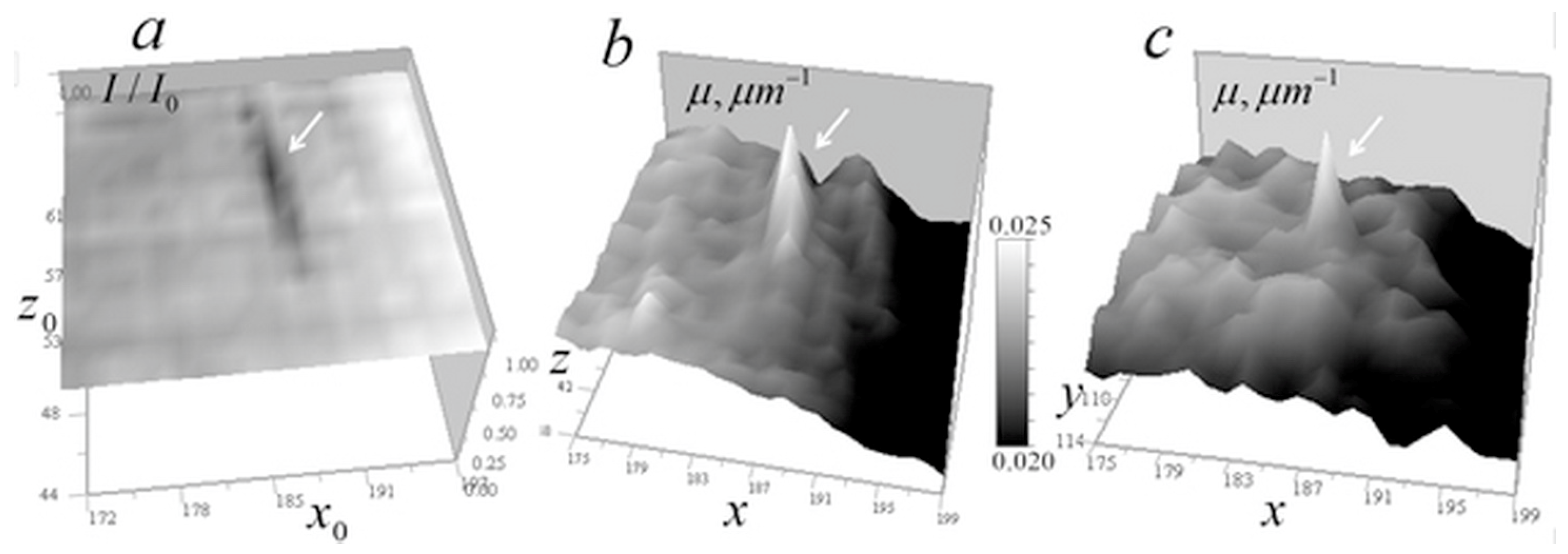
, and therefore, the corresponding distribution of the absorption coefficient is close to a constant value. This enables determining the absorption coefficient of the layer, selecting a second calibration point for the reconstruction result (13) and adjusting the kernel focus based on the known absorption in this layer. In cell
A, a point (97, 170, 108) was selected for calibration in an almost vertically homogeneous cell area with relatively high absorption, for which
= 0.0449 µm
−1. The distribution below and above the point is nearly uniform—variations are insignificant (the standard deviation on the vertical line passing through this point is less than 2%). For cell
B, the value of the constant component determined by the minimum absorption
(205,107,174) = 0.624 in a homogeneous layer was
= 0.0157 µm
−1. A second calibration point (87, 53, 174) was selected from a layer with relatively high absorption in this region
= 0.0313 µm
−1.
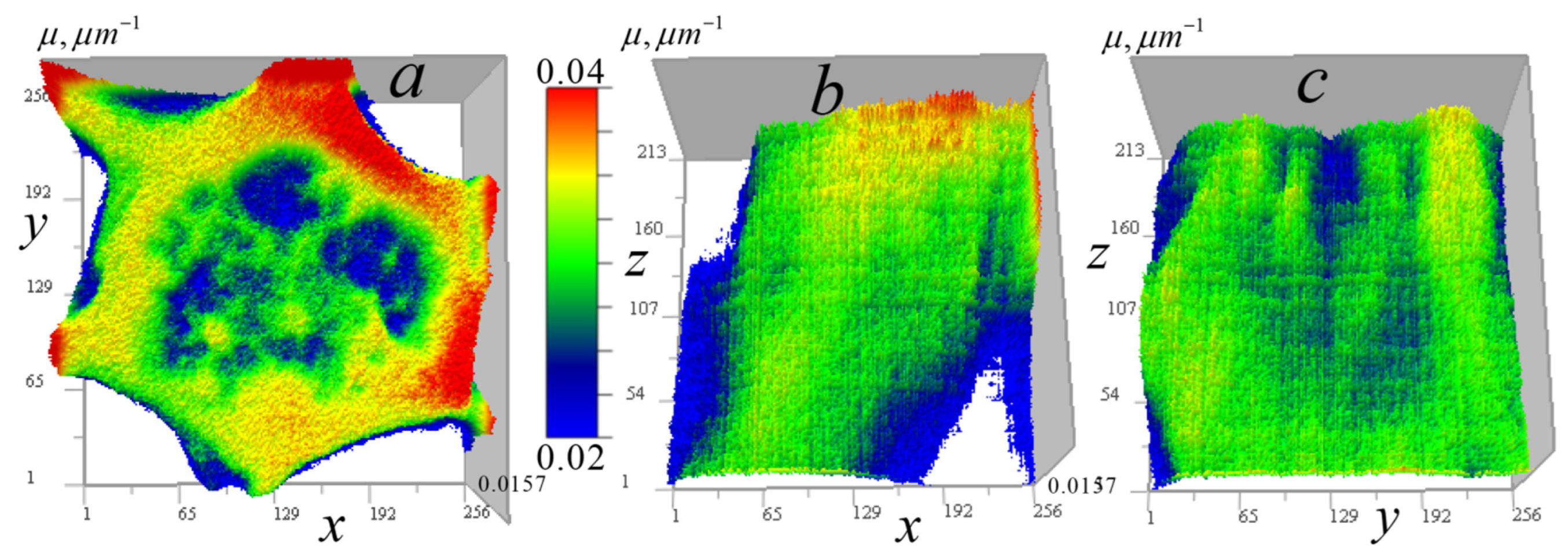
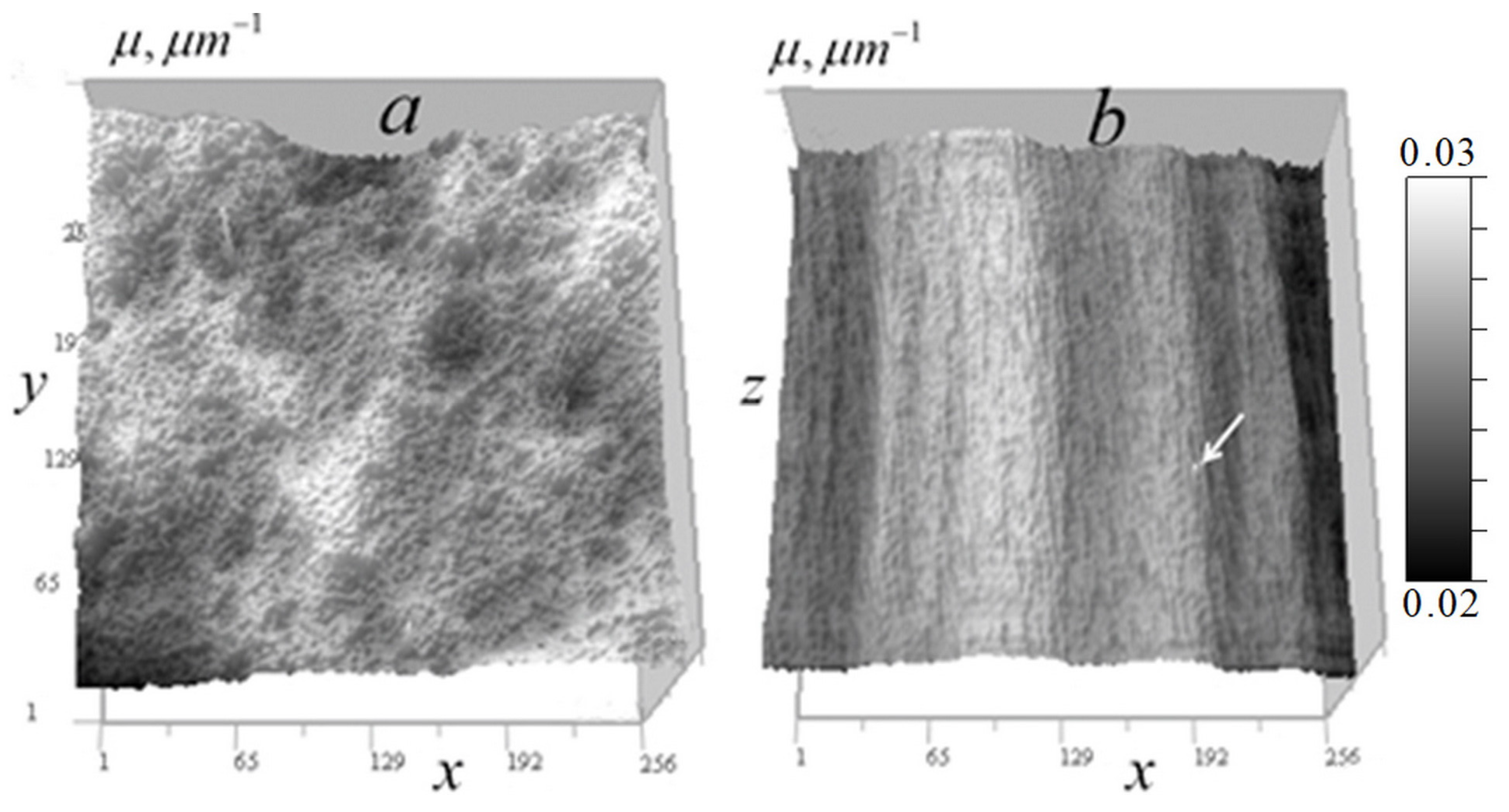
In
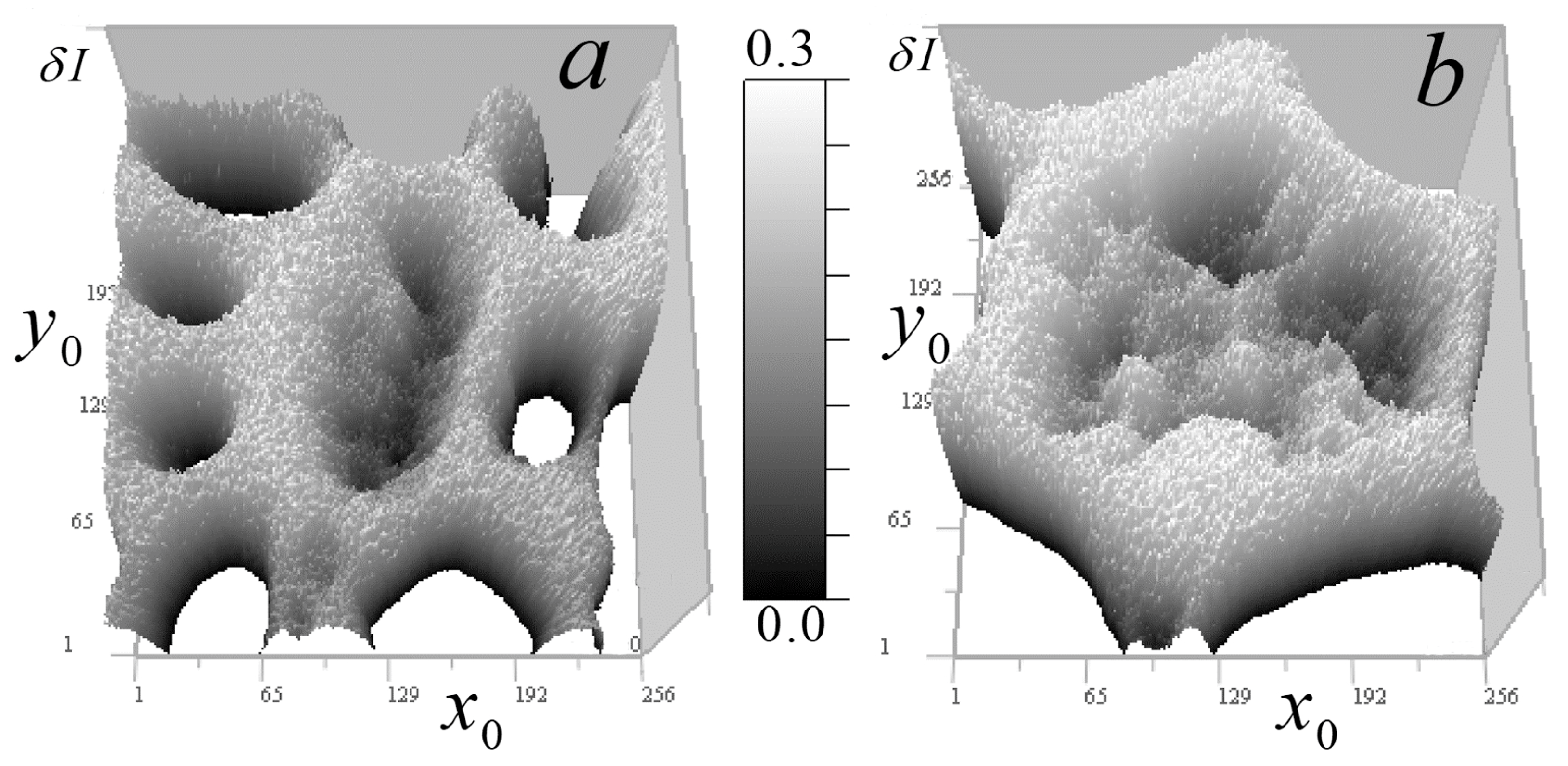
Figure 8, one can see the signal regions highlighted above the constant component, which allows one to obtain more accurate quantitative data on small inhomogeneities in these regions.
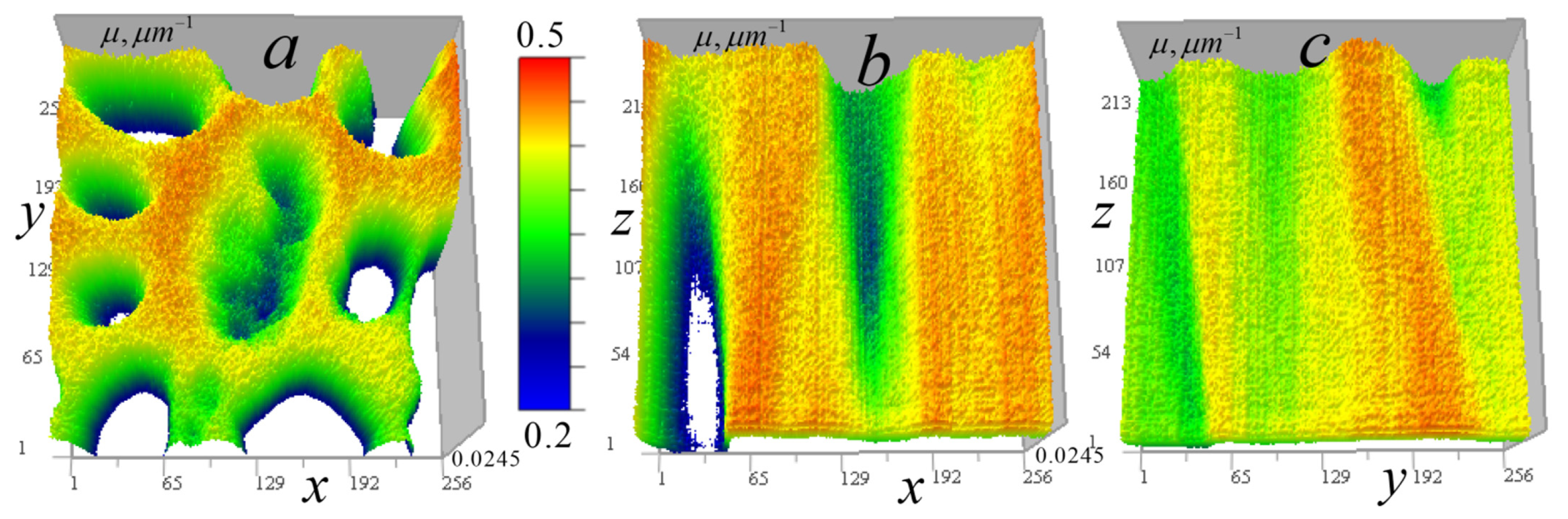
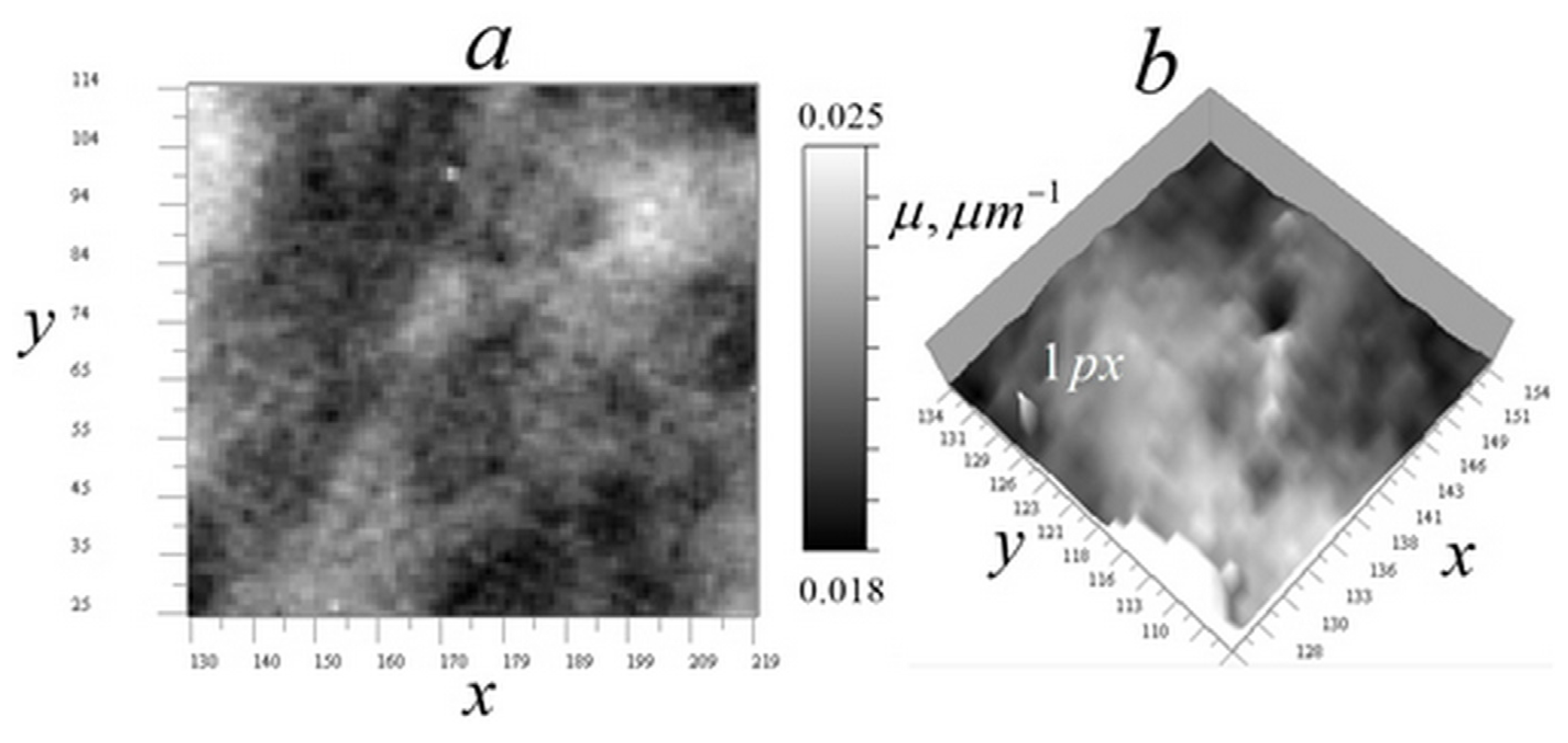
Figure 9 shows the results of the reconstruction of the absorption coefficient distribution in both horizontal and vertical tomographic sections for cell
A.
In
Figure 10, the results of the tomography are shown at a reduced scale, demonstrating, in comparison with the results of [
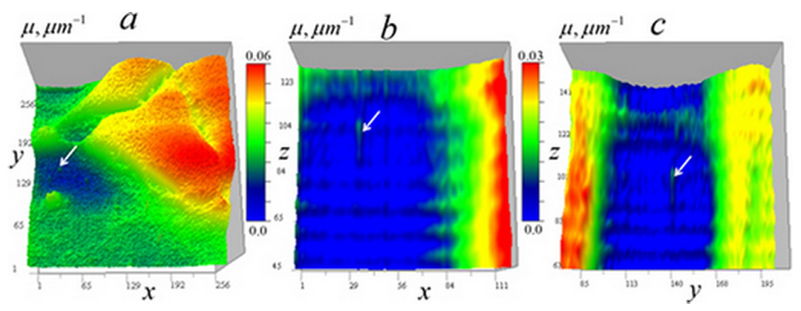
14], a greater depth of contrast and improved detail of the smallest distinguishable organelles visible in areas of relative transparency. Numerous small ring-shaped absorption inhomogeneities with dimensions 0.003–0.007 micrometers are visible. Presumably, they are shells of spheroidal bodies with a thickness of 0.15–0.3 μm, more transparent contents (by 0.0005–0.003 μm
−1), and transverse dimensions of 0.3–0.7 μm. Rings shown in the horizontal section in
Figure 10a,b are, on average, smaller than rings shown in vertical sections in
Figure 10c,d.
Figure 11 shows the results of the tomographic reconstruction of the absorption coefficient distribution in cell B, both horizontally and vertically (in vertical sections passing through calibration points with relatively high absorption).
Figure 12 shows cell
B tomography results at a reduced scale.
In
Figure 12, tomography results also show an improvement in the detail of the smallest organelles compared to reconstructions in [
14]. In the horizontal section of a relative transparency area in cell B (
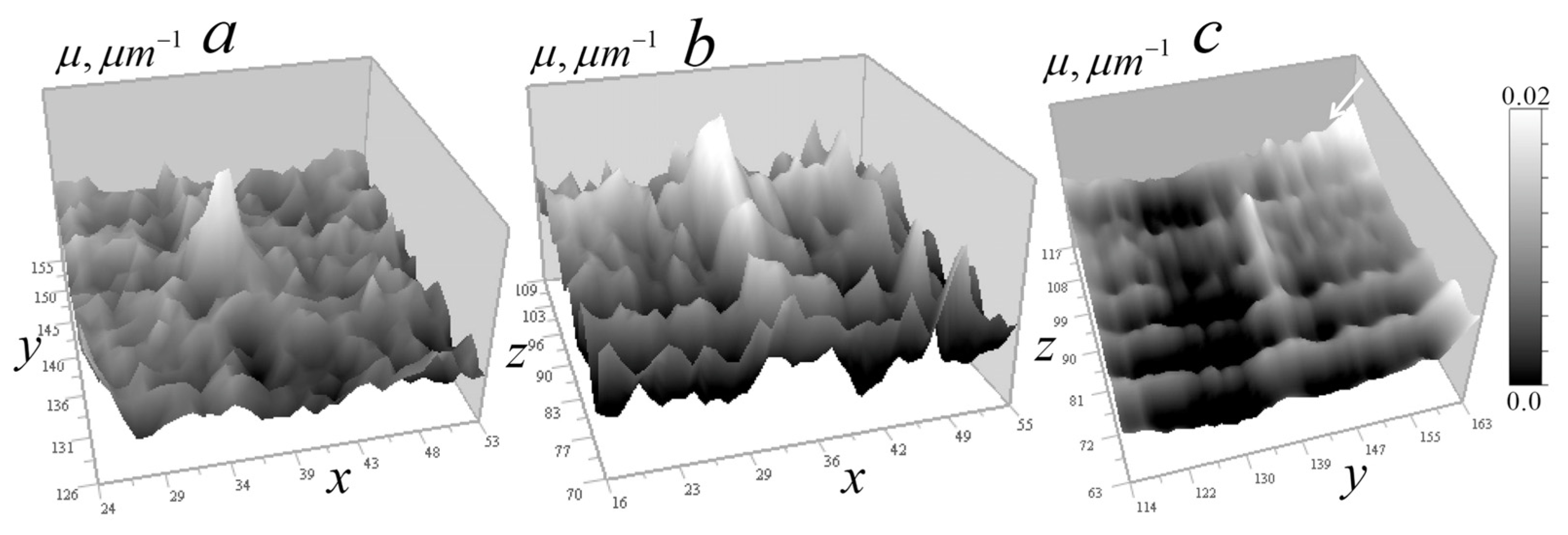
Figure 12a), ordered star-shaped formations and various-sized ring structures are visible.
Figure 12b shows a small area with accumulation of the smallest annular bodies, with linear dimensions ranging from 0.3 to 0.7 μm with a shell thickness ranging from 0.15 to 0.3 μm, which were not found in the reconstructions [
14]. The absorption coefficient variations in these bodies are comparable to those seen in the reconstruction shown in
Figure 10b.
Figure 12c,d show two vertical sections of the largest ring formations, with transverse dimensions of approximately 0.7 μm, shell thicknesses up to 0.3 μm, and cavity dimensions ranging from 0.3 to 0.45 μm. In the cell in
Figure 12c, the ring organelles’ absorption range is 0.0279–0.0291 μm
−1 and inner cavity is 0.0256–0.0267 μm
−1, i.e., the shell’s contribution to absorption is 0.0023–0.0035 μm
−1. There is also an internal inclusion with absorption of 0.0273 μm
−1. In the cell shown in
Figure 12d, absorption is higher: ring organelles’ ranges are 0.0312–0.0326 μm
−1, cavity is 0.0300–0.0308 μm
–1, and the contribution from the shell is less than 0.0004–0.0026 μm
−1. There is a small inclusion with absorption of 0.0306 μm
−1 that is not easily visible.
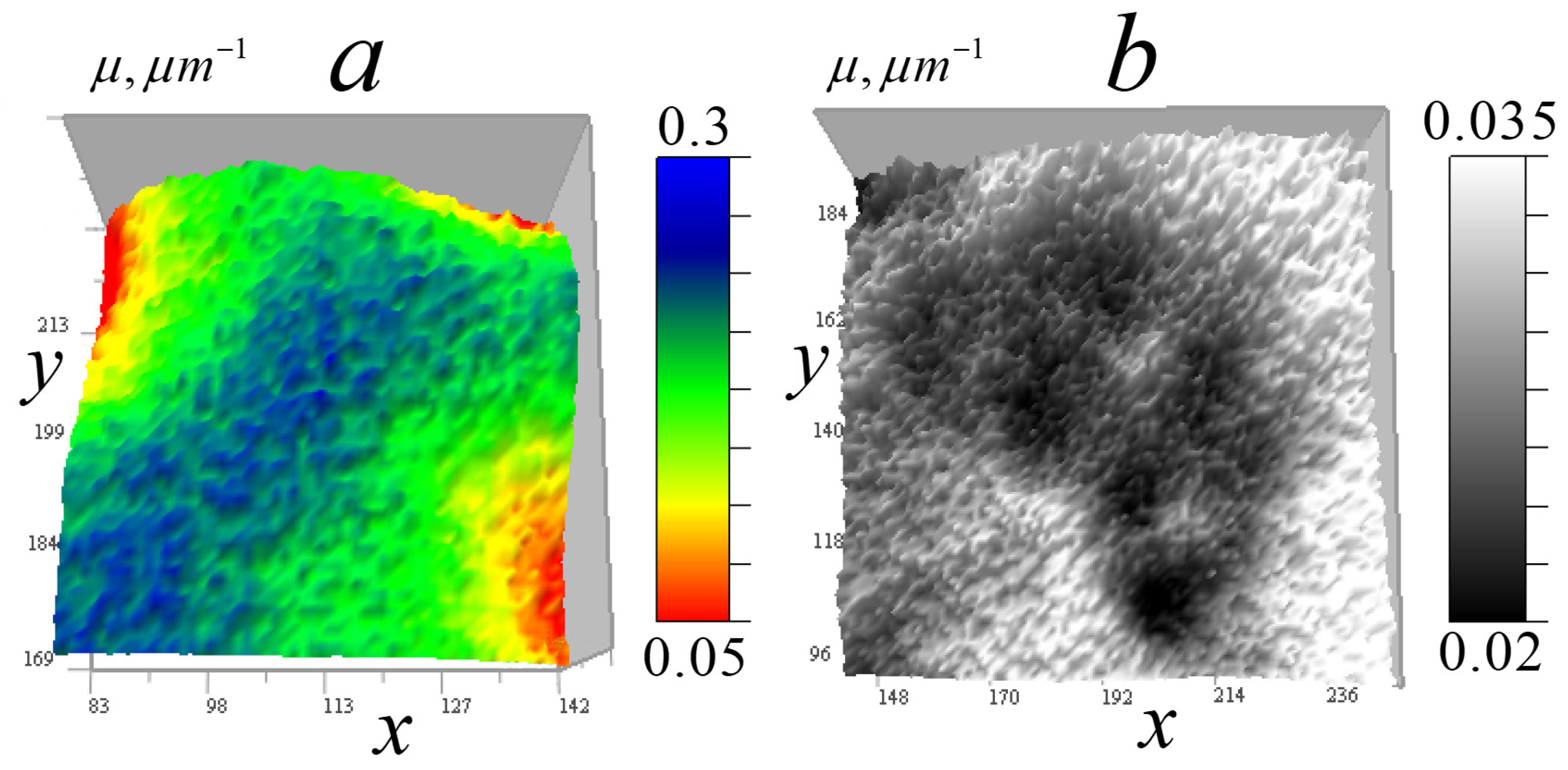
Figure 13 shows two reconstructions for cells
A and
B, respectively. Such structures were not resolved in [
14] using the algorithm in the weak heterogeneity approximation.
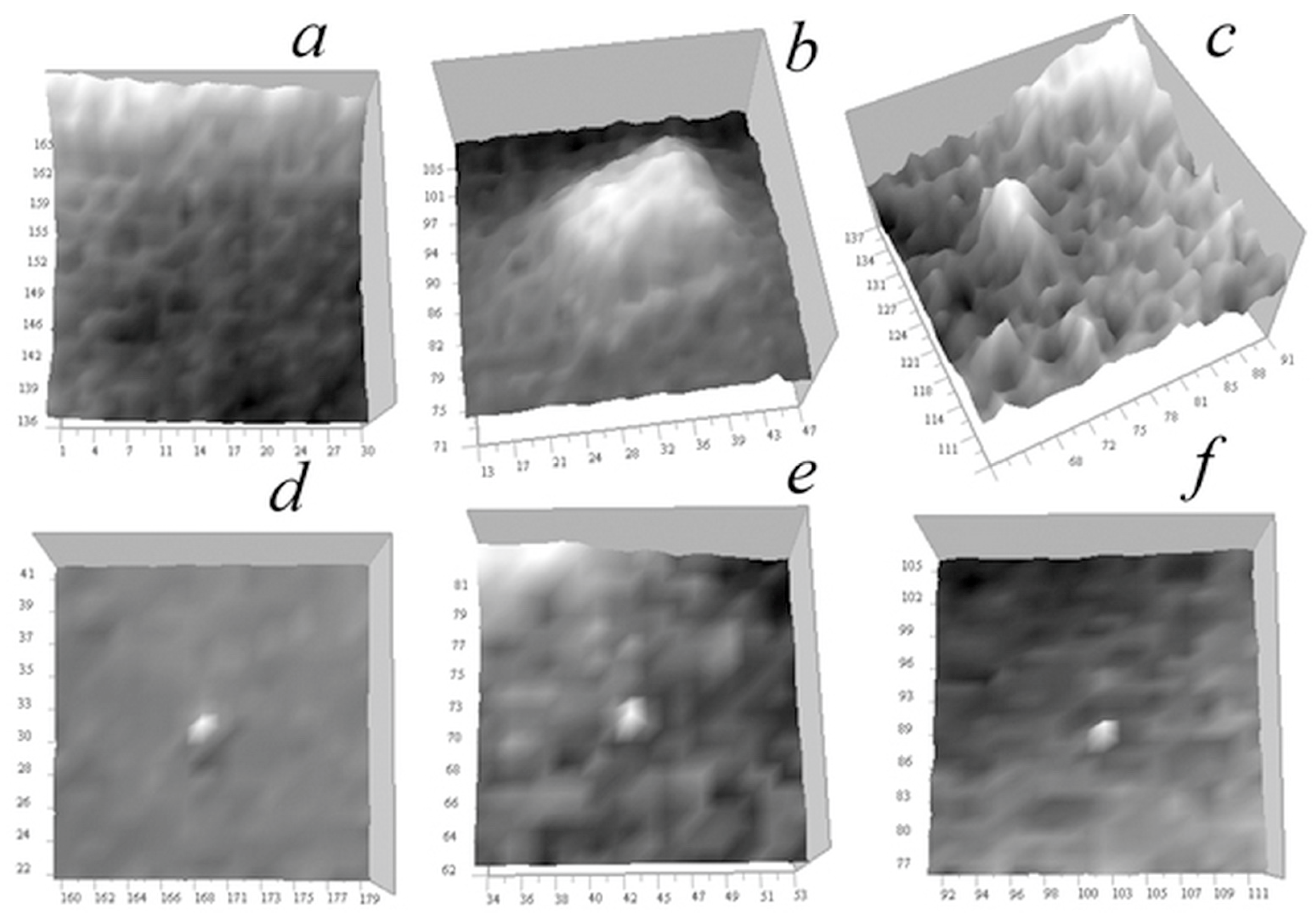
Using the selected color scale, ring-shaped structures (some with absorbing nuclei) against an increased absorption background (~0.2 μm
−1) were revealed in cell
A. The absorption coefficient in the nuclei exceeded that of the more transparent environment by 0.001–0.003 μm
−1. By choosing a contrast in the tomogram of cell
B, thin details of large-scale star-shaped organelles can be identified. Such details were indistinguishable in reconstructions obtained in the small absorption approximation [
14].
Thus, the tomograms in
Figure 9,
Figure 10,
Figure 11,
Figure 12 and
Figure 13 reveal the complex internal structure of the absorption coefficient distribution within cells—quantitative information inaccessible to optical diagnostic techniques, certainly of interest to biologists. The cellular structure in the images contains localized elements of varying scales. The ring formations, which are presumably parts of spherical bodies in the cell, are of particular interest. The resolution of the presented method enables detailed analysis of these small intracellular structures. Results demonstrate that the tomography algorithm provides a resolution of 1 pixel (140 nm) with the ×46 EUV microscope.