1. Introduction
The voxel-wise MR transverse relaxation rate,
, is sensitive to in vivo iron and myelin levels in the brain [
1,
2,
3]. It has been used broadly to study brain development and neurodegenerative diseases in humans and mouse models associated with alternations in myelin and iron content [
4,
5,
6,
7,
8,
9,
10,
11].
mapping is typically achieved by acquiring multi-echo gradient echo (GRE) images, followed by voxel-wise mono-exponential fitting of the signal decay. In the presence of iron and myelin, the magnetic susceptibility variations induce microscopic and mesoscopic field inhomogeneities in a voxel, resulting in accelerated signal decay and an increase in
. However, due to macroscopic voxel sizes,
values become inaccurate due to macroscopic field inhomogeneities (Δ
B0), such as regions near air-tissue interfaces. This considerable Δ
B0 effect leads to additional signal decay and overestimation of the
[
12]. Therefore, correcting for the Δ
B0 effect is necessary for accurate
measurement.
The Δ
B0 effect can be mitigated by using a small voxel size on a microscopic or mesoscopic scale, but it is impractical due to the low signal-to-noise ratio (SNR) [
12,
13]. For GRE images with a high in-plane resolution but thicker slices such as in a typical two-dimensional (2D) acquisition, the Δ
B0 effect is predominant along the z-direction [
12,
14]. Many methods have been proposed to correct for the z-direction Δ
B0 effect on
measurement [
14,
15,
16,
17,
18,
19,
20,
21,
22,
23,
24,
25]. By assuming that the z-direction Δ
B0 is linear, the correction can be performed using one of the following methods: (1) adding a z-direction gradient to compensate for Δ
B0 [
14,
23]; (2) combining images from multiple acquisitions with incremental z-direction gradients [
15,
24,
25]; or (3) applying a tailored RF excitation pulse [
26] to reduce the intra-voxel spin dephasing due to Δ
B0. Alternatively, the correction can be performed through postprocessing [
16,
17,
18,
19,
20,
21,
22], which does not require pulse sequence modifications and can be generally applied to multi-echo GRE images. For an ideal slice profile and a linear Δ
B0, the Δ
B0 effect on the measured
can be corrected by applying a sinc weighting function to the monoexponential model [
17]. The corrected
(
) can be obtained by fitting the signal decay to the model with three parameters (
S0,
, and Δ
B0), referred to as the three-parameter model herein. Nonetheless, with an additional parameter (Δ
B0), the three-parameter model becomes more sensitive to noise at low SNR [
17], particularly when the number of echo images is small. An initial estimate of Δ
B0 based on phase images [
19,
20,
21,
22] or a separate data acquisition [
18] has been used to improve the
estimate, but this requires additional processing of phase images and may increase the scan time.
The purpose of this study is to present an improved postprocessing method to estimate the
in the mouse brain at 7T, which mitigates the cross-slice Δ
B0 effect while reducing sensitivity to noise. Based on the three-parameter model and an assumption of the smoothness of the Δ
B0 map, this study presents a two-stage fitting procedure to generate a less noisy estimate of
. The assumption of the smoothness of the
B0 and Δ
B0 maps has been utilized previously to reduce the noise effect on the Δ
B0 map for the
correction in the human brain and liver [
21,
22]. The novelty of the presented two-stage fitting procedure is that the Δ
B0 map is directly measured by fitting the magnitude images of the mouse brain, followed by the application of a smoothing filter to reduce the noise effects on the measured Δ
B0 map. By eliminating the need to process phase images, our method may help simplify the image processing workflow and provide more flexibility when phase images are unavailable or when obtaining an accurate estimate of
B0 maps through phase images is challenging. We demonstrate the feasibility of the presented method using in vivo mouse experiments and simulations.
2. Materials and Methods
2.1. In Vivo Measurements
MRI scans were performed following the protocol approved by the Institutional Animal Care and Use Committees (IACUC) at the University of Iowa (IACUC Protocol #2112263). A total of 8 healthy mice (1 female and 7 males; 2–6 months of age) were imaged on a 7 Tesla Discovery MR901 system (GE Healthcare, Milwaukee, WI, USA) using a body transmit coil and a 2-channel mouse brain receiver coil. The animals were sedated with isoflurane during the session. The imaging protocol included a vendor-supplied high-order B0 shimming routine, followed by a FIESTA sequence for anatomical T2-weighted images (in-plane resolution of 104 µm2, slice thickness = 160 µm, pixel bandwidth = 326 Hz, flip angle = 30°, TE/TR = 3/6.1 ms, number of averages = 4, and scan time of 9 min and 28 s) and a 2D multi-echo GRE sequence for the measurements (in-plane resolution of 156 µm2, slice thickness = 500 µm, 18 axial slices, pixel bandwidth = 244 Hz, flip angle = 60°, TR = 1000 ms, 6 TEs of 2.5–22.5 ms in increments of 4 ms, number of averages = 2, and scan time of 4 min and 24 s).
2.2. Data Fitting
Data fitting was performed on the magnitude images in DICOM format that were reconstructed using a vendor-supplied image reconstruction routine. The reconstructed images had an image voxel size of 78 × 78 × 500 µm3.
Voxel-wise fitting was performed using the proposed two-stage fitting procedure as described below:
In the first stage of fitting, the signals in each image voxel of six-echo GRE images were fitted with the three-parameter model [
17]:
where TE is the echo time of GRE images,
is the signal at TE = 0,
γ is the gyromagnetic ratio, and
(
is the constant z-direction gradient and
is the slice thickness). Due to the additional parameter (Δ
B0), the three-parameter model was sensitive to noise and generated noisy estimates of
γΔ
B0 and
. By assuming that the
γΔ
B0 is slowly varying on the x-y plane, a 2D Gaussian filter with a standard deviation (
σgaussian) of 390 µm, which was the length of five image pixels and around 2.5 times the in-plane image resolution, was applied to the
γΔ
B0 map to reduce the effect of noise and generate a smoothed
γΔ
B0 map (
γΔ
B0smooth).
In the second stage of fitting, given the γΔB0smooth map, the multi-echo GRE signals of each image voxel were divided by the sinc weighting function ()) in Equation (1) to remove the ΔB0 effect. Following the division, the signals were fitted by the monoexponential model to obtain the with a reduced sensitivity to noise.
For comparison, the monoexponential models were also fitted to the six-echo GRE signals to generate the
map without correction (
). All of the fittings were performed using the trust-region-reflective algorithm [
27] in Matlab R2023b (Mathworks, Inc.). The upper bound of
γΔ
B0 was set to 88 Hz given the longest echo time of 22.5 ms [
17]. The upper bound of
was set to 100 Hz.
Goodness-of-fit was evaluated using the reduced chi-square statistic (
) [
28].
quantifies the sum of squares of the residuals normalized by the degrees of freedom of the model and the noise variance of the GRE images. A 95% confidence interval was defined as
< 2.4 for a two-parameter model (the monoexponential model) and as
< 2.6 for a three-parameter model. The Akaike information criterion (AIC) [
29] was also used to compare the relative goodness-of-fit between the different fitting methods.
2.3. Regions of Interest Analysis
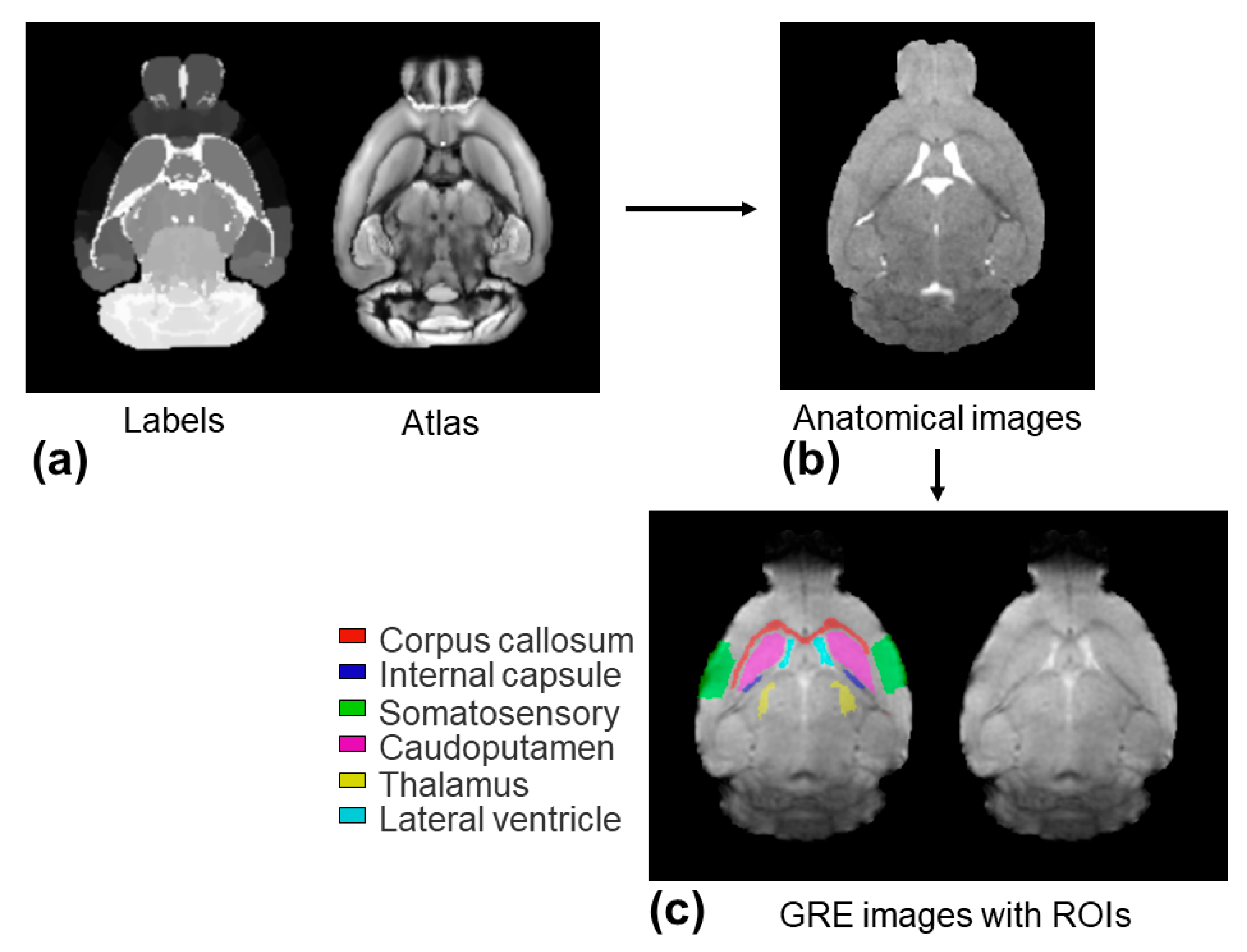
The regions of interest (ROIs), including the corpus callosum, internal capsule, somatosensory cortex, caudo-putamen, thalamus, and lateral ventricle, were selected to evaluate the
measurements. The ROIs were extracted from the structural labels of the P56 Mouse Brain atlas images [
30,
31,
32]. These structural labels were brought into the individual GRE image space using a non-linear co-registration between the P56 Mouse Brain atlas images and individual anatomical T
2-weighted images, followed by the linear co-registration between the individual anatomical T
2-weighted images and the GRE images. All of the image co-registrations were performed using ANTs [
32]. The ROIs on the GRE images were visually examined and adjusted for each mouse and were applied to the
maps. The within-ROI mean and standard deviation (SD) values of the
measurements were computed for each ROI. The image voxels with a poor fitting (
values outside the 95% confidence interval) were excluded from the ROI analysis.
2.4. Effect of the Smoothing Kernel Size
To investigate the effect of the smoothing kernel (σgaussian) of the 2D Gaussian filter applied to the γΔB0 map, four different values of the σgaussian, 234, 390, 546, and 702 µm, were used to smooth the γΔB0 map for the two-stage fitting procedure. The effect of the different smoothing kernels on was evaluated.
2.5. Statistics
Statistical analysis was performed to study (1) whether the fitting error, quantified by the AIC, of the monoexponential model is reduced by the application of the three-parameter model and two-stage fitting procedure; (2) whether the within-ROI SD of using the three-parameter model is higher than that of the of the monoexponential model due to the increased sensitivity to noise; and (3) whether the within-ROI SD of the is reduced by the application of the two-stage fitting procedure.
To address the above three questions, the one-tailed Wilcoxon signed-rank test was used for the comparisons, resulting in a total of 24 comparisons within the six ROIs. The significance level was adjusted for multiple comparisons using the false discovery rate [
33];
p-value < 0.0078.
2.6. Simulations
To study the noise effects on the
measurements in the presence of a cross-slice Δ
B0 effect, representative in vivo multi-echo GRE signals were simulated using Equation (1) with the parameters
of 30 Hz, 6 TEs of 2.5–22.5 ms in increments of 4 ms, and
of 50.
γΔ
B0 was increased from 1 to 45 Hz to reflect the range of measured γΔ
B0 in the selected ROIs of the in vivo mouse brain. Rician noise was added to the signals with an SNR of 50, the average measured SNR of the in vivo mouse brain’s 1st echo image. The procedure was repeated 1000 times to generate 1000 sets of noisy signals. One thousand sets of simulated noisy signals were fitted with the two-stage fitting procedure, monoexponential model, and three-parameter model as described in the
Section 2.2. For the two-stage fitting procedure, 1000 measurements of
γΔ
B0 were obtained through three-parameter model fitting and were smoothed to generate the
γΔ
B0smooth using a 1D Gaussian filter. The
σgaussian of the 1D Gaussian filter was set to 25 data points to match the square kernel
σgaussian (5 × 5 image pixels) used for the 2D Gaussian filter. Given the true values of
and
γΔ
B0, the accuracies of the measured
and
γΔ
B0 were evaluated using the root mean square error (RMSE). Moreover, the effect of the SNR on the
measurements was investigated by changing the SNR of the simulated signals from 20 to 100 and evaluating the accuracies of the measured
and
γΔ
B0 at different SNR levels.
3. Results
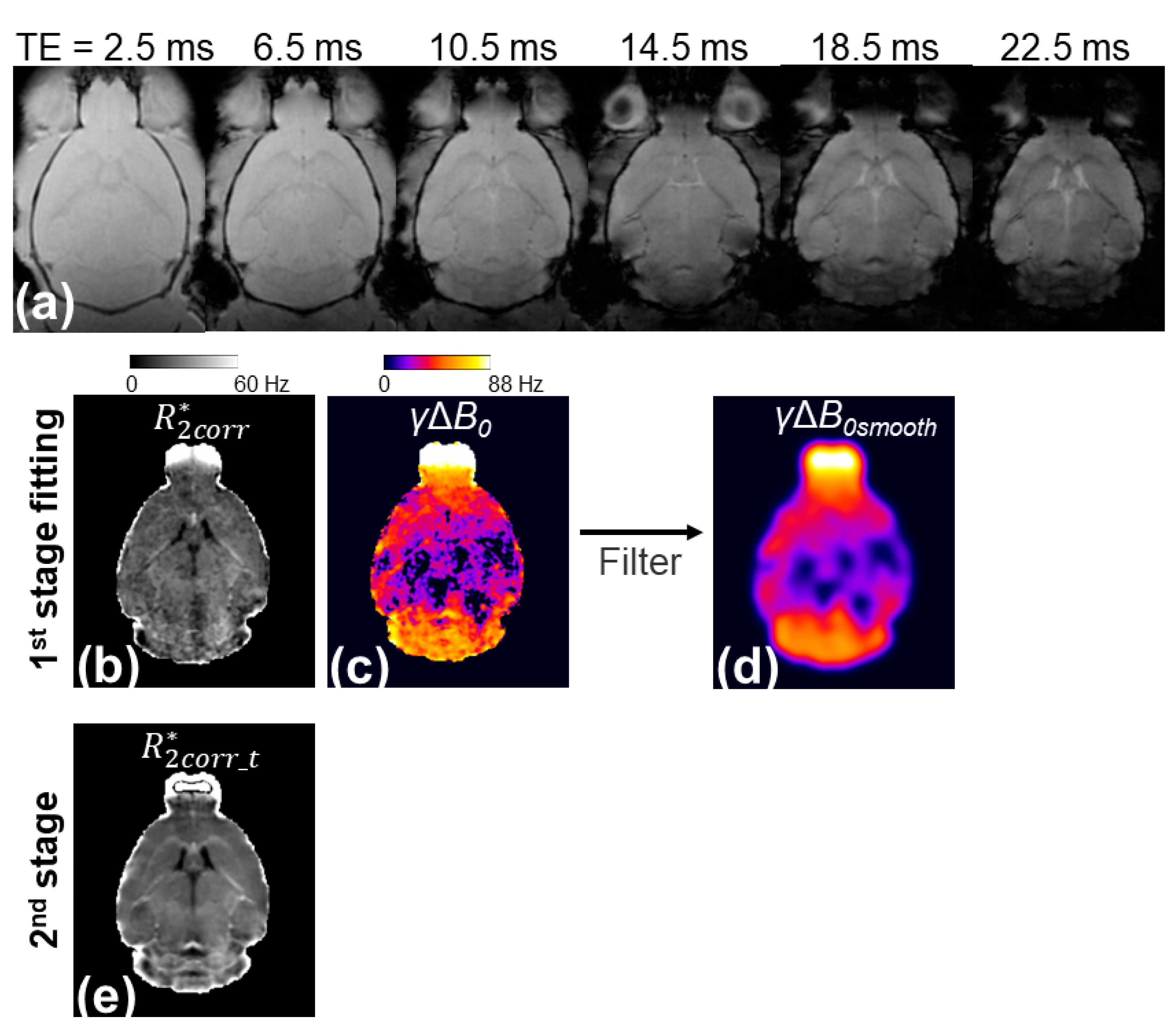
Figure 1 illustrates the workflow of the presented two-stage fitting procedure. The
γΔ
B0 map generated by the three-parameter fit showed a large Δ
B0 in regions with large magnetic susceptibility changes, such as the olfactory bulb, entorhinal cortex, and cerebellum, but it was noisy (
Figure 1c). A smoothing kernel was applied to the
γΔ
B0 map to reduce the noise effects while maintaining the spatial variation of Δ
B0 (
Figure 1d). The
γΔ
B0smooth map was applied to the three-parameter model to remove the Δ
B0 effect from the signal and reduce the unknown parameters from three to two, thereby generating a less noisy
map (
Figure 1e).
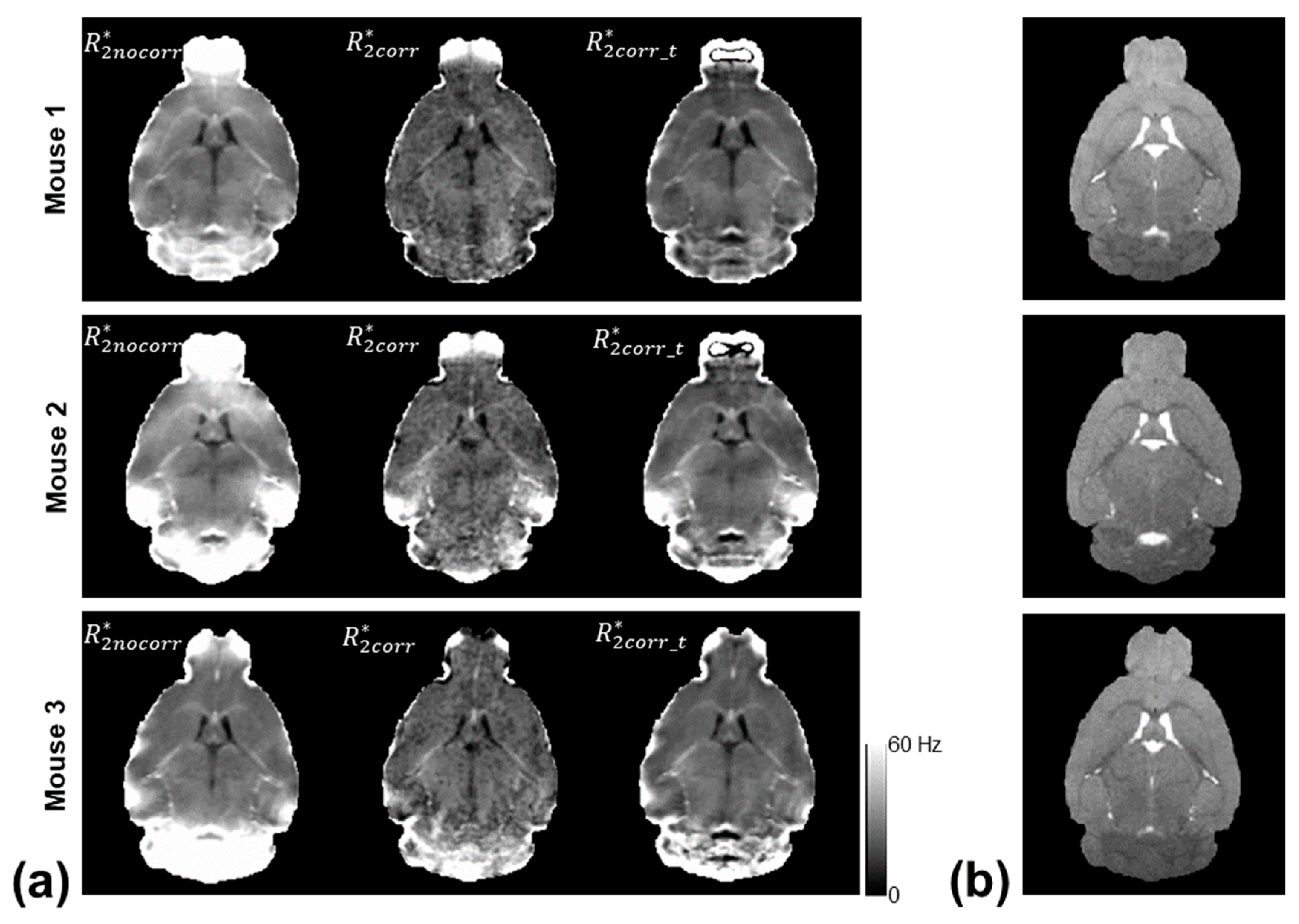
Figure 2 shows the computed
,
, and
maps of three mice using the monoexponential model, three-parameter model, and two-stage fitting procedure.
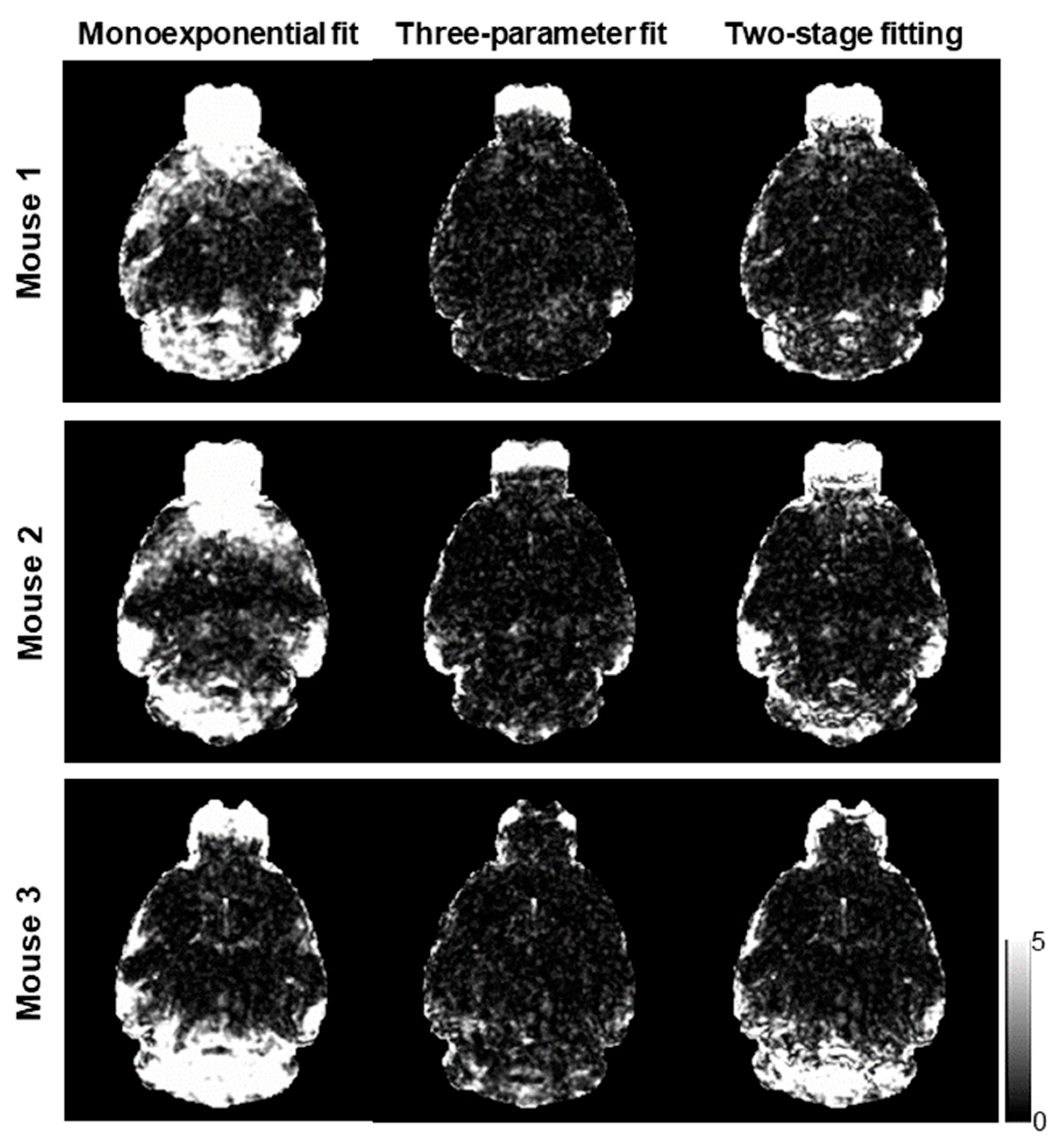
Figure 3 shows the corresponding
maps using the three fitting methods.
showed the Δ
B0-induced increases in the regions near air–tissue interfaces, where fitting residuals of the monoexponential fit were elevated. These Δ
B0 effects were consistently mitigated on the
and
maps. Furthermore, the noise effect on the
maps was mitigated on the
maps without compromising the contrast of the brain structure.
Further quantitative analysis on the six selected ROIs was achieved through an image co-registration workflow, as shown in
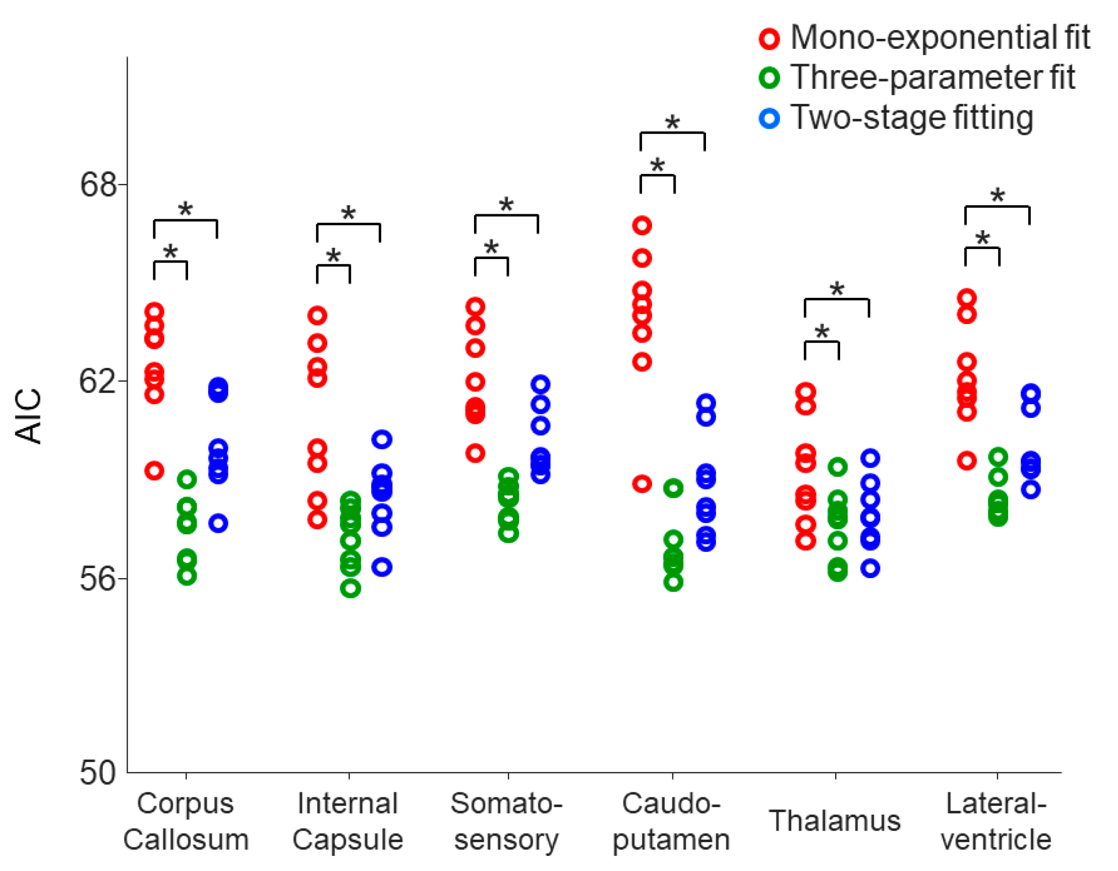
Figure 4. The AIC values of the monoexponential model were significantly reduced by using the three-parameter model and two-stage fitting procedure in all of the selected ROIs (
p = 0.0039–0.0078) (
Figure 5), suggesting that both the three-parameter model and two-stage fitting procedure are preferred to the monoexponential model in describing the data of the six ROIs.
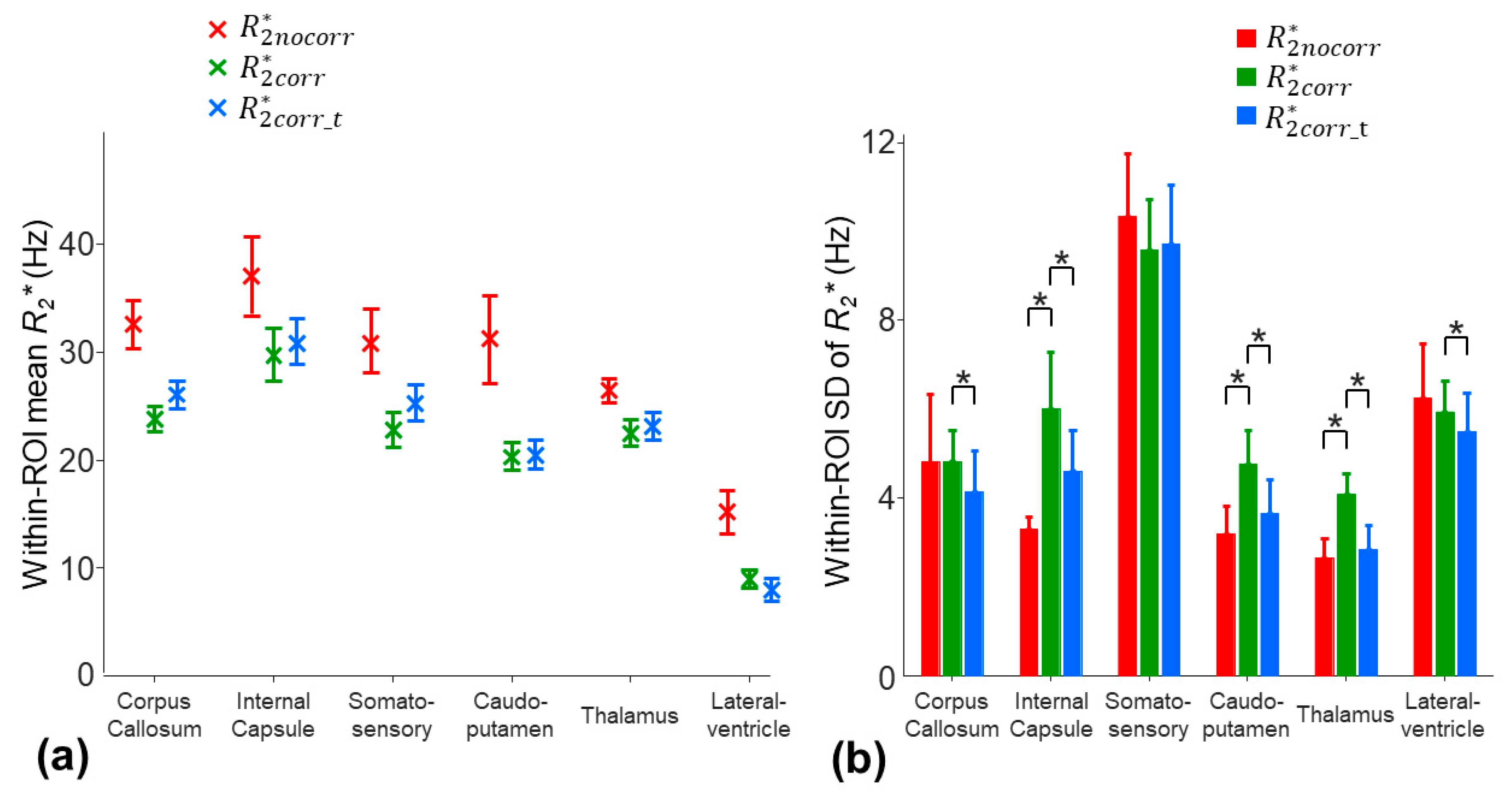
The averaged inter-subject SD of the mean
across the ROIs was decreased from 2.7 Hz to 1.4 and 1.5 Hz by using the three-parameter model and two-stage fitting procedure, respectively (
Figure 6a). Nonetheless, the within-ROI SD of the
using the three-parameter model was significantly higher than that of the
of the monoexponential model in the internal capsule, caudo-putamen, and thalamus regions (
p = 0.0039) (
Figure 6b). The higher within-ROI SD of the
was partially contributed by the increased noise sensitivity due to over-fitting. With the two-stage fitting procedure, the within-ROI SD of the
was significantly reduced by 7.7–30.2% in all the ROIs, except for the somatosensory cortex region (
p = 0.0039–0.0078) (
Figure 6b).
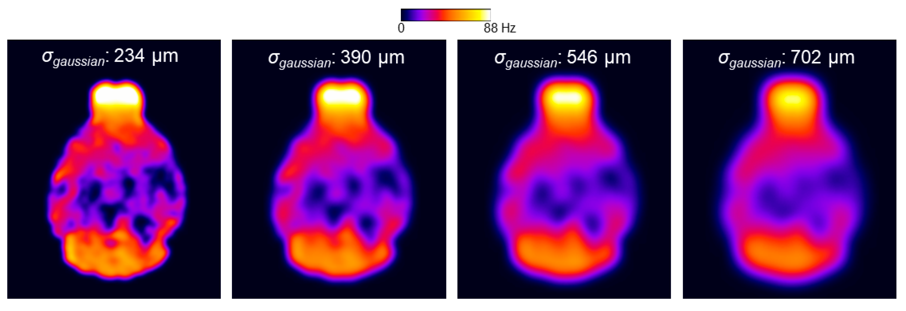
For the two-stage fitting procedure, the application of different smoothing kernels to the
γΔ
B0 map is illustrated in
Figure 7.
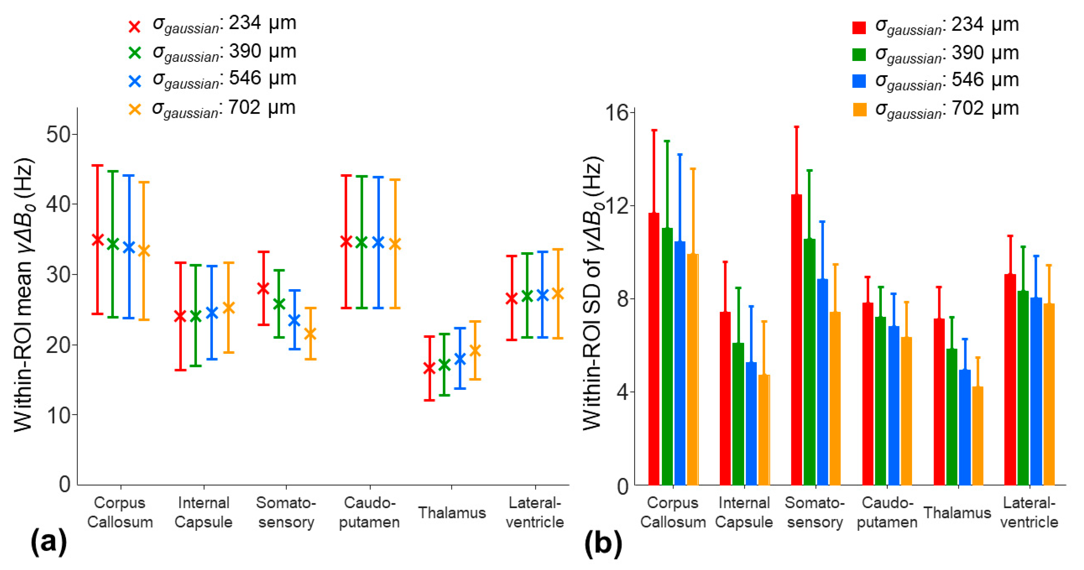
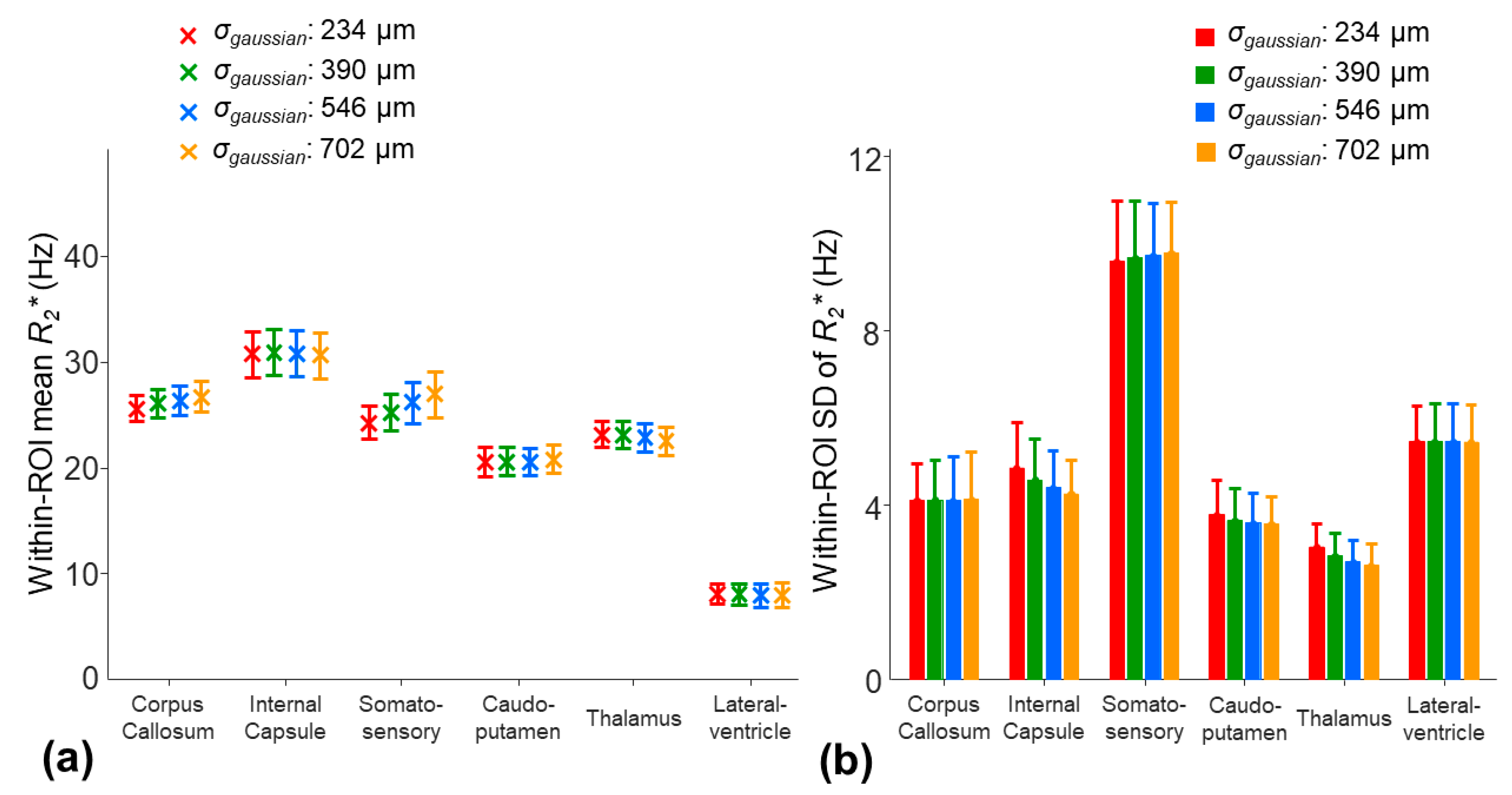
The application of a larger smoothing kernel (σ
gaussian increased from 234 to 702 µm) led to decreases in the within-ROI SD of the
γΔ
B0 in all the ROIs (
Figure 8b). Among the selected ROIs, the smoothing procedure had the largest impact on the mean
γΔ
B0 in the somatosensory region. The mean
γΔ
B0 was decreased by 6.5 Hz in the somatosensory region, whereas the changes in the mean
γΔ
B0 were less than 2.7 Hz in other ROIs (
Figure 8a). This potential underestimate of the
γΔ
B0 in the somatosensory cortex region using a larger smoothing kernel resulted in an increased mean
by 11.4% (
Figure 9a). In other ROIs, the changes in the mean
were less than 5%. On the other hand, a larger smoothing kernel led to the reduced noise sensitivity of the
. The within-ROI SD of the
was decreased by 12.3%, 5.6%, and 14% in the internal capsule, caudo-putamen, and thalamus regions, respectively (
Figure 9b).
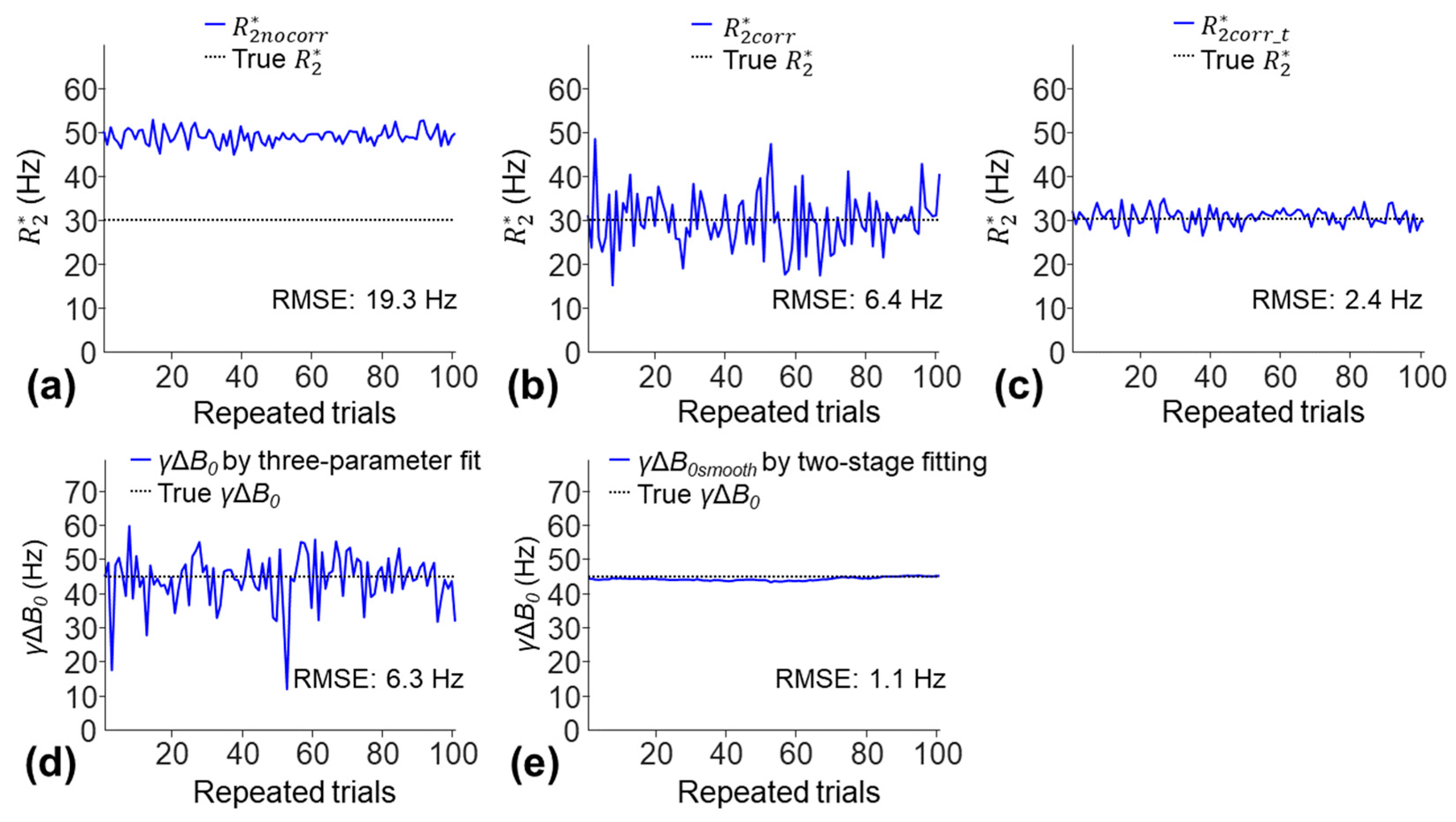
The simulations in the presence of a cross-slice Δ
B0 effect (true γΔ
B0 of 45 Hz) were performed to study the accuracies of the
and
γΔ
B0 measurements. The
had the highest RMSE of 19.3 Hz due to an overestimate of
(
Figure 10a). The
showed an improved estimate of
(RMSE of 6.4 Hz) but had a high SD due to increased noise sensitivity; the mean ± SD of
was 30.3 ± 6.5 Hz (
Figure 10b). The
was the most accurate (lowest RMSE of 2.4 Hz); the mean ± SD of
was 31 ± 2.4 Hz (
Figure 10c). The
γΔ
B0smooth measured using the two-stage fitting procedure was more accurate than the
γΔ
B0 measured using the three-parameter fit (RMSE: 1.1 Hz versus 6.3 Hz).
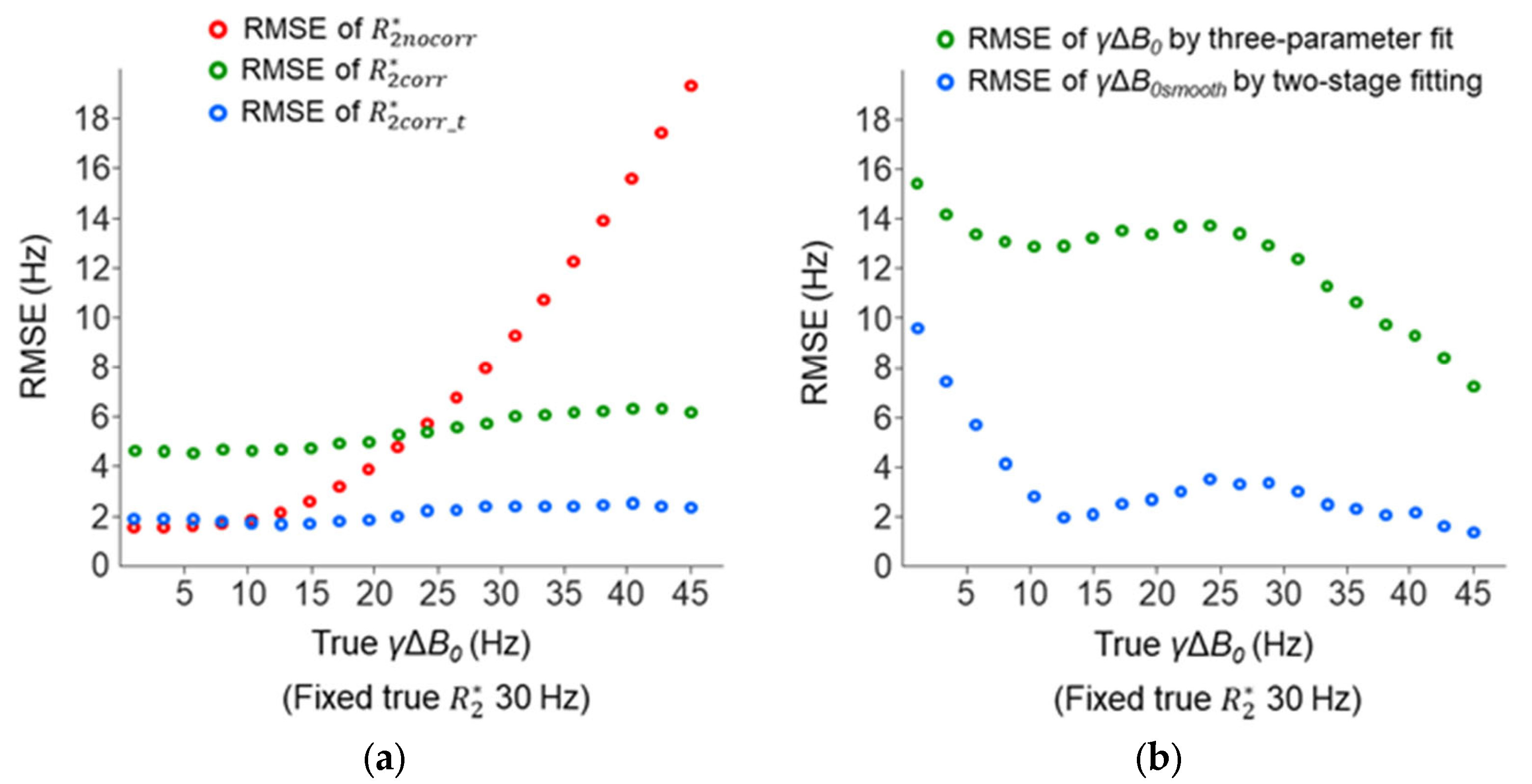
Further simulations were performed to study the accuracies of the
and
γΔ
B0 measurements with a varied cross-slice Δ
B0 effect (true γΔ
B0 increased from 1 to 45 Hz). The
became inaccurate with an increasing Δ
B0 effect (RMSE change: 1.6–19.3 Hz), whereas the accuracies of
and
were more consistent (RMSE changes: 4.6–6.4 Hz and 1.7–2.6 Hz) (
Figure 11a). The
was more accurate than
and was nearly as accurate as
when the Δ
B0 effect was small (true
γΔ
B0 < 10 Hz). The
γΔ
B0smooth measured by the two-stage fitting procedure was more accurate than the
γΔ
B0 measured by the three-parameter fit (
Figure 11b). The accuracy of the
γΔ
B0smooth decreased when the Δ
B0 effect was small (true
γΔ
B0 < 10 Hz), but this had little impact on the accuracy of
.
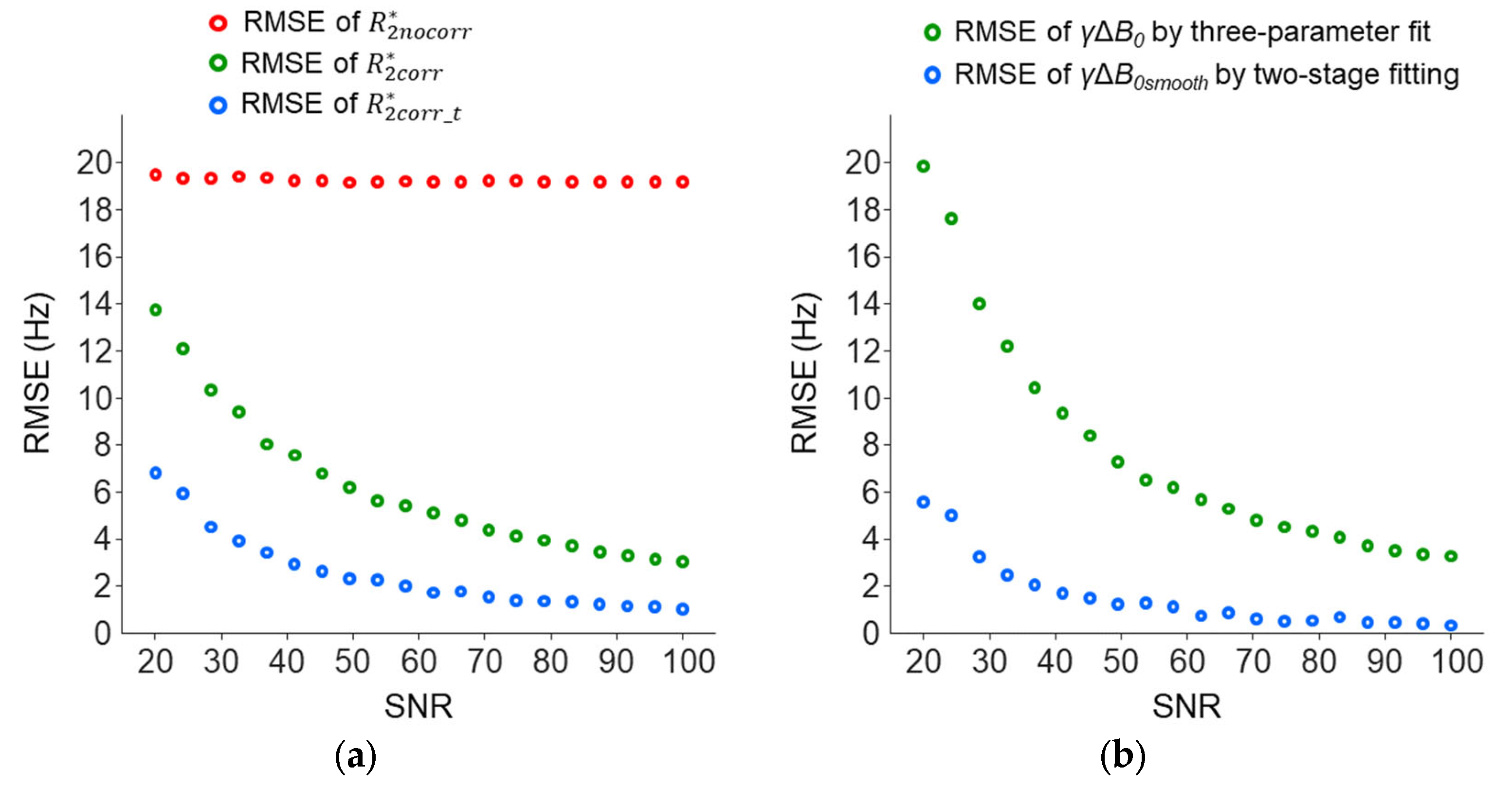
Simulations were also performed to study the dependence of the accuracies of the
and
γΔ
B0 measurements on the SNR. With a true
γΔ
B0 set to 45 Hz, the RMSE of the
was mainly contributed by the cross-slice Δ
B0 effect and showed a smaller dependence on the SNR levels; RMSE change: 19.3–19.7 Hz versus 3.2–14.1 Hz for
and 1.1–6.9 for
(
Figure 12a). Across the SNR levels,
was more accurate than
and
. The
γΔ
B0smooth measured using the two-stage fitting procedure was more accurate than the
γΔ
B0 measured using the three-parameter fit (
Figure 12b).
4. Discussion
The ΔB0 effects include a deviation of the GRE signal decay from the monoexponential model, a potential overestimate of the , and increased inter-subject SD of . With imaging data from eight mouse brains, we have shown that these ΔB0 effects were effectively mitigated using the three-parameter model in the selected ROIs. We have further demonstrated that the noise-related within-ROI SD of was significantly reduced by up to 30.2% using the two-stage fitting procedure. Moreover, simulations of measurements in the presence of a cross-slice ΔB0 effect and noise have demonstrated that was more accurate than . Taken together, these results support the use of the two-stage fitting procedure to mitigate ΔB0 effects and reduce noise sensitivity for measurement in the mouse brain.
Applying a smoothing filter to the
γΔ
B0 map for the two-stage fitting procedure assumes that the Δ
B0 is slowly varying on the x-y plane. Based on our results, this assumption may be valid in the selected corpus callosum, internal capsule, caudo-putamen, thalamus, and lateral ventricle regions of the mouse brain, where the application of the two-stage fitting procedure yields a significant reduction in the within-ROI SD of
by 7.7 to 30.2%. For the selected ROIs in the deep brain structure, including the internal capsule, caudo-putamen, and thalamus regions, the within-ROI SD of the
in these ROIs was further reduced with a larger smoothing kernel applied to the
γΔ
B0 map. However, the assumption of a slow in-plane variation in
γΔ
B0 is invalid in regions with a rapidly varying
γΔ
B0 on the x-y plane, such as the somatosensory cortex region close to air–tissue interfaces and with large magnetic susceptibility changes. In these regions, the
γΔ
B0 map as well as
showed a strong dependence on the smoothing kernel. Furthermore, the application of a larger smoothing kernel only led to small changes (<2%) in the within-ROI SD of
, indicating no benefits of using a larger smoothing kernel in these regions. In the presence of a fast in-plane variation in
γΔ
B0, applying a smoothing filter may lead to an underestimate of
γΔ
B0 and an overestimate of
[
17]. This
change may in turn increase the within-ROI SD of
and offset the benefit of the two-stage fitting procedure to reduce noise sensitivity. Considering the tradeoff, this study used a smoothing kernel of 390 µm, around 2.5 times the in-plane image resolution, for the two-stage fitting procedure. Importantly, we observed only a moderate dependence of the mean
on the smoothing kernel in the selected ROIs; the changes were less than 11.4%.
In our study, the
γΔ
B0 map was measured through the fitting of the six echo magnitude images with the three-parameter model that assumes a linear Δ
B0 across a slice. The assumption of a linear Δ
B0 implies a slowly varying Δ
B0 across a slice and may be invalid in regions with a rapidly varying cross-slice Δ
B0, such as a high Δ
B0. In our study, regions with a measured
γΔ
B0 larger than 60 Hz, such as the olfactory bulb, entorhinal cortex, and cerebellum, showed a potential overestimate of the
and thus an inaccurate estimate of the
γΔ
B0 map using the three-parameter model (
Figure 2). An alternative approach to measuring the
γΔ
B0 map is using phase images [
19,
20,
21,
22]. The phase image-based approach typically requires phase unwrapping procedures and an assumption of a smoothed
B0 on the x-y plane to reliably measure the
B0 map. Thus, the phase-based approach remains limited in the presence of a rapidly varying Δ
B0 across a slice or at high fields with a fast phase evolution. Our study demonstrates the feasibility of measuring the
γΔ
B0 map through the fitting to magnitude images, omitting the need for processing the phase images.
The use of magnitude images to measure the γΔB0 map relies on the sinc function-weighted signal decay, which is particularly pronounced at long echo times. When the ΔB0 effect is small, e.g., γΔB0 < 10 Hz, the signal attenuation may be too small to reliably measure the γΔB0. As shown in our simulation, the accuracy of the γΔB0smooth decreased when the true γΔB0 was less than 10 Hz. However, the inaccurate γΔB0smooth had little impact on the accuracy of the in our simulation. When the ΔB0 effect is small, the ΔB0 effect on the signal attenuation may be indifferentiable from the noise, and the accuracy of the γΔB0smooth becomes less relevant to the . On the other hand, phase-based methods may be more sensitive to detecting ΔB0-induced phase changes even when the ΔB0 effect is small. This may lead to more accurate estimates of γΔB0 and .
In addition to the increased within-ROI SD of the
measurement, a low SNR could induce bias in
measurement. In regions with a rapidly varying cross-slice Δ
B0, the sinc function-weighted signal decay is faster than the monoexponential decay at longer echo times, resulting in low SNR. In our study, the average SNR of the mouse brain’s 1st echo image (TE = 2.5 ms) was around 50. Given a
of 30 Hz and the measured
γΔ
B0 of 10–50 Hz in our selected ROIs, the SNR of the longest echo signal (TE = 22.5 ms) is around 15–27. However, the SNR at TE = 22.5 ms drops to 3–11 when the
γΔ
B0 is increased to 60–80 Hz in the olfactory bulb, entorhinal cortex, and cerebellum regions. This
γΔ
B0-induced signal drop at longer echo times may affect the ability of the three-parameter model to characterize the signal decay, likely resulting in an underestimate of
γΔ
B0 and an overestimate of
[
17].
The presented two-stage fitting procedure is based on the three-parameter model; therefore, it remains subject to the limitations of the three-parameter model in the presence of a rapidly varying cross-slice Δ
B0 as described above. Considering these limitations, this study focused on the ROIs with a
γΔ
B0 less than 50 Hz. To account for a rapidly varying cross-slice Δ
B0, previous studies have used separate data acquisition for a 3D high-resolution
γΔ
B0 map [
16,
18] and a quadratic function to approximate the cross-slice Δ
B0 [
16]. However, such approaches increase the scan time and require more fitting parameters to mitigate the Δ
B0 effect.
Our method shares some similarities with previous works by Dong et al. [
34] and Tan et al. [
35] in seeking the optimized solution for multiple parametric measurements that ensures data consistency and the smoothness of the phase maps. The major difference is that the previous works include the regularization of the loss function to ensure the smoothness of the phase maps, allowing one to address the optimization with more unknowns and more constraints. In contrast, our method ensures data consistency through the voxel-wise fitting, followed by applying a smoothing filter to smooth the phase maps. Solving regularized optimization normally requires multiple iterations and a longer computation time. Our method requires a short computation time but is limited to addressing a simple problem. Another difference is that the work by Tan et al. [
35] involves joint image reconstruction and parametric measurements for optimization. This allows one to reconstruct the undersampled k-space data with potential benefits in shortening the scan time and reducing motion artifacts. By contrast, our method only performs parametric measurements on the magnitude images, which are reconstructed using a vendor-supplied image reconstruction routine. Therefore, our method does not require k-space data and can be generally applied to multi-echo GRE images retrospectively.
In this study, multi-echo GRE acquisition was performed using the axial orientation with 18 slices to cover the entire brain. Another common option for 2D acquisition is to use the coronal orientation. However, the axial orientation allows one to cover a larger area of the mouse brain in a 2D slice than the coronal orientation. This is beneficial to our proposed method due to a smaller proportion of an axial image being influenced by large magnetic susceptibility changes near the aural cavity or air–tissue interfaces. Therefore, the assumption of a slow in-plane variation in γΔB0 can be applicable to a larger region of the brain, allowing the smoothing filter to effectively reduce the noise effect on the γΔB0 map.
This study applied and AIC to evaluate the goodness-of-fit. For each image voxel, the was used to determine whether the individual model fits the data considering the noise and the degrees of freedom of the model. Following the exclusion of the image voxels with a poor fit, AIC was applied subsequently to compare the goodness-of-fit of the models within each ROI considering the complexity of the model. Either assessment can eliminate the possibility of over-fitting. Therefore, this study focused on whether the application of the three-parameter model or two-stage fitting procedure improves the monoexponential fit rather than finding the best model to fit the data.
