
FOX Optimization Algorithm Based on Adaptive Spiral Flight and Multi-Strategy Fusion


Abstract
1. Introduction
2. Fox Optimization Algorithm
3. FOX Optimization Algorithm for Adaptive Spiral Flight
3.1. Tent Chaotic Mapping Based on Random Variables
3.2. Adaptive Inertia Weight
3.3. Levy Flight Mechanism
3.4. Variable Spiral Search Strategy
3.5. Time Complexity Analysis
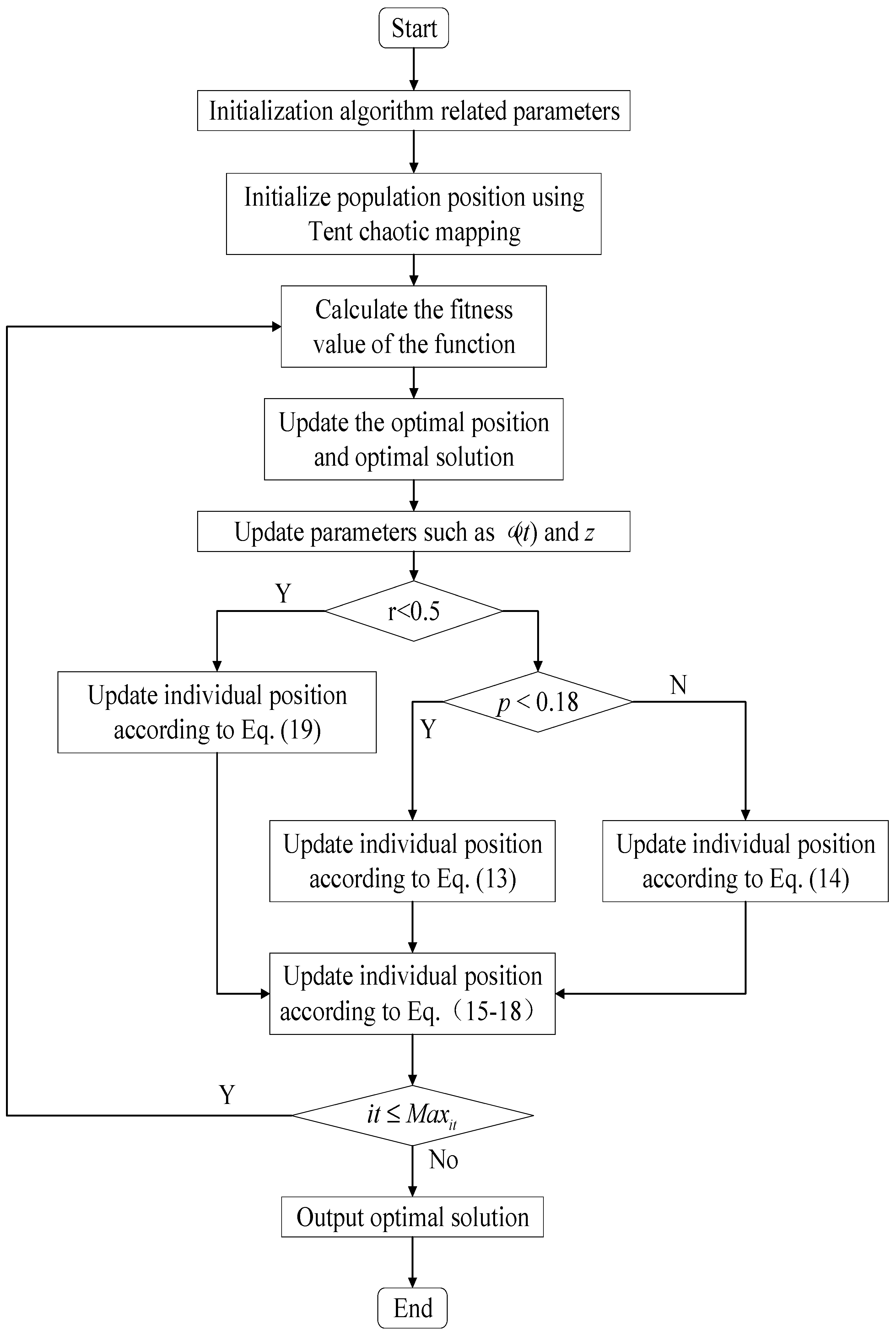
3.6. Algorithm Flowchart and Pseudocode
| Algorithm 1 Pseudo code of ASFFOX algorithm |
| 1: Initialize the population according to Equation (11); 2: While it < Maxit 3: Initialize Dist_S_T,Sp_S,Time_S_T,BestX,Dist_Fox_Prey,Jump,MinT,a,BestFitness,ω(t); 4: Calculate the fitness of each search agent 5: Select BestX and BestFitness among the population(X) in each iteration; 6: If1 fitness(Xit) > fitness(Xit+1) 7: BestFitness = fitness(Xit+1); 8: BestX = X(i,:); 9: Endif1 10: If2 r ≥ 0.5 11: If3 p > 0.18 12: Initialize time randomly; 13: Calculate Distance_Sound_travels using Equation (1); 14: Calculate Sp_S from Equation (2); 15: Calculate distance from fox to prey using Equation (3); 16: Tt = average time; 17: T = Tt/2; 18: Calculate jump using Equation (4) 19: Find Xit+1 using Equation (13); 20: Elseif p ≤ 0.18 21: Initialize time randomly; 22: Calculate Distance_Sound_travels using Equation (1) 23: Calculate Sp_S from Equation (2) 24: Calculate distance from fox to prey using Equation (3) 25: Tt = average time; 26: T = Tt/2; 27: Calculate jump using Equation (4) 28: Find Xit+1 using Equation (14); 29: EndIf3 30: else 31: Find MinT using Equation (7); 32: Explore Xit+1 using Equations (19) and (20); 33: EndIf2 34: Explore Xit+1 using Equations (15)–(18); 35: Check and amend the position if it goes beyond the limits; 36: Evaluate search agents by their fitness; 37: Update BestX; 38: it = it + 1; 39: End while 40: return BestX and BestFitness |
4. Simulation Experiment Results and Analysis
4.1. Experimental Parameter Settings
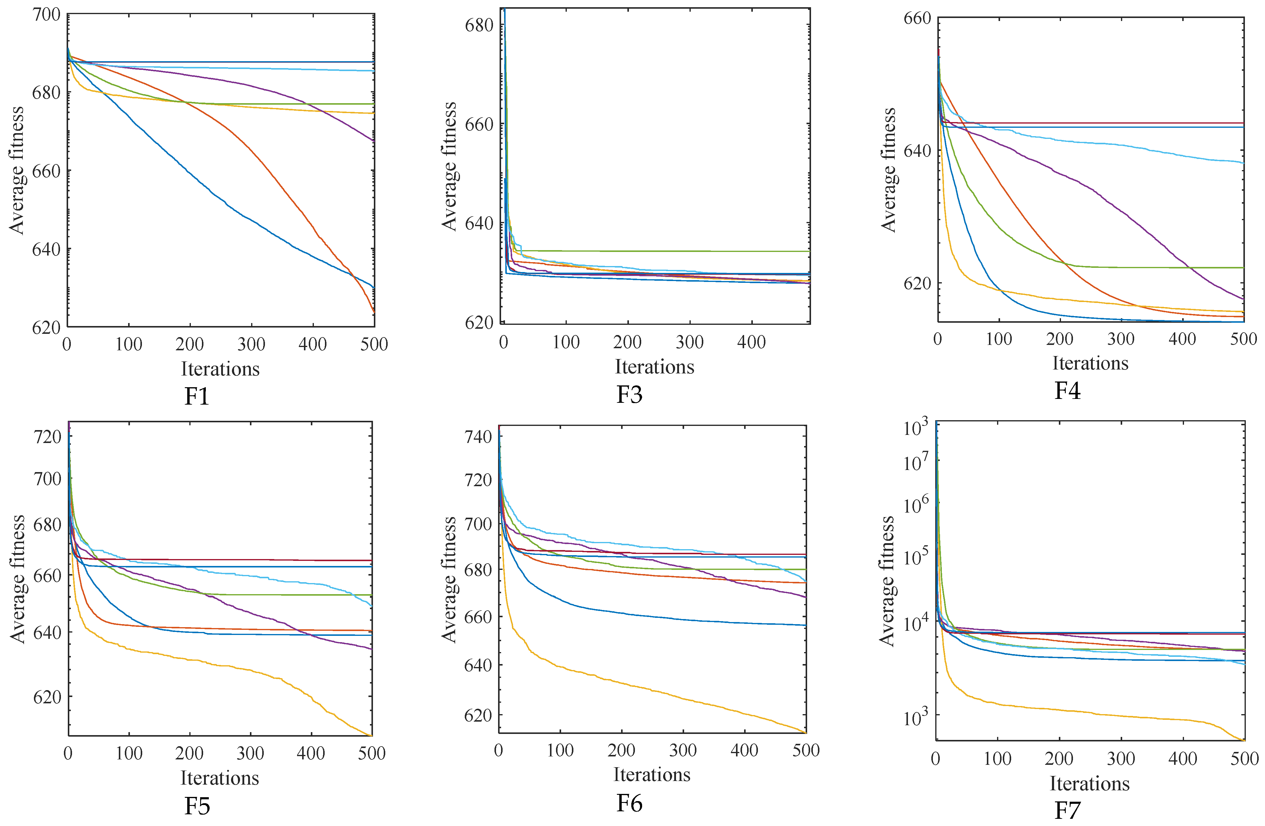
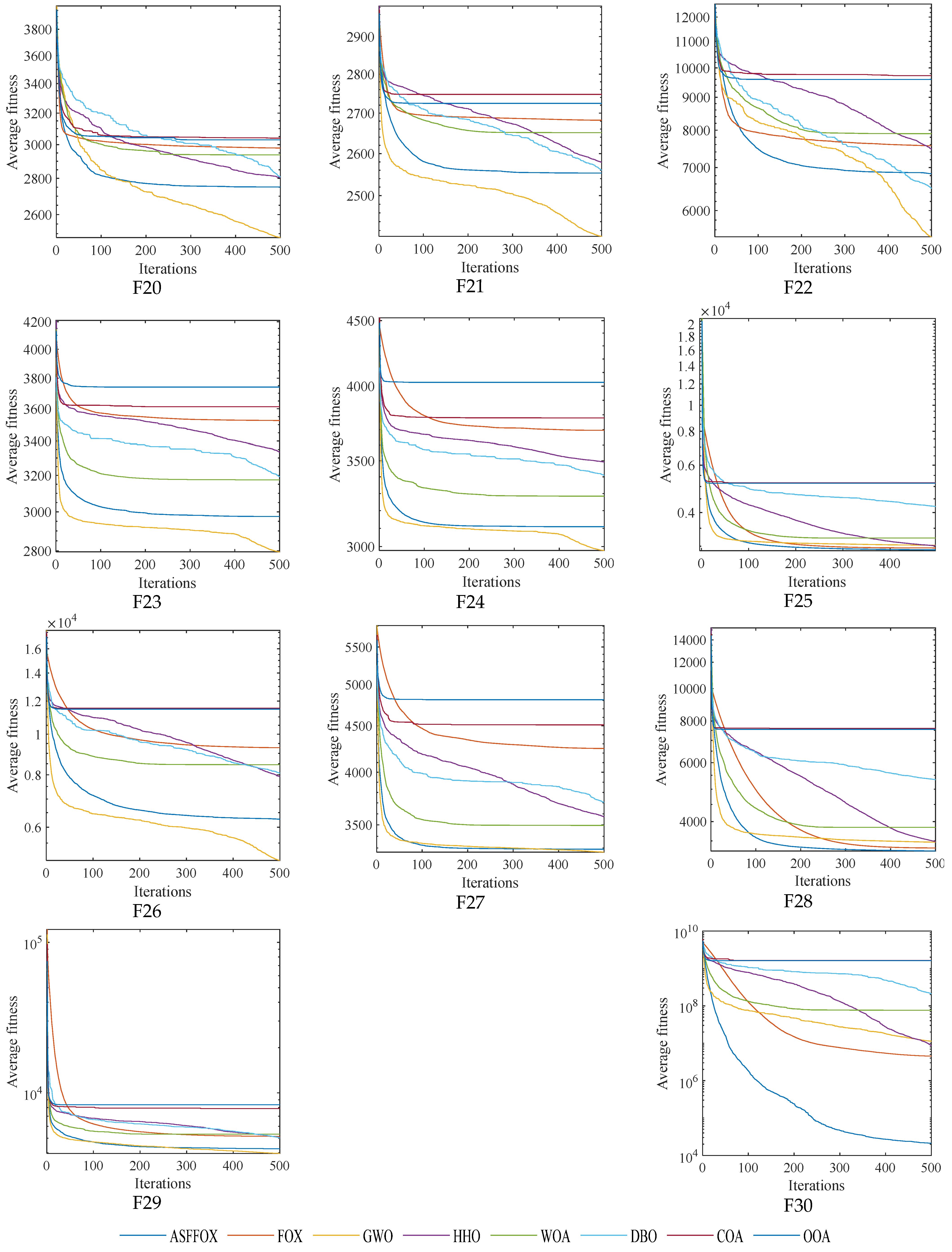
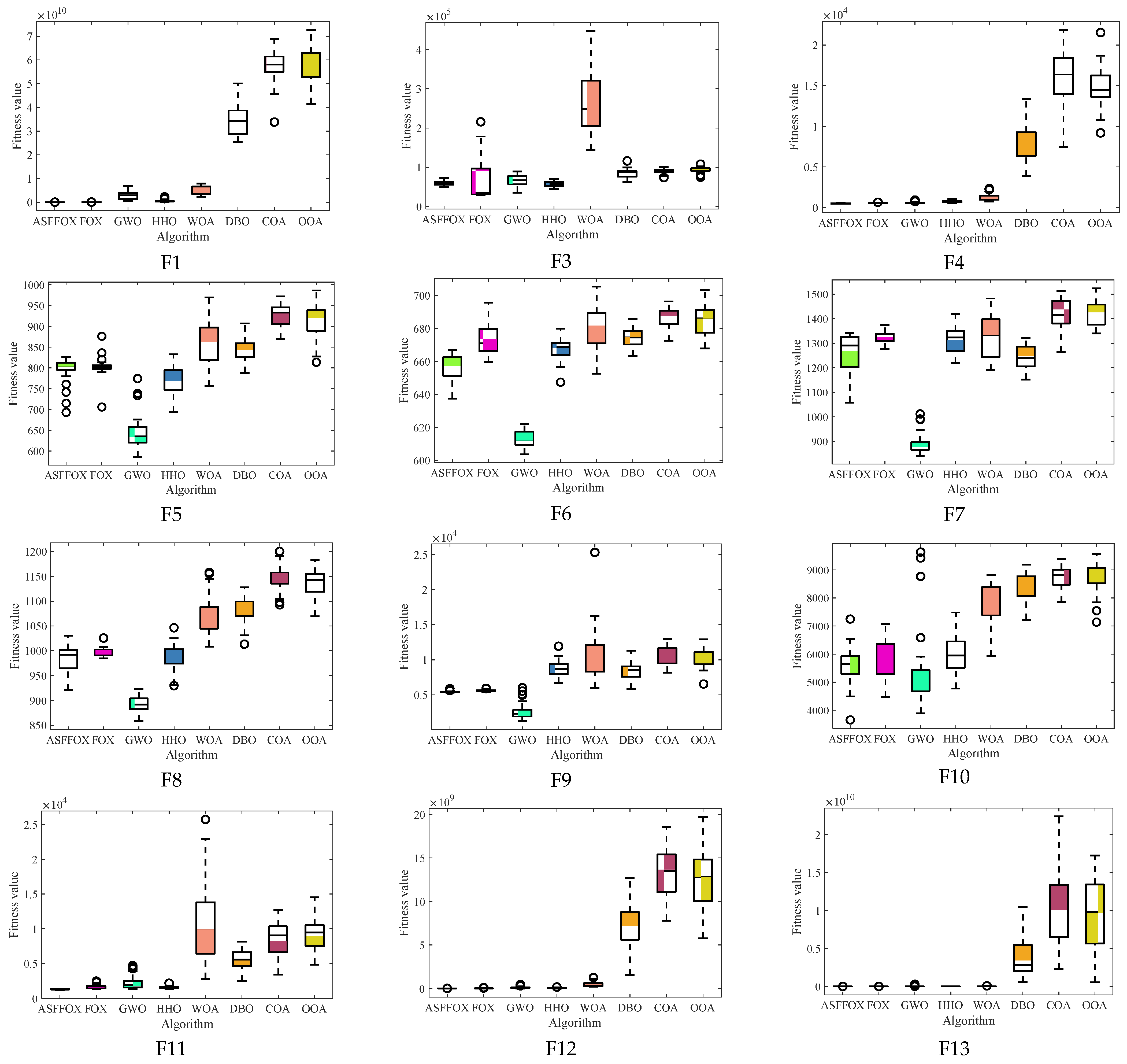
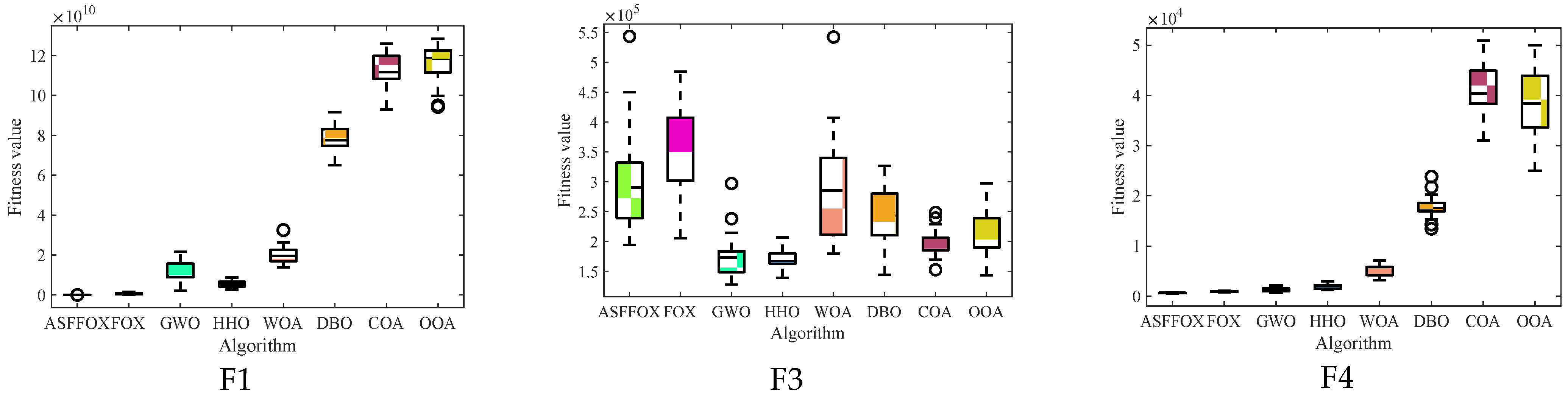
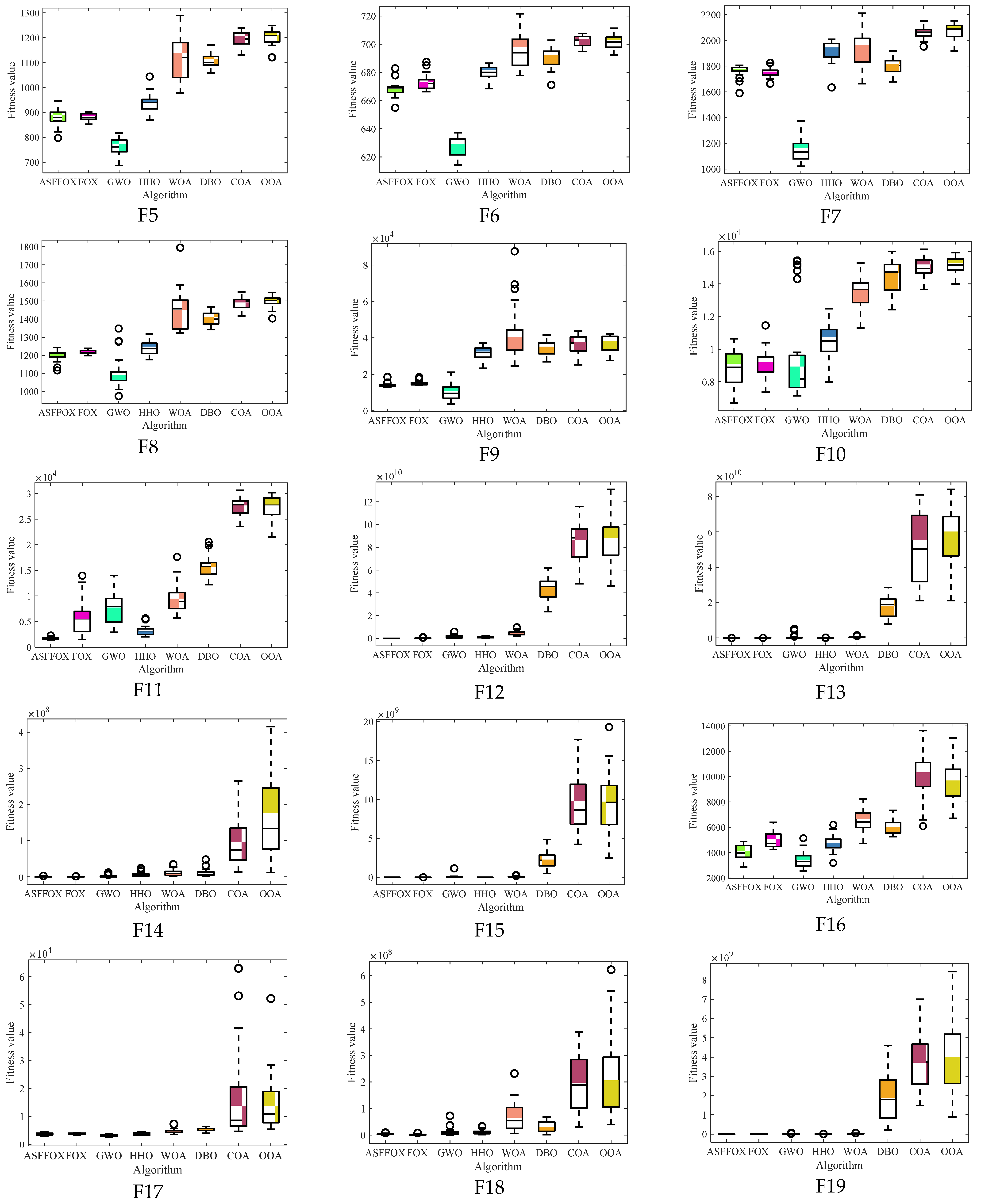
4.2. Comparative Analysis of ASFFOX and Other Metaheuristic Algorithms
4.3. High Dimensional Benchmark Function Testing
4.4. Wilcoxon Rank Sum Test
4.5. Application of Engineering Optimization Problems
4.5.1. Optimization Problem of I-Beam Design
4.5.2. Weight Minimization of a Speed Reducer
5. Conclusions
Author Contributions
Funding
Data Availability Statement
Conflicts of Interest
References
- Yue, Y.; Cao, L.; Lu, D.; Hu, Z.; Xu, M.; Wang, S.; Li, B.; Ding, H. Review and empirical analysis of sparrow search algorithm. Artif. Intell. Rev. 2023, 56, 10867–10919. [Google Scholar] [CrossRef]
- Wang, S.; Cao, L.; Chen, Y.; Chen, C.; Yue, Y.; Zhu, W. Gorilla optimization algorithm combining sine cosine and cauchy variations and its engineering applications. Sci. Rep. 2024, 14, 7578. [Google Scholar] [CrossRef] [PubMed]
- Yue, Y.; Cao, L.; Zhang, Y. Novel WSN Coverage Optimization Strategy Via Monarch Butterfly Algorithm and Particle Swarm Optimization. Wirel. Pers. Commun. 2024, 135, 2255–2280. [Google Scholar] [CrossRef]
- Yue, Y.; You, H.; Wang, S.; Cao, L. Improved whale optimization algorithm and its application in heterogeneous wireless sensor networks. Int. J. Distrib. Sens. Netw. 2021, 17, 15501477211018140. [Google Scholar] [CrossRef]
- Chen, C.; Cao, L.; Chen, Y.; Chen, B.; Yue, Y. A comprehensive survey of convergence analysis of beetle antennae search algorithm and its applications. Artif. Intell. Rev. 2024, 57, 141. [Google Scholar] [CrossRef]
- Cao, L.; Chen, H.; Chen, Y.; Yue, Y.; Zhang, X. Bio-Inspired Swarm Intelligence Optimization Algorithm-Aided Hybrid TDOA/AOA-Based Localization. Biomimetics 2023, 8, 186. [Google Scholar] [CrossRef]
- Yue, Y.; Cao, L.; Chen, H.; Chen, Y.; Su, Z. Towards an Optimal KELM Using the PSO-BOA Optimization Strategy with Applications in Data Classification. Biomimetics 2023, 8, 306. [Google Scholar] [CrossRef]
- Chen, B.; Cao, L.; Chen, C.; Chen, Y.; Yue, Y. A comprehensive survey on the chicken swarm optimization algorithm and its applications: State-of-the-art and research challenges. Artif. Intell. Rev. 2024, 57, 170. [Google Scholar] [CrossRef]
- Kennedy, J.; Eberhart, R. Particle swarm optimization. In Proceedings of the ICNN’95-International Conference on Neural Networks, Perth, WA, Australia, 27 November 1995; IEEE: Piscataway, NJ, USA, 1995; Volume 4, pp. 1942–1948. [Google Scholar]
- Abdollahzadeh, B.; Soleimanian Gharehchopogh, F.; Mirjalili, S. Artificial gorilla troops optimizer: A new nature-inspired metaheuristic algorithm for global optimization problems. Int. J. Intell. Syst. 2021, 36, 5887–5958. [Google Scholar] [CrossRef]
- Dhiman, G.; Kumar, V. Seagull optimization algorithm: Theory and its applications for large-scale industrial engineering problems. Knowl.-Based Syst. 2019, 165, 169–196. [Google Scholar] [CrossRef]
- Xue, J.; Shen, B. A novel swarm intelligence optimization approach: Sparrow search algorithm. Syst. Sci. Control Eng. 2020, 8, 22–34. [Google Scholar] [CrossRef]
- Zhao, S.; Zhang, T.; Ma, S.; Chen, M. Dandelion Optimizer: A nature-inspired metaheuristic algorithm for engineering applications. Eng. Appl. Artif. Intell. 2022, 114, 105075. [Google Scholar] [CrossRef]
- Nadimi-Shahraki, M.H.; Zamani, H.; Asghari Varzaneh, Z. A systematic review of the whale optimization algorithm: Theoretical foundation, improvements, and hybridizations. Arch. Comput. Methods Eng. 2023, 30, 4113–4159. [Google Scholar] [CrossRef]
- Chopra, N.; Ansari, M.M. Golden jackal optimization: A novel nature-inspired optimizer for engineering applications. Expert Syst. Appl. 2022, 198, 116924. [Google Scholar] [CrossRef]
- Mohammed, H.; Rashid, T. FOX: A FOX-inspired optimization algorithm. Appl. Intell. 2023, 53, 1030–1050. [Google Scholar] [CrossRef]
- Hu, G.; Song, K.; Li, X. DEMFFA: A multi-strategy modified Fennec Fox algorithm with mixed improved differential evolutionary variation strategies. J. Big Data 2024, 11, 69. [Google Scholar] [CrossRef]
- Fu, Z.; An, J.; Yang, Q.; Yuan, H.; Sun, Y.; Ebrahimian, H. Skin cancer detection using kernel fuzzy C-means and developed red fox optimization algorithm. Biomed. Signal Process. Control 2022, 71, 103160. [Google Scholar] [CrossRef]
- Zhang, C.; Liu, L.; Yang, Y.; Yu, S.; Ning, J.; Zhang, Y.; Zhang, C.; Guo, Y. An Opposition-Based Learning-Based Search Mechanism for Flying Foxes Optimization Algorithm. Comput. Mater. Contin. 2024, 79, 5201–5223. [Google Scholar] [CrossRef]
- Natarajan, R.; Megharaj, G.; Marchewka, A.; Divakarachari, P.B.; Hans, M.R. Energy and distance based multi-objective red fox optimization algorithm in wireless sensor network. Sensors 2022, 22, 3761. [Google Scholar] [CrossRef]
- Pugal Priya, R.; Saradadevi Sivarani, T.; Gnana Saravanan, A. Deep long and short term memory based Red Fox optimization algorithm for diabetic retinopathy detection and classification. Int. J. Numer. Methods Biomed. Eng. 2022, 38, e3560. [Google Scholar] [CrossRef]
- Khorami, E.; Mahdi Babaei, F.; Azadeh, A. Optimal diagnosis of COVID-19 based on convolutional neural network and red fox optimization algorithm. Comput. Intell. Neurosci. 2021, 2021, 4454507. [Google Scholar] [CrossRef] [PubMed]
- Zhang, M.; Xu, Z.; Lu, X.; Liu, Y.; Xiao, Q.; Taheri, B. An optimal model identification for solid oxide fuel cell based on extreme learning machines optimized by improved Red Fox Optimization algorithm. Int. J. Hydrog. Energy 2021, 46, 28270–28281. [Google Scholar] [CrossRef]
- Xu, L.; Mohammadi, M. Brain tumor diagnosis from MRI based on Mobilenetv2 optimized by contracted fox optimization algorithm. Heliyon 2024, 10, E23866. [Google Scholar] [CrossRef] [PubMed]
- Huo, Z.; Liu, S.; Ebrahimian, H. Aircraft energy management system using chaos red fox optimization algorithm. J. Electr. Eng. Technol. 2022, 17, 179–195. [Google Scholar] [CrossRef]
- Zaborski, M.; Woźniak, M.; Mańdziuk, J. Multidimensional Red Fox meta-heuristic for complex optimization. Appl. Soft Comput. 2022, 131, 109774. [Google Scholar] [CrossRef]
- Zade, B.M.H.; Mansouri, N. Improved red fox optimizer with fuzzy theory and game theory for task scheduling in cloud environment. J. Comput. Sci. 2022, 63, 101805. [Google Scholar] [CrossRef]
- Zervoudakis, K.; Tsafarakis, S. A global optimizer inspired from the survival strategies of flying foxes. Eng. Comput. 2023, 39, 1583–1616. [Google Scholar] [CrossRef]
- Feda, A.K.; Adegboye, M.; Adegboye, O.R.; Agyekum, E.B.; Mbasso, W.F.; Kamel, S. S-shaped grey wolf optimizer-based FOX algorithm for feature selection. Heliyon 2024, 10, E24192. [Google Scholar] [CrossRef]
- Deepanraj, B.; Gugulothu, S.K.; Ramaraj, R.; Arthi, M.; Saravanan, R. Optimal parameter estimation of proton exchange membrane fuel cell using improved red fox optimizer for sustainable energy management. J. Clean. Prod. 2022, 369, 133385. [Google Scholar] [CrossRef]
- Černý, R.; Favre-Nicolin, V.; Rohlíček, J.; Hušák, M. FOX, current state and possibilities. Crystals 2017, 7, 322. [Google Scholar] [CrossRef]
- Sharma, R.; Mahanti, G.K.; Panda, G.; Rath, A.; Dash, S.; Mallik, S.; Zhao, Z. Comparative performance analysis of binary variants of FOX optimization algorithm with half-quadratic ensemble ranking method for thyroid cancer detection. Sci. Rep. 2023, 13, 19598. [Google Scholar] [CrossRef] [PubMed]
- Zhang, C.; Song, Z.; Yang, Y.; Zhang, C.; Guo, Y. A Decomposition-Based Multi-Objective Flying Foxes Optimization Algorithm and Its Applications. Biomimetics 2024, 9, 417. [Google Scholar] [CrossRef] [PubMed]
- Vaiyapuri, T.; Liyakathunisa Alaskar, H.; Aljohani, E.; Shridevi, S.; Hussain, A. Red fox optimizer with data-science-enabled microarray gene expression classification model. Appl. Sci. 2022, 12, 4172. [Google Scholar] [CrossRef]
- Al-Daraiseh, A.; Sanjalawe, Y.; Al-E’mari, S.; Fraihat, S.; Bany Taha, M.; Al-Muhammed, M. Cryptographic Grade Chaotic Random Number Generator Based on Tent-Map. J. Sens. Actuator Netw. 2023, 12, 73. [Google Scholar] [CrossRef]
- Wang, Y.; Zhang, X.; Yu, D.J.; Bai, Y.J.; Du, J.P.; Tian, Z.T. Tent Chaotic Map and Population Classification Evolution Strategy-Based Dragonfly Algorithm for Global Optimization. Math. Probl. Eng. 2022, 2022, 2508414. [Google Scholar] [CrossRef]
- Cao, D.; Xu, Y.; Yang, Z.; Dong, H.; Li, X. An enhanced whale optimization algorithm with improved dynamic opposite learning and adaptive inertia weight strategy. Complex Intell. Syst. 2023, 9, 767–795. [Google Scholar] [CrossRef]
- Jena, J.J.; Satapathy, S.C. A new adaptive tuned Social Group Optimization (SGO) algorithm with sigmoid-adaptive inertia weight for solving engineering design problems. Multimed. Tools Appl. 2024, 83, 3021–3055. [Google Scholar] [CrossRef]
- Asif, M.; Nagra, A.A.; Ahmad, M.B.; Masood, K. Feature selection empowered by self-inertia weight adaptive particle swarm optimization for text classification. Appl. Artif. Intell. 2022, 36, 2004345. [Google Scholar] [CrossRef]
- Bakir, H.; Guvenc, U.; Kahraman, H.T.; Duman, S. Improved Lévy flight distribution algorithm with FDB-based guiding mechanism for AVR system optimal design. Comput. Ind. Eng. 2022, 168, 108032. [Google Scholar] [CrossRef]
- Kaidi, W.; Khishe, M.; Mohammadi, M. Dynamic levy flight chimp optimization. Knowl.-Based Syst. 2022, 235, 107625. [Google Scholar] [CrossRef]
- Geng, J.; Sun, X.; Wang, H.; Bu, X.; Liu, D.; Li, F.; Zhao, Z. A modified adaptive sparrow search algorithm based on chaotic reverse learning and spiral search for global optimization. Neural Comput. Appl. 2023, 35, 24603–24620. [Google Scholar] [CrossRef]
- Li, M.; Xu, G.; Fu, Y.; Zhang, T.; Du, L. Improved whale optimization algorithm based on variable spiral position update strategy and adaptive inertia weight. J. Intell. Fuzzy Syst. 2022, 42, 1501–1517. [Google Scholar] [CrossRef]
- Wang, W.; Chen, Y.; Yang, C.; Li, Y.; Xu, B.; Huang, K.; Xiang, C. An efficient optimal sizing strategy for a hybrid electric air-ground vehicle using adaptive spiral optimization algorithm. J. Power Sources 2022, 517, 230704. [Google Scholar] [CrossRef]
- Li, Y.; Lin, X.; Liu, J. An improved gray wolf optimization algorithm to solve engineering problems. Sustainability 2021, 13, 3208. [Google Scholar] [CrossRef]
- Heidari, A.A.; Mirjalili, S.; Faris, H.; Aljarah, I.; Mafarja, M.; Chen, H. Harris hawks optimization: Algorithm and applications. Future Gener. Comput. Syst. 2019, 97, 849–872. [Google Scholar] [CrossRef]
- Mirjalili, S.; Lewis, A. The whale optimization algorithm. Adv. Eng. Softw. 2016, 95, 51–67. [Google Scholar] [CrossRef]
- Xue, J.; Shen, B. Dung beetle optimizer: A new meta-heuristic algorithm for global optimization. J. Supercomput. 2023, 79, 7305–7336. [Google Scholar] [CrossRef]
- Jia, H.; Rao, H.; Wen, C.; Mirjalili, S. Crayfish optimization algorithm. Artif. Intell. Rev. 2023, 56, 1919–1979. [Google Scholar] [CrossRef]
- Dehghani, M.; Trojovský, P. Osprey optimization algorithm: A new bio-inspired metaheuristic algorithm for solving engineering optimization problems. Front. Mech. Eng. 2023, 8, 1126450. [Google Scholar] [CrossRef]
- Wang, L.; Zhu, M.; Yue, W.; Dong, J. Experimental and topology optimization design study of the shear behaviour of reinforced concrete I-beam web with opening. Eng. Optim. 2022, 54, 1509–1524. [Google Scholar] [CrossRef]
- Xin, W.; Zhang, Y.; Fu, Y.; Yang, W.; Zheng, H. A multi-objective optimization design approach of large mining planetary gear reducer. Sci. Rep. 2023, 13, 18640. [Google Scholar] [CrossRef] [PubMed]


| No. | Functions | Fi = Fi(x) | |
|---|---|---|---|
| Unimodal Functions | 1 | Shifted and Rotated Bent Cigar Function | 100 |
| 2 | Shifted and Rotated Sum of Different Power Function * | 200 | |
| 3 | Shifted and Rotated Zakharov Function | 300 | |
| Simple Multimodal Functions | 4 | Shifted and Rotated Rosenbrock’s Function | 400 |
| 5 | Shifted and Rotated Rastrigin’s Function | 500 | |
| 6 | Shifted and Rotated Expanded Scaffer’s F6 Function | 600 | |
| 7 | Shifted and Rotated Lunacek Bi_Rastrigin Function | 700 | |
| 8 | Shifted and Rotated Non-Continuous Rastrigin’s Function | 800 | |
| 9 | Shifted and Rotated Levy Function | 900 | |
| 10 | Shifted and Rotated Schwefel’s Function | 1000 | |
| Hybrid Functions | 11 | Hybrid Function 1 (N = 3) | 1100 |
| 12 | Hybrid Function 2 (N = 3) | 1200 | |
| 13 | Hybrid Function 3 (N = 3) | 1300 | |
| 14 | Hybrid Function 4 (N = 4) | 1400 | |
| 15 | Hybrid Function 5 (N = 4) | 1500 | |
| 16 | Hybrid Function 6 (N = 4) | 1600 | |
| 17 | Hybrid Function 6 (N = 5) | 1700 | |
| 18 | Hybrid Function 6 (N = 5) | 1800 | |
| 19 | Hybrid Function 6 (N = 5) | 1900 | |
| 20 | Hybrid Function 6 (N = 6) | 2000 | |
| Composition Functions | 21 | Composition Function 1 (N = 3) | 2100 |
| 22 | Composition Function 2 (N = 3) | 2200 | |
| 23 | Composition Function 3 (N = 4) | 2300 | |
| 24 | Composition Function 4 (N = 4) | 2400 | |
| 25 | Composition Function 5 (N = 5) | 2500 | |
| 26 | Composition Function 6 (N = 5) | 2600 | |
| 27 | Composition Function 7 (N = 6) | 2700 | |
| 28 | Composition Function 8 (N = 6) | 2800 | |
| 29 | Composition Function 9 (N = 3) | 2900 | |
| 30 | Composition Function 10 (N = 3) | 3000 | |
| Search Range: [−100, 100] | |||
| ASFFOX | FOX | GWO | HHO | WOA | DBO | COA | OOA | ||
|---|---|---|---|---|---|---|---|---|---|
| F1 | min | 1.52 × 10⁴ | 1.19 × 10⁴ | 3.53 × 10⁸ | 9.25 × 10⁷ | 2.26 × 10⁹ | 2.53 × 10¹⁰ | 3.38 × 10¹⁰ | 4.14 × 10¹⁰ |
| F1 | std | 7.55 × 10⁴ | 9.01 × 10³ | 1.64 × 10⁹ | 4.48 × 10⁸ | 1.65 × 10⁹ | 6.42 × 10⁹ | 6.76 × 10⁹ | 7.83 × 10⁹ |
| F1 | avg | 9.99 × 10⁴ | 2.32 × 10⁴ | 2.85 × 10⁹ | 5.34 × 10⁸ | 4.89 × 10⁹ | 3.43 × 10¹⁰ | 5.73 × 10¹⁰ | 5.82 × 10¹⁰ |
| F3 | min | 5.02 × 10⁴ | 2.79 × 10⁴ | 3.53 × 10⁴ | 4.39 × 10⁴ | 1.44 × 10⁵ | 6.17 × 10⁴ | 7.37 × 10⁴ | 7.44 × 10⁴ |
| F3 | std | 5.07 × 10³ | 5.37 × 10⁴ | 1.31 × 10⁴ | 6.92 × 10³ | 6.91 × 10⁴ | 1.12 × 10⁴ | 6.25 × 10³ | 6.73 × 10³ |
| F3 | avg | 5.92 × 10⁴ | 6.70 × 10⁴ | 6.62 × 10⁴ | 5.77 × 10⁴ | 2.63 × 10⁵ | 8.56 × 10⁴ | 9.01 × 10⁴ | 9.30 × 10⁴ |
| F4 | min | 4.65 × 10² | 5.21 × 10² | 5.19 × 10² | 5.06 × 10² | 7.47 × 10² | 3.88 × 10³ | 7.45 × 10³ | 9.18 × 10³ |
| F4 | std | 2.44 × 101 | 3.14 × 101 | 8.17 × 101 | 1.41 × 10² | 4.08 × 10² | 2.23 × 10³ | 3.49 × 10³ | 2.53 × 10³ |
| F4 | avg | 5.08 × 10² | 5.58 × 10² | 6.09 × 10² | 7.55 × 10² | 1.30 × 10³ | 7.93 × 10³ | 1.60 × 10⁴ | 1.48 × 10⁴ |
| F5 | min | 6.93 × 10² | 7.06 × 10² | 5.86 × 10² | 6.94 × 10² | 7.57 × 10² | 7.88 × 10² | 8.69 × 10² | 8.14 × 10² |
| F5 | std | 3.14 × 101 | 2.43 × 101 | 4.18 × 101 | 3.27 × 101 | 6.59 × 101 | 2.64 × 101 | 2.94 × 101 | 4.08 × 101 |
| F5 | avg | 7.94 × 10² | 8.02 × 10² | 6.45 × 10² | 7.71 × 10² | 8.63 × 10² | 8.44 × 10² | 9.27 × 10² | 9.15 × 10² |
| F6 | min | 6.37 × 10² | 6.60 × 10² | 6.04 × 10² | 6.47 × 10² | 6.53 × 10² | 6.63 × 10² | 6.73 × 10² | 6.68 × 10² |
| F6 | std | 7.99 × 100 | 9.41 × 100 | 4.96 × 100 | 6.64 × 100 | 1.18 × 101 | 5.84 × 100 | 5.99 × 100 | 8.47 × 100 |
| F6 | avg | 6.56 × 10² | 6.74 × 10² | 6.13 × 10² | 6.68 × 10² | 6.80 × 10² | 6.75 × 10² | 6.86 × 10² | 6.85 × 10² |
| F7 | min | 1.06 × 10³ | 1.28 × 10³ | 8.42 × 10² | 1.22 × 10³ | 1.19 × 10³ | 1.15 × 10³ | 1.26 × 10³ | 1.34 × 10³ |
| F7 | std | 7.44 × 101 | 2.34 × 101 | 4.31 × 101 | 5.10 × 101 | 8.12 × 101 | 4.80 × 101 | 6.38 × 101 | 4.86 × 101 |
| F7 | avg | 1.26 × 10³ | 1.32 × 10³ | 8.94 × 10² | 1.32 × 10³ | 1.33 × 10³ | 1.24 × 10³ | 1.42 × 10³ | 1.43 × 10³ |
| F8 | min | 9.21 × 10² | 9.85 × 10² | 8.59 × 10² | 9.30 × 10² | 1.01 × 10³ | 1.01 × 10³ | 1.09 × 10³ | 1.07 × 10³ |
| F8 | std | 2.75 × 101 | 7.99 × 100 | 1.67 × 101 | 2.73 × 101 | 4.00 × 101 | 2.65 × 101 | 2.43 × 101 | 2.97 × 101 |
| F8 | avg | 9.84 × 10² | 9.99 × 10² | 8.92 × 10² | 9.88 × 10² | 1.07 × 10³ | 1.08 × 10³ | 1.14 × 10³ | 1.14 × 10³ |
| F9 | min | 5.32 × 10³ | 5.41 × 10³ | 1.25 × 10³ | 6.71 × 10³ | 5.99 × 10³ | 5.85 × 10³ | 8.18 × 10³ | 6.55 × 10³ |
| F9 | std | 1.09 × 10² | 1.40 × 10² | 1.26 × 10³ | 1.13 × 10³ | 3.77 × 10³ | 1.23 × 10³ | 1.39 × 10³ | 1.38 × 10³ |
| F9 | avg | 5.45 × 10³ | 5.62 × 10³ | 2.72 × 10³ | 8.76 × 10³ | 1.05 × 10⁴ | 8.52 × 10³ | 1.06 × 10⁴ | 1.03 × 10⁴ |
| F10 | min | 3.65 × 10³ | 4.47 × 10³ | 3.88 × 10³ | 4.77 × 10³ | 5.94 × 10³ | 7.22 × 10³ | 7.85 × 10³ | 7.14 × 10³ |
| F10 | std | 6.91 × 10² | 6.95 × 10² | 1.44 × 10³ | 6.40 × 10² | 6.62 × 10² | 5.03 × 10² | 4.12 × 10² | 5.49 × 10² |
| F10 | avg | 5.60 × 10³ | 5.79 × 10³ | 5.39 × 10³ | 6.01 × 10³ | 7.75 × 10³ | 8.42 × 10³ | 8.74 × 10³ | 8.71 × 10³ |
| F11 | min | 1.21 × 10³ | 1.28 × 10³ | 1.39 × 10³ | 1.36 × 10³ | 2.79 × 10³ | 2.48 × 10³ | 3.40 × 10³ | 4.83 × 10³ |
| F11 | std | 4.53 × 101 | 2.91 × 10² | 9.60 × 10² | 1.75 × 10² | 6.04 × 10³ | 1.40 × 10³ | 2.45 × 10³ | 2.47 × 10³ |
| F11 | avg | 1.29 × 10³ | 1.65 × 10³ | 2.27 × 10³ | 1.59 × 10³ | 1.12 × 10⁴ | 5.60 × 10³ | 8.68 × 10³ | 9.38 × 10³ |
| F12 | min | 2.56 × 10⁵ | 1.45 × 10⁶ | 7.85 × 10⁶ | 5.93 × 10⁶ | 2.17 × 10⁸ | 1.55 × 10⁹ | 7.80 × 10⁹ | 5.77 × 10⁹ |
| F12 | std | 1.66 × 10⁶ | 3.04 × 10⁷ | 1.02 × 10⁸ | 3.76 × 10⁷ | 2.71 × 10⁸ | 2.21 × 10⁹ | 2.83 × 10⁹ | 3.68 × 10⁹ |
| F12 | avg | 2.22 × 10⁶ | 2.32 × 10⁷ | 9.42 × 10⁷ | 5.82 × 10⁷ | 5.09 × 10⁸ | 7.16 × 10⁹ | 1.34 × 10¹⁰ | 1.27 × 10¹⁰ |
| F13 | min | 2.67 × 10³ | 2.00 × 10⁴ | 7.60 × 10⁴ | 5.06 × 10⁵ | 2.22 × 10⁶ | 5.78 × 10⁸ | 2.30 × 10⁹ | 5.49 × 10⁸ |
| F13 | std | 1.97 × 10⁴ | 7.41 × 10⁴ | 5.31 × 10⁷ | 2.99 × 10⁵ | 1.38 × 10⁷ | 2.54 × 10⁹ | 5.17 × 10⁹ | 4.99 × 10⁹ |
| F13 | avg | 1.94 × 10⁴ | 9.97 × 10⁴ | 1.75 × 10⁷ | 8.82 × 10⁵ | 1.28 × 10⁷ | 3.62 × 10⁹ | 1.04 × 10¹⁰ | 9.22 × 10⁹ |
| F14 | min | 1.07 × 10⁴ | 2.92 × 10³ | 8.09 × 10³ | 9.80 × 10⁴ | 6.07 × 10⁴ | 6.17 × 10⁴ | 4.60 × 10⁴ | 1.18 × 10⁵ |
| F14 | std | 1.08 × 10⁵ | 2.52 × 10⁵ | 1.06 × 10⁶ | 1.61 × 10⁶ | 2.92 × 10⁶ | 6.97 × 10⁵ | 2.17 × 10⁶ | 4.84 × 10⁶ |
| F14 | avg | 1.24 × 10⁵ | 2.06 × 10⁵ | 7.18 × 10⁵ | 1.47 × 10⁶ | 2.64 × 10⁶ | 9.72 × 10⁵ | 2.35 × 10⁶ | 4.49 × 10⁶ |
| F15 | min | 2.16 × 10³ | 7.01 × 10³ | 1.98 × 10⁴ | 4.10 × 10⁴ | 9.18 × 10⁴ | 3.77 × 10⁵ | 3.25 × 10⁷ | 1.99 × 10⁷ |
| F15 | std | 7.27 × 10³ | 2.62 × 10⁴ | 5.95 × 10⁶ | 7.83 × 10⁴ | 5.96 × 10⁶ | 1.35 × 10⁷ | 5.93 × 10⁸ | 4.30 × 10⁸ |
| F15 | avg | 8.28 × 10³ | 2.90 × 10⁴ | 2.22 × 10⁶ | 1.32 × 10⁵ | 4.52 × 10⁶ | 8.78 × 10⁶ | 6.86 × 10⁸ | 5.00 × 10⁸ |
| F16 | min | 2.29 × 10³ | 2.89 × 10³ | 2.11 × 10³ | 3.15 × 10³ | 2.96 × 10³ | 3.65 × 10³ | 4.17 × 10³ | 3.39 × 10³ |
| F16 | std | 3.67 × 10² | 5.77 × 10² | 4.24 × 10² | 3.33 × 10² | 5.73 × 10² | 2.63 × 10² | 1.01 × 10³ | 1.31 × 10³ |
| F16 | avg | 2.89 × 10³ | 3.86 × 10³ | 2.64 × 10³ | 3.66 × 10³ | 4.16 × 10³ | 4.04 × 10³ | 5.62 × 10³ | 6.12 × 10³ |
| F17 | min | 1.92 × 10³ | 2.22 × 10³ | 1.86 × 10³ | 2.24 × 10³ | 2.18 × 10³ | 2.39 × 10³ | 2.45 × 10³ | 2.93 × 10³ |
| F17 | std | 2.99 × 10² | 3.10 × 10² | 1.63 × 10² | 2.77 × 10² | 3.23 × 10² | 2.55 × 10² | 3.08 × 10³ | 4.11 × 10³ |
| F17 | avg | 2.59 × 10³ | 2.89 × 10³ | 2.11 × 10³ | 2.69 × 10³ | 2.76 × 10³ | 2.91 × 10³ | 5.30 × 10³ | 5.90 × 10³ |
| F18 | min | 6.90 × 10⁴ | 8.03 × 10⁴ | 8.54 × 10⁴ | 5.26 × 10⁴ | 4.48 × 10⁵ | 7.97 × 10⁵ | 9.17 × 10⁵ | 1.33 × 10⁶ |
| F18 | std | 1.55 × 10⁶ | 1.59 × 10⁶ | 2.41 × 10⁶ | 4.62 × 10⁶ | 1.63 × 10⁷ | 4.46 × 10⁶ | 4.61 × 10⁷ | 1.05 × 10⁸ |
| F18 | avg | 1.00 × 10⁶ | 1.35 × 10⁶ | 2.41 × 10⁶ | 4.62 × 10⁶ | 1.52 × 10⁷ | 6.73 × 10⁶ | 4.11 × 10⁷ | 7.81 × 10⁷ |
| F19 | min | 2.19 × 10³ | 3.27 × 10⁵ | 1.50 × 10⁴ | 1.11 × 10⁵ | 5.02 × 10⁵ | 2.03 × 10⁷ | 5.28 × 10⁷ | 6.09 × 10⁷ |
| F19 | std | 4.56 × 10³ | 6.84 × 10⁵ | 1.20 × 10⁶ | 1.57 × 10⁶ | 2.35 × 10⁷ | 1.83 × 10⁸ | 4.36 × 10⁸ | 6.70 × 10⁸ |
| F19 | avg | 5.88 × 10³ | 1.04 × 10⁶ | 1.02 × 10⁶ | 1.68 × 10⁶ | 1.91 × 10⁷ | 2.03 × 10⁸ | 6.19 × 10⁸ | 7.73 × 10⁸ |
| F20 | min | 2.34 × 10³ | 2.21 × 10³ | 2.17 × 10³ | 2.43 × 10³ | 2.34 × 10³ | 2.52 × 10³ | 2.55 × 10³ | 2.55 × 10³ |
| F20 | std | 2.33 × 10² | 3.75 × 10² | 2.02 × 10² | 1.99 × 10² | 2.22 × 10² | 1.45 × 10² | 2.06 × 10² | 2.03 × 10² |
| F20 | avg | 2.75 × 10³ | 2.98 × 10³ | 2.48 × 10³ | 2.80 × 10³ | 2.94 × 10³ | 2.81 × 10³ | 3.04 × 10³ | 3.03 × 10³ |
| F21 | min | 2.46 × 10³ | 2.54 × 10³ | 2.35 × 10³ | 2.46 × 10³ | 2.53 × 10³ | 2.33 × 10³ | 2.66 × 10³ | 2.62 × 10³ |
| F21 | std | 5.07 × 101 | 8.66 × 101 | 2.49 × 101 | 4.99 × 101 | 6.20 × 101 | 9.77 × 101 | 5.24 × 101 | 5.83 × 101 |
| F21 | avg | 2.55 × 10³ | 2.68 × 10³ | 2.41 × 10³ | 2.58 × 10³ | 2.65 × 10³ | 2.56 × 10³ | 2.75 × 10³ | 2.72 × 10³ |
| F22 | min | 2.30 × 10³ | 5.76 × 10³ | 2.38 × 10³ | 2.52 × 10³ | 3.20 × 10³ | 4.80 × 10³ | 8.23 × 10³ | 7.98 × 10³ |
| F22 | std | 1.71 × 10³ | 7.69 × 10² | 2.14 × 10³ | 1.59 × 10³ | 1.82 × 10³ | 1.05 × 10³ | 5.83 × 10² | 7.34 × 10² |
| F22 | avg | 6.85 × 10³ | 7.57 × 10³ | 5.46 × 10³ | 7.47 × 10³ | 7.90 × 10³ | 6.50 × 10³ | 9.73 × 10³ | 9.60 × 10³ |
| F23 | min | 2.85 × 10³ | 3.15 × 10³ | 2.71 × 10³ | 3.04 × 10³ | 2.97 × 10³ | 3.02 × 10³ | 3.23 × 10³ | 3.30 × 10³ |
| F23 | std | 8.58 × 101 | 1.83 × 10² | 6.27 × 101 | 1.68 × 10² | 1.09 × 10² | 9.82 × 101 | 1.75 × 10² | 1.85 × 10² |
| F23 | avg | 2.98 × 10³ | 3.53 × 10³ | 2.79 × 10³ | 3.34 × 10³ | 3.17 × 10³ | 3.19 × 10³ | 3.61 × 10³ | 3.74 × 10³ |
| F24 | min | 2.96 × 10³ | 3.49 × 10³ | 2.89 × 10³ | 3.25 × 10³ | 3.13 × 10³ | 3.17 × 10³ | 3.41 × 10³ | 3.62 × 10³ |
| F24 | std | 1.04 × 10² | 1.30 × 10² | 6.87 × 101 | 1.32 × 10² | 9.80 × 101 | 1.31 × 10² | 1.60 × 10² | 2.30 × 10² |
| F24 | avg | 3.11 × 10³ | 3.69 × 10³ | 2.98 × 10³ | 3.49 × 10³ | 3.28 × 10³ | 3.41 × 10³ | 3.78 × 10³ | 4.03 × 10³ |
| F25 | min | 2.88 × 10³ | 2.95 × 10³ | 2.94 × 10³ | 2.91 × 10³ | 3.07 × 10³ | 3.45 × 10³ | 4.21 × 10³ | 4.22 × 10³ |
| F25 | std | 1.66 × 101 | 4.49 × 100 | 9.03 × 101 | 4.07 × 101 | 1.03 × 10² | 3.65 × 10² | 3.89 × 10² | 5.29 × 10² |
| F25 | avg | 2.91 × 10³ | 2.96 × 10³ | 3.03 × 10³ | 3.01 × 10³ | 3.22 × 10³ | 4.20 × 10³ | 5.16 × 10³ | 5.14 × 10³ |
| F26 | min | 2.84 × 10³ | 7.07 × 10³ | 3.87 × 10³ | 4.29 × 10³ | 6.61 × 10³ | 6.34 × 10³ | 9.98 × 10³ | 9.15 × 10³ |
| F26 | std | 1.61 × 10³ | 1.72 × 10³ | 4.85 × 10² | 1.12 × 10³ | 9.75 × 10² | 7.48 × 10² | 8.17 × 10² | 1.20 × 10³ |
| F26 | avg | 6.27 × 10³ | 9.29 × 10³ | 5.00 × 10³ | 7.92 × 10³ | 8.46 × 10³ | 8.07 × 10³ | 1.15 × 10⁴ | 1.15 × 10⁴ |
| F27 | min | 3.22 × 10³ | 3.65 × 10³ | 3.23 × 10³ | 3.30 × 10³ | 3.27 × 10³ | 3.42 × 10³ | 3.54 × 10³ | 4.09 × 10³ |
| F27 | std | 5.00 × 101 | 3.91 × 10² | 2.97 × 101 | 1.72 × 10² | 1.84 × 10² | 1.72 × 10² | 4.19 × 10² | 3.59 × 10² |
| F27 | avg | 3.29 × 10³ | 4.25 × 10³ | 3.27 × 10³ | 3.57 × 10³ | 3.49 × 10³ | 3.71 × 10³ | 4.51 × 10³ | 4.81 × 10³ |
| F28 | min | 3.21 × 10³ | 3.31 × 10³ | 3.31 × 10³ | 3.32 × 10³ | 3.41 × 10³ | 4.44 × 10³ | 6.51 × 10³ | 6.04 × 10³ |
| F28 | std | 2.22 × 101 | 1.28 × 101 | 1.17 × 10² | 7.97 × 101 | 2.12 × 10² | 3.59 × 10² | 7.43 × 10² | 8.49 × 10² |
| F28 | avg | 3.26 × 10³ | 3.33 × 10³ | 3.47 × 10³ | 3.49 × 10³ | 3.84 × 10³ | 5.34 × 10³ | 7.60 × 10³ | 7.56 × 10³ |
| F29 | min | 3.78 × 10³ | 4.22 × 10³ | 3.50 × 10³ | 4.21 × 10³ | 4.24 × 10³ | 4.42 × 10³ | 5.09 × 10³ | 5.21 × 10³ |
| F29 | std | 3.50 × 10² | 4.46 × 10² | 2.42 × 10² | 4.96 × 10² | 6.35 × 10² | 2.49 × 10² | 1.76 × 10³ | 2.42 × 10³ |
| F29 | avg | 4.26 × 10³ | 5.15 × 10³ | 3.97 × 10³ | 5.05 × 10³ | 5.32 × 10³ | 5.02 × 10³ | 7.88 × 10³ | 8.33 × 10³ |
| F30 | min | 7.60 × 10³ | 7.57 × 10⁴ | 2.00 × 10⁶ | 3.28 × 10⁶ | 9.35 × 10⁶ | 4.46 × 10⁷ | 3.31 × 10⁸ | 2.07 × 10⁸ |
| F30 | std | 1.44 × 10⁴ | 3.60 × 10⁶ | 9.69 × 10⁶ | 4.64 × 10⁶ | 6.15 × 10⁷ | 2.03 × 10⁸ | 1.01 × 10⁹ | 1.02 × 10⁹ |
| F30 | avg | 2.12 × 10⁴ | 4.55 × 10⁶ | 1.13 × 10⁷ | 8.59 × 10⁶ | 7.60 × 10⁷ | 2.09 × 10⁸ | 1.62 × 10⁹ | 1.61 × 10⁹ |
| ASFFOX | FOX | GWO | HHO | WOA | DBO | COA | OOA | ||
|---|---|---|---|---|---|---|---|---|---|
| F1 | min | 8.99 × 10⁶ | 2.11 × 10⁸ | 2.16 × 10⁹ | 2.77 × 10⁹ | 1.38 × 10¹⁰ | 6.51 × 10¹⁰ | 9.29 × 10¹⁰ | 9.42 × 10¹⁰ |
| F1 | std | 1.13 × 10⁷ | 4.24 × 10⁸ | 4.45 × 10⁹ | 1.68 × 10⁹ | 4.07 × 10⁹ | 6.66 × 10⁹ | 8.38 × 10⁹ | 9.22 × 10⁹ |
| F1 | avg | 2.21 × 10⁷ | 7.44 × 10⁸ | 1.22 × 10¹⁰ | 5.59 × 10⁹ | 2.01 × 10¹⁰ | 7.77 × 10¹⁰ | 1.12 × 10¹¹ | 1.16 × 10¹¹ |
| F3 | min | 1.94 × 10⁵ | 2.06 × 10⁵ | 1.28 × 10⁵ | 1.40 × 10⁵ | 1.80 × 10⁵ | 1.44 × 10⁵ | 1.53 × 10⁵ | 1.43 × 10⁵ |
| F3 | std | 7.74 × 10⁴ | 6.89 × 10⁴ | 3.44 × 10⁴ | 1.50 × 10⁴ | 8.47 × 10⁴ | 5.08 × 10⁴ | 2.14 × 10⁴ | 3.45 × 10⁴ |
| F3 | avg | 3.02 × 10⁵ | 3.57 × 10⁵ | 1.73 × 10⁵ | 1.70 × 10⁵ | 2.90 × 10⁵ | 2.45 × 10⁵ | 1.96 × 10⁵ | 2.17 × 10⁵ |
| F4 | min | 5.51 × 10² | 7.82 × 10² | 7.35 × 10² | 1.24 × 10³ | 3.20 × 10³ | 1.34 × 10⁴ | 3.10 × 10⁴ | 2.49 × 10⁴ |
| F4 | std | 5.04 × 101 | 6.27 × 101 | 3.81 × 10² | 4.61 × 10² | 1.07 × 10³ | 2.00 × 10³ | 5.28 × 10³ | 6.61 × 10³ |
| F4 | avg | 6.40 × 10² | 9.09 × 10² | 1.34 × 10³ | 1.85 × 10³ | 4.93 × 10³ | 1.78 × 10⁴ | 4.07 × 10⁴ | 3.85 × 10⁴ |
| F5 | min | 7.97 × 10² | 8.52 × 10² | 6.87 × 10² | 8.69 × 10² | 9.78 × 10² | 1.06 × 10³ | 1.13 × 10³ | 1.12 × 10³ |
| F5 | std | 2.91 × 101 | 1.33 × 101 | 3.44 × 101 | 3.59 × 101 | 8.43 × 101 | 2.92 × 101 | 2.90 × 101 | 3.23 × 101 |
| F5 | avg | 8.80 × 10² | 8.80 × 10² | 7.62 × 10² | 9.41 × 10² | 1.11 × 10³ | 1.11 × 10³ | 1.20 × 10³ | 1.20 × 10³ |
| F6 | min | 6.55 × 10² | 6.66 × 10² | 6.14 × 10² | 6.68 × 10² | 6.78 × 10² | 6.71 × 10² | 6.95 × 10² | 6.92 × 10² |
| F6 | std | 4.77 × 100 | 5.39 × 100 | 6.42 × 100 | 4.36 × 100 | 1.22 × 101 | 6.93 × 100 | 3.84 × 100 | 4.65 × 100 |
| F6 | avg | 6.68 × 10² | 6.73 × 10² | 6.26 × 10² | 6.80 × 10² | 6.94 × 10² | 6.90 × 10² | 7.02 × 10² | 7.01 × 10² |
| F7 | min | 1.59 × 10³ | 1.66 × 10³ | 1.02 × 10³ | 1.63 × 10³ | 1.66 × 10³ | 1.68 × 10³ | 1.95 × 10³ | 1.92 × 10³ |
| F7 | std | 4.36 × 101 | 3.61 × 101 | 8.66 × 101 | 7.66 × 101 | 1.20 × 10² | 6.25 × 101 | 4.38 × 101 | 6.65 × 101 |
| F7 | avg | 1.76 × 10³ | 1.75 × 10³ | 1.15 × 10³ | 1.91 × 10³ | 1.91 × 10³ | 1.81 × 10³ | 2.06 × 10³ | 2.06 × 10³ |
| F8 | min | 1.12 × 10³ | 1.20 × 10³ | 9.74 × 10² | 1.17 × 10³ | 1.32 × 10³ | 1.34 × 10³ | 1.42 × 10³ | 1.40 × 10³ |
| F8 | std | 2.77 × 101 | 1.09 × 101 | 7.97 × 101 | 3.71 × 101 | 1.05 × 10² | 3.38 × 101 | 3.27 × 101 | 3.13 × 101 |
| F8 | avg | 1.20 × 10³ | 1.22 × 10³ | 1.10 × 10³ | 1.24 × 10³ | 1.45 × 10³ | 1.40 × 10³ | 1.49 × 10³ | 1.50 × 10³ |
| F9 | min | 1.27 × 10⁴ | 1.40 × 10⁴ | 3.70 × 10³ | 2.33 × 10⁴ | 2.47 × 10⁴ | 2.69 × 10⁴ | 2.53 × 10⁴ | 2.76 × 10⁴ |
| F9 | std | 9.97 × 10² | 1.05 × 10³ | 4.51 × 10³ | 3.54 × 10³ | 1.36 × 10⁴ | 3.49 × 10³ | 4.56 × 10³ | 4.18 × 10³ |
| F9 | avg | 1.40 × 10⁴ | 1.50 × 10⁴ | 1.04 × 10⁴ | 3.18 × 10⁴ | 4.15 × 10⁴ | 3.45 × 10⁴ | 3.66 × 10⁴ | 3.67 × 10⁴ |
| F10 | min | 6.70 × 10³ | 7.36 × 10³ | 7.15 × 10³ | 7.99 × 10³ | 1.13 × 10⁴ | 1.24 × 10⁴ | 1.37 × 10⁴ | 1.40 × 10⁴ |
| F10 | std | 1.12 × 10³ | 8.39 × 10² | 2.89 × 10³ | 1.04 × 10³ | 1.05 × 10³ | 9.39 × 10² | 5.75 × 10² | 4.56 × 10² |
| F10 | avg | 8.81 × 10³ | 9.05 × 10³ | 9.54 × 10³ | 1.05 × 10⁴ | 1.34 × 10⁴ | 1.45 × 10⁴ | 1.50 × 10⁴ | 1.51 × 10⁴ |
| F11 | min | 1.44 × 10³ | 1.49 × 10³ | 2.91 × 10³ | 2.02 × 10³ | 5.70 × 10³ | 1.22 × 10⁴ | 2.35 × 10⁴ | 2.15 × 10⁴ |
| F11 | std | 2.03 × 10² | 3.14 × 10³ | 2.89 × 10³ | 8.65 × 10² | 2.63 × 10³ | 1.99 × 10³ | 1.70 × 10³ | 2.16 × 10³ |
| F11 | avg | 1.76 × 10³ | 5.55 × 10³ | 7.57 × 10³ | 3.13 × 10³ | 9.43 × 10³ | 1.58 × 10⁴ | 2.74 × 10⁴ | 2.74 × 10⁴ |
| F12 | min | 3.03 × 10⁶ | 2.71 × 10⁷ | 4.35 × 10⁷ | 3.56 × 10⁸ | 1.93 × 10⁹ | 2.35 × 10¹⁰ | 4.81 × 10¹⁰ | 4.62 × 10¹⁰ |
| F12 | std | 1.10 × 10⁷ | 2.15 × 10⁸ | 1.33 × 10⁹ | 5.39 × 10⁸ | 1.85 × 10⁹ | 9.26 × 10⁹ | 1.69 × 10¹⁰ | 1.88 × 10¹⁰ |
| F12 | avg | 1.95 × 10⁷ | 1.76 × 10⁸ | 1.59 × 10⁹ | 1.04 × 10⁹ | 4.69 × 10⁹ | 4.40 × 10¹⁰ | 8.44 × 10¹⁰ | 8.64 × 10¹⁰ |
| F13 | min | 9.06 × 10³ | 2.68 × 10⁴ | 1.87 × 10⁶ | 5.38 × 10⁶ | 1.10 × 10⁸ | 7.98 × 10⁹ | 2.11 × 10¹⁰ | 2.12 × 10¹⁰ |
| F13 | std | 2.27 × 10⁴ | 1.11 × 10⁵ | 1.18 × 10⁹ | 4.82 × 10⁷ | 3.23 × 10⁸ | 5.86 × 10⁹ | 1.96 × 10¹⁰ | 1.66 × 10¹⁰ |
| F13 | avg | 3.75 × 10⁴ | 1.51 × 10⁵ | 5.52 × 10⁸ | 3.84 × 10⁷ | 4.96 × 10⁸ | 1.77 × 10¹⁰ | 5.10 × 10¹⁰ | 5.64 × 10¹⁰ |
| F14 | min | 1.55 × 10⁵ | 7.53 × 10⁴ | 1.41 × 10⁴ | 1.36 × 10⁶ | 7.92 × 10⁵ | 1.34 × 10⁶ | 1.40 × 10⁷ | 1.22 × 10⁷ |
| F14 | std | 7.26 × 10⁵ | 4.31 × 10⁵ | 2.81 × 10⁶ | 5.64 × 10⁶ | 8.49 × 10⁶ | 9.84 × 10⁶ | 7.09 × 10⁷ | 1.16 × 10⁸ |
| F14 | avg | 1.03 × 10⁶ | 4.93 × 10⁵ | 2.12 × 10⁶ | 6.34 × 10⁶ | 9.99 × 10⁶ | 9.93 × 10⁶ | 9.94 × 10⁷ | 1.64 × 10⁸ |
| F15 | min | 3.54 × 10³ | 1.23 × 10⁴ | 5.48 × 10⁴ | 2.22 × 10⁵ | 2.95 × 10⁶ | 4.90 × 10⁸ | 4.22 × 10⁹ | 2.49 × 10⁹ |
| F15 | std | 9.14 × 10³ | 3.69 × 10⁴ | 2.08 × 10⁸ | 5.03 × 10⁵ | 6.33 × 10⁷ | 1.13 × 10⁹ | 3.55 × 10⁹ | 3.74 × 10⁹ |
| F15 | avg | 1.88 × 10⁴ | 3.16 × 10⁴ | 6.39 × 10⁷ | 1.36 × 10⁶ | 6.03 × 10⁷ | 2.33 × 10⁹ | 9.48 × 10⁹ | 9.61 × 10⁹ |
| F16 | min | 2.84 × 10³ | 4.25 × 10³ | 2.53 × 10³ | 3.18 × 10³ | 4.73 × 10³ | 5.24 × 10³ | 6.08 × 10³ | 6.70 × 10³ |
| F16 | std | 5.57 × 10² | 6.40 × 10² | 5.99 × 10² | 6.16 × 10² | 8.83 × 10² | 5.23 × 10² | 1.84 × 10³ | 1.58 × 10³ |
| F16 | avg | 4.01 × 10³ | 5.00 × 10³ | 3.40 × 10³ | 4.70 × 10³ | 6.52 × 10³ | 6.00 × 10³ | 1.01 × 10⁴ | 9.56 × 10³ |
| F17 | min | 2.72 × 10³ | 3.30 × 10³ | 2.41 × 10³ | 3.16 × 10³ | 3.48 × 10³ | 3.89 × 10³ | 4.61 × 10³ | 5.36 × 10³ |
| F17 | std | 4.18 × 10² | 2.64 × 10² | 2.97 × 10² | 4.15 × 10² | 7.19 × 10² | 5.29 × 10² | 1.52 × 10⁴ | 9.80 × 10³ |
| F17 | avg | 3.58 × 10³ | 3.73 × 10³ | 3.06 × 10³ | 3.74 × 10³ | 4.57 × 10³ | 5.23 × 10³ | 1.64 × 10⁴ | 1.43 × 10⁴ |
| F18 | min | 3.27 × 10⁵ | 1.47 × 10⁵ | 5.76 × 10⁵ | 1.61 × 10⁶ | 6.72 × 10⁶ | 2.21 × 10⁶ | 3.13 × 10⁷ | 4.01 × 10⁷ |
| F18 | std | 2.59 × 10⁶ | 2.24 × 10⁶ | 1.37 × 10⁷ | 8.33 × 10⁶ | 5.27 × 10⁷ | 2.03 × 10⁷ | 9.57 × 10⁷ | 1.43 × 10⁸ |
| F18 | avg | 3.88 × 10⁶ | 2.32 × 10⁶ | 1.06 × 10⁷ | 1.20 × 10⁷ | 6.77 × 10⁷ | 3.06 × 10⁷ | 1.87 × 10⁸ | 2.23 × 10⁸ |
| F19 | min | 5.46 × 10³ | 1.36 × 10⁵ | 1.50 × 10⁵ | 3.22 × 10⁵ | 1.15 × 10⁶ | 2.00 × 10⁸ | 1.48 × 10⁹ | 9.04 × 10⁸ |
| F19 | std | 1.27 × 10⁴ | 1.92 × 10⁶ | 1.56 × 10⁷ | 2.02 × 10⁶ | 1.51 × 10⁷ | 1.19 × 10⁹ | 1.60 × 10⁹ | 1.96 × 10⁹ |
| F19 | avg | 2.32 × 10⁴ | 2.00 × 10⁶ | 1.01 × 10⁷ | 1.90 × 10⁶ | 1.56 × 10⁷ | 1.90 × 10⁹ | 3.81 × 10⁹ | 4.12 × 10⁹ |
| F20 | min | 3.19 × 10³ | 3.47 × 10³ | 2.58 × 10³ | 2.65 × 10³ | 3.21 × 10³ | 3.19 × 10³ | 3.84 × 10³ | 3.65 × 10³ |
| F20 | std | 2.83 × 10² | 2.09 × 10² | 5.13 × 10² | 3.29 × 10² | 3.66 × 10² | 3.21 × 10² | 2.02 × 10² | 2.01 × 10² |
| F20 | avg | 3.70 × 10³ | 3.90 × 10³ | 3.24 × 10³ | 3.59 × 10³ | 4.01 × 10³ | 3.95 × 10³ | 4.27 × 10³ | 4.10 × 10³ |
| F21 | min | 2.58 × 10³ | 2.90 × 10³ | 2.50 × 10³ | 2.69 × 10³ | 2.91 × 10³ | 2.90 × 10³ | 3.04 × 10³ | 3.09 × 10³ |
| F21 | std | 1.19 × 10² | 8.60 × 101 | 6.70 × 101 | 8.13 × 101 | 1.02 × 10² | 4.02 × 101 | 9.88 × 101 | 9.53 × 101 |
| F21 | avg | 2.86 × 10³ | 3.11 × 10³ | 2.57 × 10³ | 2.94 × 10³ | 3.08 × 10³ | 2.99 × 10³ | 3.22 × 10³ | 3.23 × 10³ |
| F22 | min | 9.14 × 10³ | 8.93 × 10³ | 7.54 × 10³ | 1.13 × 10⁴ | 1.26 × 10⁴ | 1.47 × 10⁴ | 1.52 × 10⁴ | 1.59 × 10⁴ |
| F22 | std | 1.05 × 10³ | 9.96 × 10² | 8.29 × 10² | 9.13 × 10² | 1.25 × 10³ | 7.82 × 10² | 4.88 × 10² | 4.98 × 10² |
| F22 | avg | 1.08 × 10⁴ | 1.09 × 10⁴ | 1.01 × 10⁴ | 1.25 × 10⁴ | 1.50 × 10⁴ | 1.64 × 10⁴ | 1.68 × 10⁴ | 1.69 × 10⁴ |
| F23 | min | 3.28 × 10³ | 3.94 × 10³ | 2.95 × 10³ | 3.66 × 10³ | 3.55 × 10³ | 3.60 × 10³ | 4.18 × 10³ | 4.24 × 10³ |
| F23 | std | 1.17 × 10² | 2.22 × 10² | 9.15 × 101 | 2.00 × 10² | 1.88 × 10² | 1.32 × 10² | 1.58 × 10² | 1.83 × 10² |
| F23 | avg | 3.47 × 10³ | 4.34 × 10³ | 3.08 × 10³ | 4.06 × 10³ | 3.87 × 10³ | 3.88 × 10³ | 4.48 × 10³ | 4.59 × 10³ |
| F24 | min | 3.41 × 10³ | 4.10 × 10³ | 3.12 × 10³ | 3.62 × 10³ | 3.69 × 10³ | 3.80 × 10³ | 4.37 × 10³ | 4.81 × 10³ |
| F24 | std | 1.48 × 10² | 1.48 × 10² | 7.07 × 101 | 2.96 × 10² | 1.36 × 10² | 2.08 × 10² | 2.63 × 10² | 4.23 × 10² |
| F24 | avg | 3.62 × 10³ | 4.43 × 10³ | 3.20 × 10³ | 4.43 × 10³ | 3.93 × 10³ | 4.17 × 10³ | 4.83 × 10³ | 5.54 × 10³ |
| F25 | min | 3.11 × 10³ | 3.26 × 10³ | 3.33 × 10³ | 3.48 × 10³ | 4.30 × 10³ | 9.37 × 10³ | 1.37 × 10⁴ | 1.39 × 10⁴ |
| F25 | std | 3.82 × 101 | 4.29 × 101 | 3.39 × 10² | 1.74 × 10² | 5.49 × 10² | 1.08 × 10³ | 1.36 × 10³ | 1.23 × 10³ |
| F25 | avg | 3.16 × 10³ | 3.34 × 10³ | 3.84 × 10³ | 3.72 × 10³ | 5.22 × 10³ | 1.18 × 10⁴ | 1.60 × 10⁴ | 1.62 × 10⁴ |
| F26 | min | 3.41 × 10³ | 1.04 × 10⁴ | 5.83 × 10³ | 8.85 × 10³ | 1.17 × 10⁴ | 1.31 × 10⁴ | 1.64 × 10⁴ | 1.57 × 10⁴ |
| F26 | std | 2.48 × 10³ | 6.50 × 10² | 7.84 × 10² | 1.07 × 10³ | 1.24 × 10³ | 7.33 × 10² | 6.03 × 10² | 8.07 × 10² |
| F26 | avg | 9.50 × 10³ | 1.22 × 10⁴ | 7.04 × 10³ | 1.17 × 10⁴ | 1.48 × 10⁴ | 1.45 × 10⁴ | 1.77 × 10⁴ | 1.74 × 10⁴ |
| F27 | min | 3.48 × 10³ | 4.85 × 10³ | 3.43 × 10³ | 4.27 × 10³ | 3.89 × 10³ | 4.09 × 10³ | 5.70 × 10³ | 6.76 × 10³ |
| F27 | std | 1.61 × 10² | 8.89 × 10² | 1.36 × 10² | 6.09 × 10² | 6.68 × 10² | 3.63 × 10² | 5.76 × 10² | 6.55 × 10² |
| F27 | avg | 3.77 × 10³ | 6.06 × 10³ | 3.72 × 10³ | 5.04 × 10³ | 5.04 × 10³ | 5.12 × 10³ | 6.76 × 10³ | 8.03 × 10³ |
| F28 | min | 3.40 × 10³ | 4.02 × 10³ | 3.78 × 10³ | 3.96 × 10³ | 5.21 × 10³ | 7.25 × 10³ | 1.08 × 10⁴ | 1.14 × 10⁴ |
| F28 | std | 6.97 × 101 | 2.05 × 10² | 4.68 × 10² | 3.85 × 10² | 4.78 × 10² | 8.42 × 10² | 1.43 × 10³ | 1.50 × 10³ |
| F28 | avg | 3.50 × 10³ | 4.24 × 10³ | 4.68 × 10³ | 4.80 × 10³ | 6.00 × 10³ | 8.91 × 10³ | 1.34 × 10⁴ | 1.39 × 10⁴ |
| F29 | min | 4.33 × 10³ | 5.84 × 10³ | 4.37 × 10³ | 5.98 × 10³ | 7.15 × 10³ | 7.42 × 10³ | 1.89 × 10⁴ | 1.43 × 10⁴ |
| F29 | std | 4.46 × 10² | 1.17 × 10³ | 5.03 × 10² | 9.12 × 10² | 1.86 × 10³ | 3.55 × 10³ | 9.79 × 10⁴ | 2.14 × 10⁵ |
| F29 | avg | 5.23 × 10³ | 7.26 × 10³ | 5.01 × 10³ | 7.04 × 10³ | 9.65 × 10³ | 1.28 × 10⁴ | 1.14 × 10⁵ | 1.49 × 10⁵ |
| F30 | min | 1.01 × 10⁶ | 4.57 × 10⁷ | 8.46 × 10⁷ | 5.05 × 10⁷ | 1.06 × 10⁸ | 1.24 × 10⁹ | 2.62 × 10⁹ | 4.13 × 10⁹ |
| F30 | std | 9.77 × 10⁵ | 4.12 × 10⁷ | 9.15 × 10⁷ | 8.69 × 10⁷ | 1.43 × 10⁸ | 1.15 × 10⁹ | 3.12 × 10⁹ | 2.68 × 10⁹ |
| F30 | avg | 1.82 × 10⁶ | 9.67 × 10⁷ | 1.92 × 10⁸ | 1.42 × 10⁸ | 3.27 × 10⁸ | 2.91 × 10⁹ | 9.61 × 10⁹ | 9.12 × 10⁹ |
| FOX | GWO | HHO | WOA | DBO | COA | OOA | |
|---|---|---|---|---|---|---|---|
| F1 | 5.00 × 10⁻⁹ | 3.02 × 10⁻¹¹ | 3.02 × 10⁻¹¹ | 3.02 × 10⁻¹¹ | 3.02 × 10⁻¹¹ | 3.02 × 10⁻¹¹ | 3.02 × 10⁻¹¹ |
| F3 | 2.81 × 10⁻² | 1.84 × 10⁻² | 5.01 × 10⁻¹ | 3.02 × 10⁻¹¹ | 1.46 × 10⁻¹⁰ | 3.02 × 10⁻¹¹ | 3.02 × 10⁻¹¹ |
| F4 | 1.10 × 10⁻⁸ | 1.46 × 10⁻¹⁰ | 1.78 × 10⁻¹⁰ | 3.02 × 10⁻¹¹ | 3.02 × 10⁻¹¹ | 3.02 × 10⁻¹¹ | 3.02 × 10⁻¹¹ |
| F5 | 9.35 × 10⁻¹ | 7.39 × 10⁻¹¹ | 2.38 × 10⁻³ | 6.36 × 10⁻⁵ | 1.20 × 10⁻⁸ | 3.02 × 10⁻¹¹ | 6.07 × 10⁻¹¹ |
| F6 | 5.07 × 10⁻¹⁰ | 3.02 × 10⁻¹¹ | 2.38 × 10⁻⁷ | 8.10 × 10⁻¹⁰ | 5.49 × 10⁻¹¹ | 3.02 × 10⁻¹¹ | 3.02 × 10⁻¹¹ |
| F7 | 1.78 × 10⁻⁴ | 3.02 × 10⁻¹¹ | 3.50 × 10⁻³ | 5.83 × 10⁻³ | 4.68 × 10⁻² | 1.55 × 10⁻⁹ | 3.34 × 10⁻¹¹ |
| F8 | 2.42 × 10⁻² | 3.34 × 10⁻¹¹ | 7.62 × 10⁻¹ | 1.09 × 10⁻¹⁰ | 4.50 × 10⁻¹¹ | 3.02 × 10⁻¹¹ | 3.02 × 10⁻¹¹ |
| F9 | 1.86 × 10⁻⁶ | 6.52 × 10⁻⁹ | 3.02 × 10⁻¹¹ | 3.02 × 10⁻¹¹ | 3.34 × 10⁻¹¹ | 3.02 × 10⁻¹¹ | 3.02 × 10⁻¹¹ |
| F10 | 4.46 × 10⁻¹ | 7.29 × 10⁻³ | 3.51 × 10⁻² | 8.99 × 10⁻¹¹ | 3.34 × 10⁻¹¹ | 3.02 × 10⁻¹¹ | 3.34 × 10⁻¹¹ |
| F11 | 4.20 × 10⁻¹⁰ | 3.02 × 10⁻¹¹ | 3.34 × 10⁻¹¹ | 3.02 × 10⁻¹¹ | 3.02 × 10⁻¹¹ | 3.02 × 10⁻¹¹ | 3.02 × 10⁻¹¹ |
| F12 | 1.29 × 10⁻⁹ | 3.34 × 10⁻¹¹ | 3.34 × 10⁻¹¹ | 3.02 × 10⁻¹¹ | 3.02 × 10⁻¹¹ | 3.02 × 10⁻¹¹ | 3.02 × 10⁻¹¹ |
| F13 | 4.69 × 10⁻⁸ | 3.69 × 10⁻¹¹ | 3.02 × 10⁻¹¹ | 3.02 × 10⁻¹¹ | 3.02 × 10⁻¹¹ | 3.02 × 10⁻¹¹ | 3.02 × 10⁻¹¹ |
| F14 | 6.95 × 10⁻¹ | 5.75 × 10⁻² | 5.97 × 10⁻⁹ | 8.48 × 10⁻⁹ | 2.39 × 10⁻⁸ | 5.07 × 10⁻¹⁰ | 1.09 × 10⁻¹⁰ |
| F15 | 3.81 × 10⁻⁷ | 6.07 × 10⁻¹¹ | 3.02 × 10⁻¹¹ | 3.02 × 10⁻¹¹ | 3.02 × 10⁻¹¹ | 3.02 × 10⁻¹¹ | 3.02 × 10⁻¹¹ |
| F16 | 7.77 × 10⁻⁹ | 1.70 × 10⁻² | 2.03 × 10⁻⁹ | 6.12 × 10⁻¹⁰ | 3.02 × 10⁻¹¹ | 3.02 × 10⁻¹¹ | 3.34 × 10⁻¹¹ |
| F17 | 1.44 × 10⁻³ | 2.60 × 10⁻⁸ | 3.11 × 10⁻¹ | 9.33 × 10⁻² | 2.39 × 10⁻⁴ | 2.03 × 10⁻⁹ | 8.99 × 10⁻¹¹ |
| F18 | 2.28 × 10⁻¹ | 1.41 × 10⁻⁴ | 2.00 × 10⁻⁵ | 4.57 × 10⁻⁹ | 4.57 × 10⁻⁹ | 2.37 × 10⁻¹⁰ | 9.92 × 10⁻¹¹ |
| F19 | 3.02 × 10⁻¹¹ | 3.69 × 10⁻¹¹ | 3.02 × 10⁻¹¹ | 3.02 × 10⁻¹¹ | 3.02 × 10⁻¹¹ | 3.02 × 10⁻¹¹ | 3.02 × 10⁻¹¹ |
| F20 | 1.17 × 10⁻² | 4.64 × 10⁻⁵ | 3.48 × 10⁻¹ | 3.03 × 10⁻³ | 2.23 × 10⁻¹ | 2.00 × 10⁻⁵ | 4.08 × 10⁻⁵ |
| F21 | 5.53 × 10⁻⁸ | 3.69 × 10⁻¹¹ | 5.55 × 10⁻² | 1.73 × 10⁻⁷ | 1.45 × 10⁻¹ | 3.02 × 10⁻¹¹ | 6.07 × 10⁻¹¹ |
| F22 | 1.33 × 10⁻¹ | 3.56 × 10⁻⁴ | 2.15 × 10⁻² | 3.34 × 10⁻³ | 5.32 × 10⁻³ | 4.50 × 10⁻¹¹ | 1.78 × 10⁻¹⁰ |
| F23 | 3.69 × 10⁻¹¹ | 1.29 × 10⁻⁹ | 2.37 × 10⁻¹⁰ | 1.85 × 10⁻⁸ | 2.23 × 10⁻⁹ | 3.02 × 10⁻¹¹ | 3.02 × 10⁻¹¹ |
| F24 | 3.02 × 10⁻¹¹ | 1.03 × 10⁻⁶ | 6.07 × 10⁻¹¹ | 3.52 × 10⁻⁷ | 8.89 × 10⁻¹⁰ | 3.02 × 10⁻¹¹ | 3.02 × 10⁻¹¹ |
| F25 | 3.02 × 10⁻¹¹ | 3.69 × 10⁻¹¹ | 1.33 × 10⁻¹⁰ | 3.02 × 10⁻¹¹ | 3.02 × 10⁻¹¹ | 3.02 × 10⁻¹¹ | 3.02 × 10⁻¹¹ |
| F26 | 1.31 × 10⁻⁸ | 2.43 × 10⁻⁵ | 8.29 × 10⁻⁶ | 1.16 × 10⁻⁷ | 8.20 × 10⁻⁷ | 3.02 × 10⁻¹¹ | 3.02 × 10⁻¹¹ |
| F27 | 3.02 × 10⁻¹¹ | 3.92 × 10⁻² | 3.82 × 10⁻¹⁰ | 7.69 × 10⁻⁸ | 3.34 × 10⁻¹¹ | 3.02 × 10⁻¹¹ | 3.02 × 10⁻¹¹ |
| F28 | 3.02 × 10⁻¹¹ | 3.02 × 10⁻¹¹ | 3.02 × 10⁻¹¹ | 3.02 × 10⁻¹¹ | 3.02 × 10⁻¹¹ | 3.02 × 10⁻¹¹ | 3.02 × 10⁻¹¹ |
| F29 | 2.67 × 10⁻⁹ | 1.52 × 10⁻³ | 1.25 × 10⁻⁷ | 1.69 × 10⁻⁹ | 1.07 × 10⁻⁹ | 3.02 × 10⁻¹¹ | 3.02 × 10⁻¹¹ |
| F30 | 3.02 × 10⁻¹¹ | 3.02 × 10⁻¹¹ | 3.02 × 10⁻¹¹ | 3.02 × 10⁻¹¹ | 3.02 × 10⁻¹¹ | 3.02 × 10⁻¹¹ | 3.02 × 10⁻¹¹ |
| Algorithms | X1 | X2 | X3 | X4 | Best | Std | Mean |
|---|---|---|---|---|---|---|---|
| ASFFOX | 5.0000 × 101 | 8.0000 × 101 | 1.7647 × 100 | 5.0000 × 100 | −6.6260 × 10⁻³ | 8.8989 × 10⁻¹⁹ | −6.6260 × 10⁻³ |
| FOX | 3.7339 × 101 | 8.0000 × 101 | 2.0730 × 100 | 5.0000 × 100 | −6.6260 × 10⁻³ | 7.1772 × 10⁻⁴ | −6.6260 × 10⁻³ |
| GWO | 5.0000 × 101 | 8.0000 × 101 | 1.7644 × 100 | 5.0000 × 100 | −6.6260 × 10⁻³ | 3.0976 × 10⁻⁸ | −6.6260 × 10⁻³ |
| HHO | 5.0000 × 101 | 8.0000 × 101 | 1.7647 × 100 | 5.0000 × 100 | −6.6260 × 10⁻³ | 1.4070 × 10⁻¹⁸ | −6.6260 × 10⁻³ |
| WOA | 5.0000 × 101 | 8.0000 × 101 | 1.7647 × 100 | 5.0000 × 100 | −6.6260 × 10⁻³ | 4.0068 × 10⁻¹¹ | −6.6260 × 10⁻³ |
| DBO | 5.0000 × 101 | 8.0000 × 101 | 9.0000 × 10⁻¹ | 5.0000 × 100 | −6.6260 × 10⁻³ | 5.0166 × 10⁻⁵ | −6.6260 × 10⁻³ |
| COA | 5.0000 × 101 | 8.0000 × 101 | 1.7647 × 100 | 5.0000 × 100 | −6.6260 × 10⁻³ | 4.2275 × 10⁻¹⁰ | −6.6260 × 10⁻³ |
| OOA | 1.9519 × 101 | 7.8671 × 101 | 2.6929 × 100 | 3.1535 × 100 | −7.9739 × 10⁻³ | 3.4607 × 10⁻³ | −1.1372 × 10⁻² |
| X1 | X2 | X3 | X4 | X5 | X6 | X7 | Best | Std | Mean | |
|---|---|---|---|---|---|---|---|---|---|---|
| ASFFOX | 3.5000 × 100 | 7.0000 × 10⁻¹ | 1.7000 × 101 | 7.3000 × 100 | 7.7153 × 100 | 3.3505 × 100 | 5.2867 × 100 | 2.9944 × 10³ | 3.0942 × 10⁻⁵ | 2.9944 × 10³ |
| FOX | 3.5014 × 100 | 7.0000 × 10⁻¹ | 1.7000 × 101 | 7.6589 × 100 | 7.7221 × 100 | 3.3525 × 100 | 5.2875 × 100 | 2.9993 × 10³ | 5.7334 × 101 | 3.0190 × 10³ |
| GWO | 3.5003 × 100 | 7.0000 × 10⁻¹ | 1.7000 × 101 | 7.7211 × 100 | 7.8097 × 100 | 3.3524 × 100 | 5.2877 × 100 | 3.0015 × 10³ | 4.3596 × 100 | 3.0096 × 10³ |
| HHO | 3.5377 × 100 | 7.0000 × 10⁻¹ | 1.7000 × 101 | 7.3583 × 100 | 7.7607 × 100 | 3.3507 × 100 | 5.2897 × 100 | 3.0127 × 10³ | 9.1195 × 101 | 3.0756 × 10³ |
| WOA | 3.5000 × 100 | 7.0000 × 10⁻¹ | 1.7000 × 101 | 7.3000 × 100 | 7.8222 × 100 | 3.3537 × 100 | 5.2921 × 100 | 3.0010 × 10³ | 6.4486 × 10² | 3.4228 × 10³ |
| DBO | 3.5043 × 100 | 7.0000 × 10⁻¹ | 1.7000 × 101 | 7.3000 × 100 | 7.7939 × 100 | 3.4803 × 100 | 5.2912 × 100 | 3.0351 × 10³ | 5.3093 × 10² | 3.2912 × 10³ |
| COA | 3.5000 × 100 | 7.0000 × 10⁻¹ | 1.7254 × 101 | 7.3000 × 100 | 8.0382 × 100 | 3.3786 × 100 | 5.3214 × 100 | 3.0753 × 10³ | 3.2240 × 10¹³ | 1.7304 × 10¹³ |
| OOA | 3.5306 × 100 | 7.0159 × 10⁻¹ | 2.3028 × 101 | 7.4141 × 100 | 7.8349 × 100 | 3.4933 × 100 | 5.3951 × 100 | 4.3462 × 10³ | 8.6514 × 10¹³ | 1.4291 × 10¹⁴ |
Disclaimer/Publisher’s Note: The statements, opinions and data contained in all publications are solely those of the individual author(s) and contributor(s) and not of MDPI and/or the editor(s). MDPI and/or the editor(s) disclaim responsibility for any injury to people or property resulting from any ideas, methods, instructions or products referred to in the content. |
© 2024 by the authors. Licensee MDPI, Basel, Switzerland. This article is an open access article distributed under the terms and conditions of the Creative Commons Attribution (CC BY) license (https://creativecommons.org/licenses/by/4.0/).
Share and Cite
Zhang, Z.; Wang, X.; Cao, L. FOX Optimization Algorithm Based on Adaptive Spiral Flight and Multi-Strategy Fusion. Biomimetics 2024, 9, 524. https://doi.org/10.3390/biomimetics9090524
Zhang Z, Wang X, Cao L. FOX Optimization Algorithm Based on Adaptive Spiral Flight and Multi-Strategy Fusion. Biomimetics. 2024; 9(9):524. https://doi.org/10.3390/biomimetics9090524
Chicago/Turabian StyleZhang, Zheng, Xiangkun Wang, and Li Cao. 2024. "FOX Optimization Algorithm Based on Adaptive Spiral Flight and Multi-Strategy Fusion" Biomimetics 9, no. 9: 524. https://doi.org/10.3390/biomimetics9090524
APA StyleZhang, Z., Wang, X., & Cao, L. (2024). FOX Optimization Algorithm Based on Adaptive Spiral Flight and Multi-Strategy Fusion. Biomimetics, 9(9), 524. https://doi.org/10.3390/biomimetics9090524