
Using Reinforcement Learning to Develop a Novel Gait for a Bio-Robotic California Sea Lion

Abstract
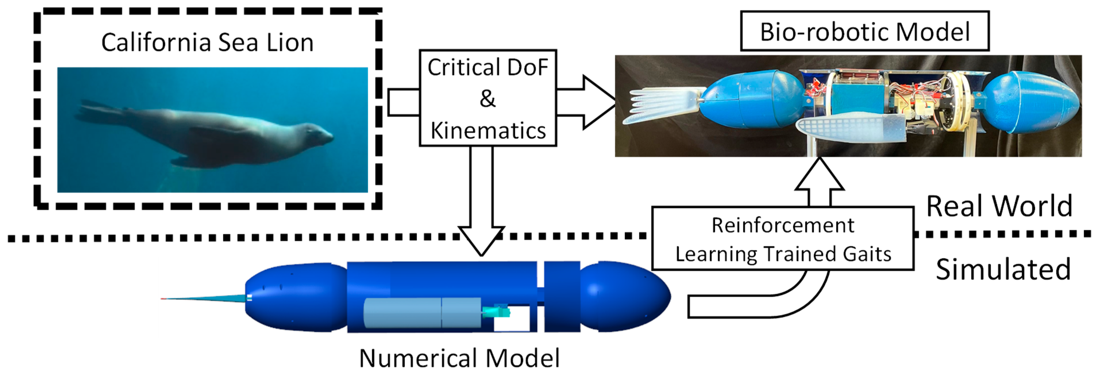
1. Introduction
2. Materials and Methods
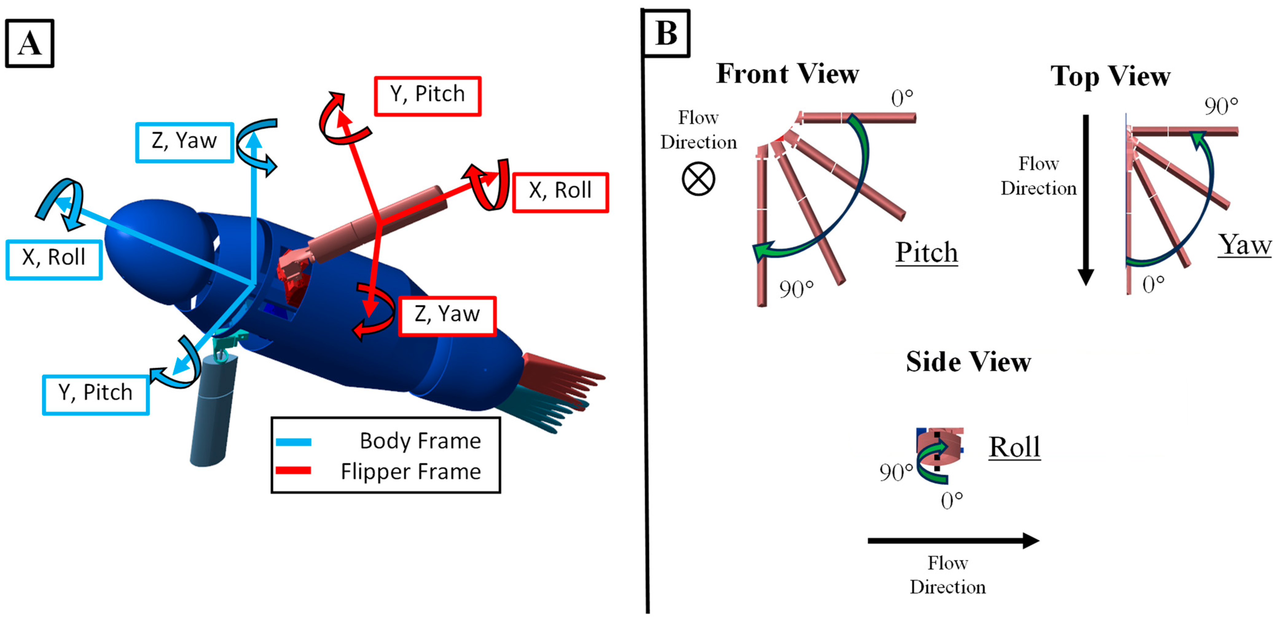
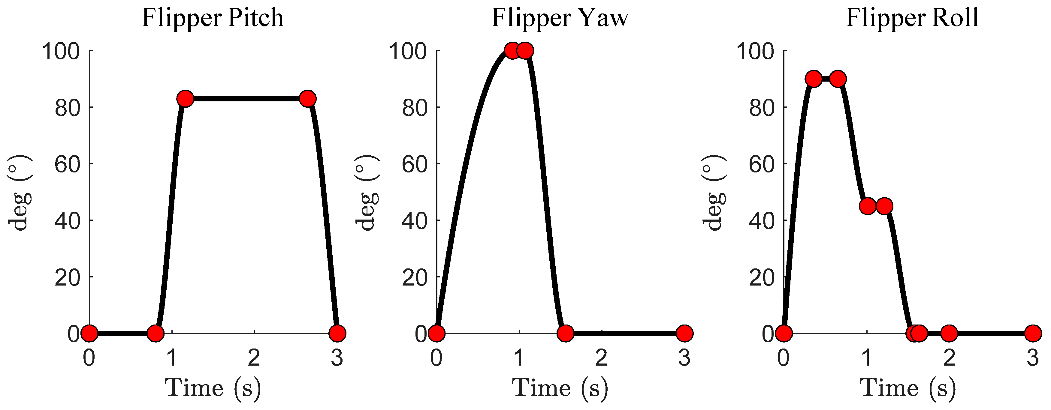
2.1. The Sea Lion Foreflipper Stroke Model
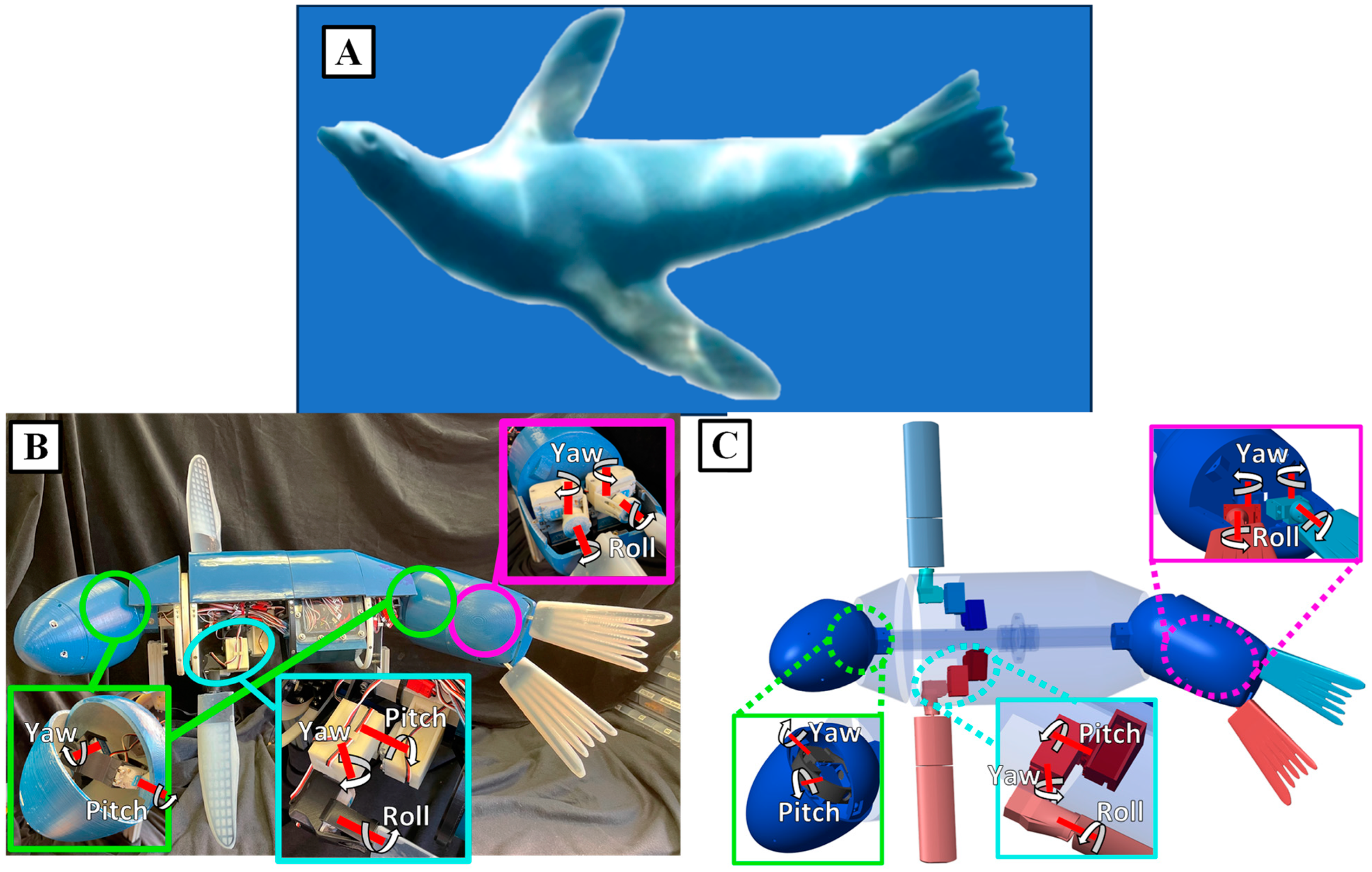
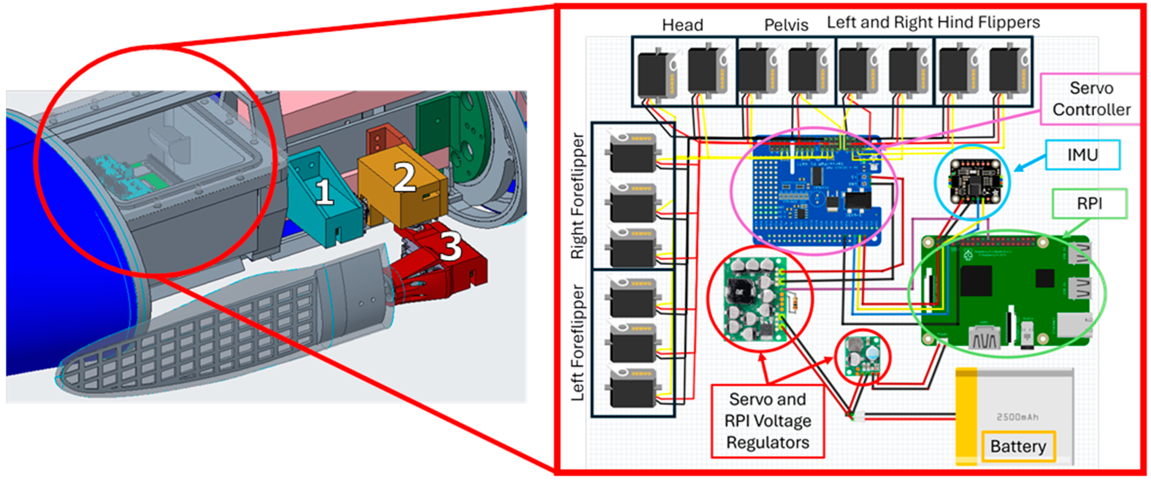
2.2. The Bio-Robotic Sealion
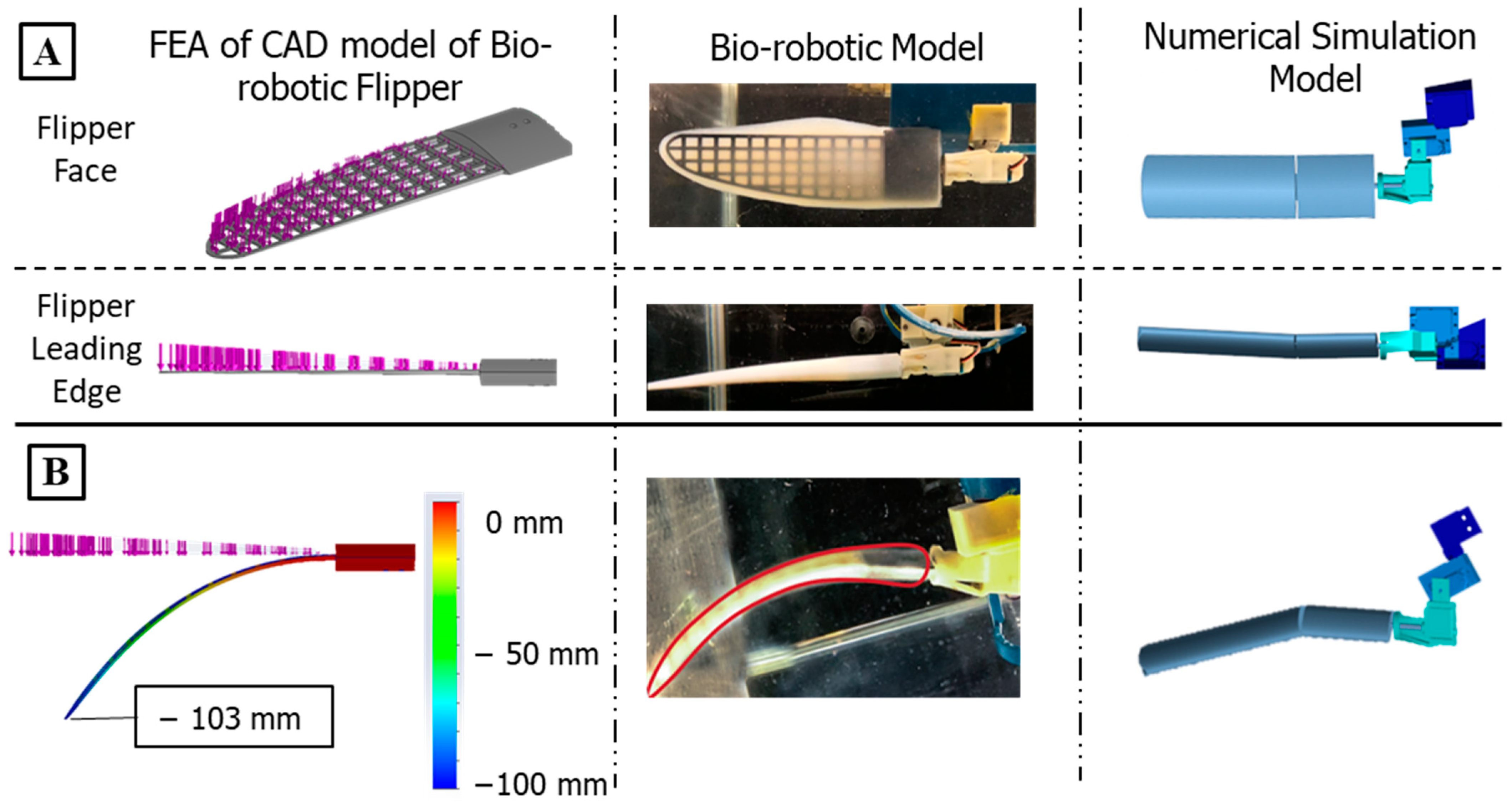
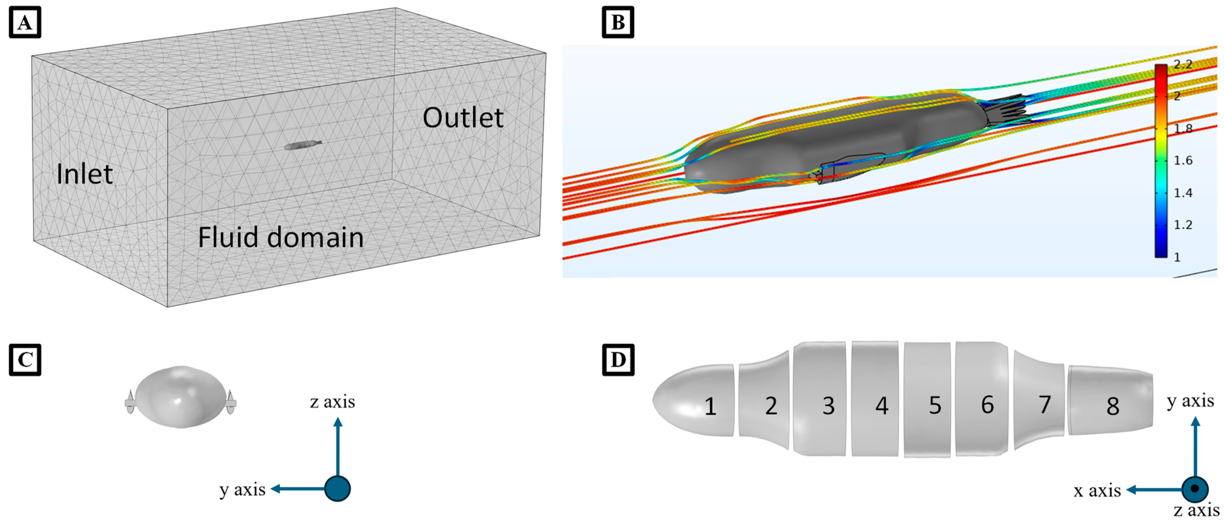
2.3. The Numerical Model of the Bio-Robotic Sea Lion
2.3.1. Hydrostatic Forces (Gravity and Buoyancy)
2.3.2. Hydrodynamic Forces (Drag and Added Mass)
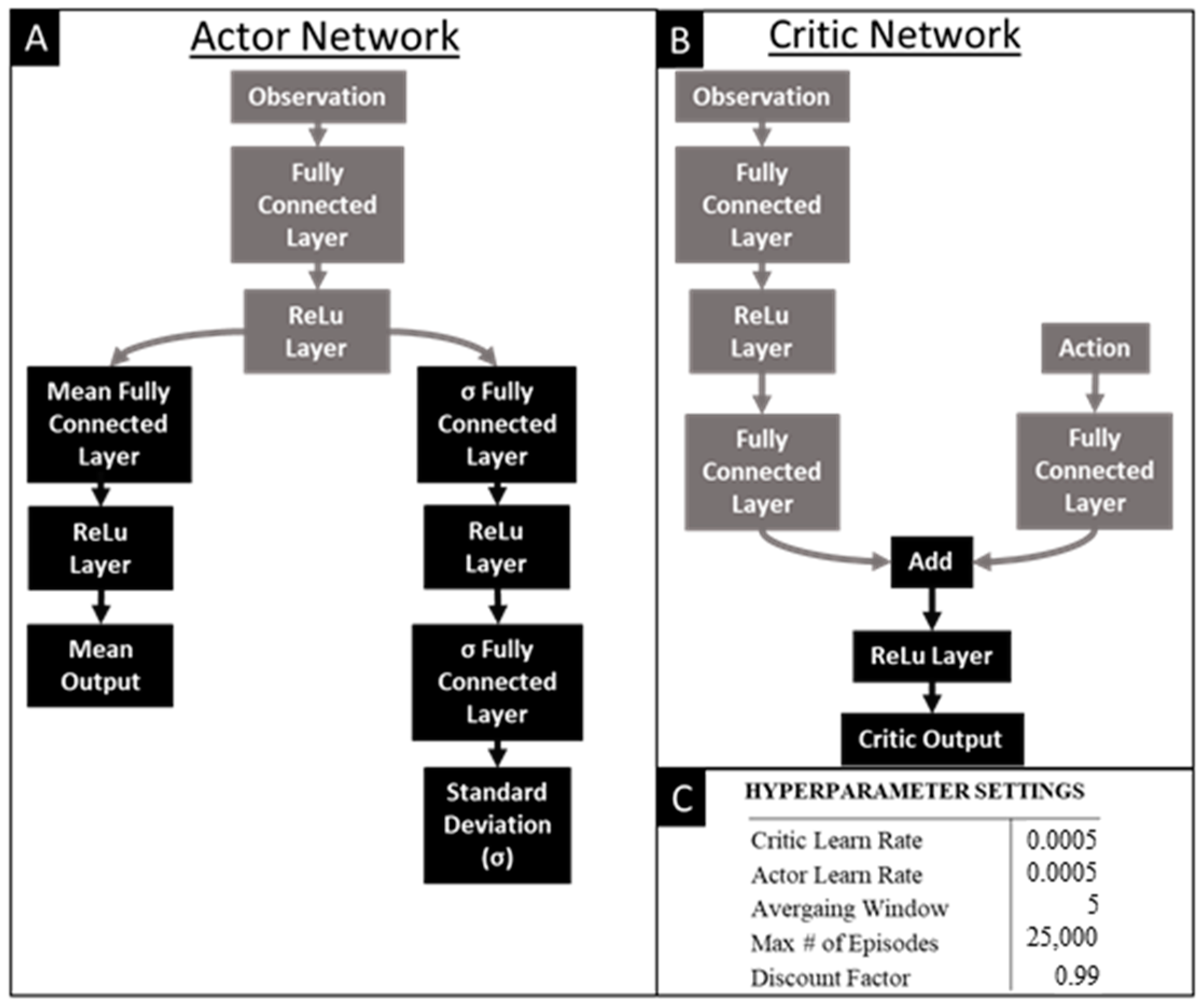
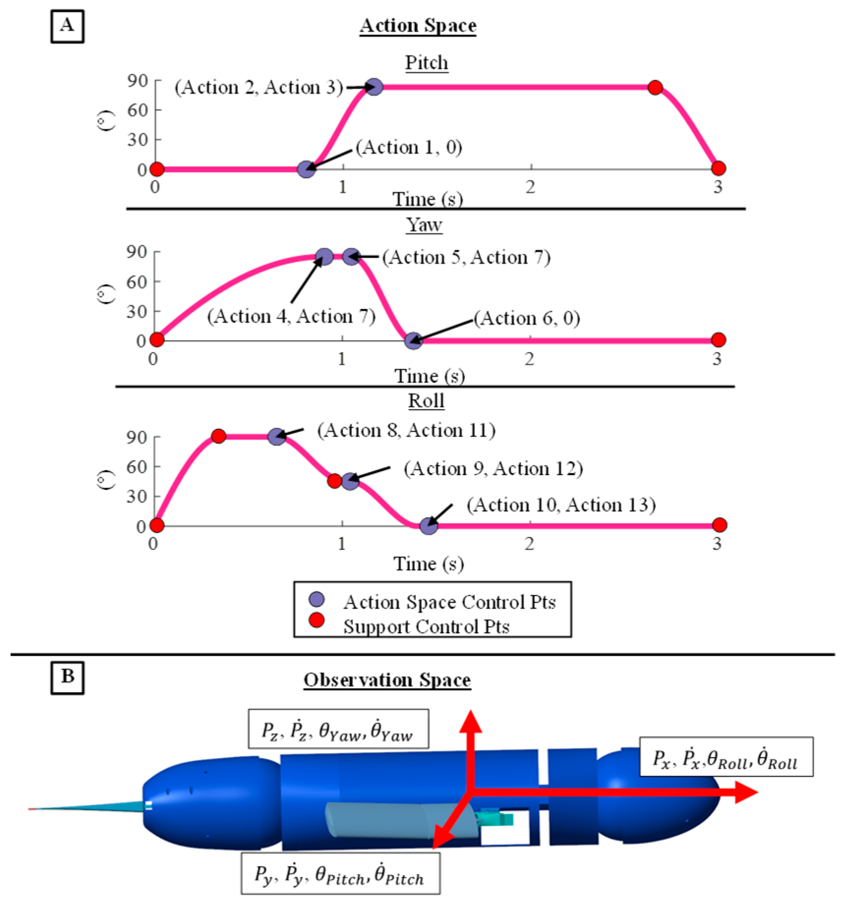
2.4. Reinforcement Learning
2.5. Experimental Setup and Data Collection
3. Results
3.1. Reinforcement Learning Convergence and Performance
3.2. Strokes Applied on Numerical Model
3.2.1. Translation in Simulation
3.2.2. Velocity in Simulation
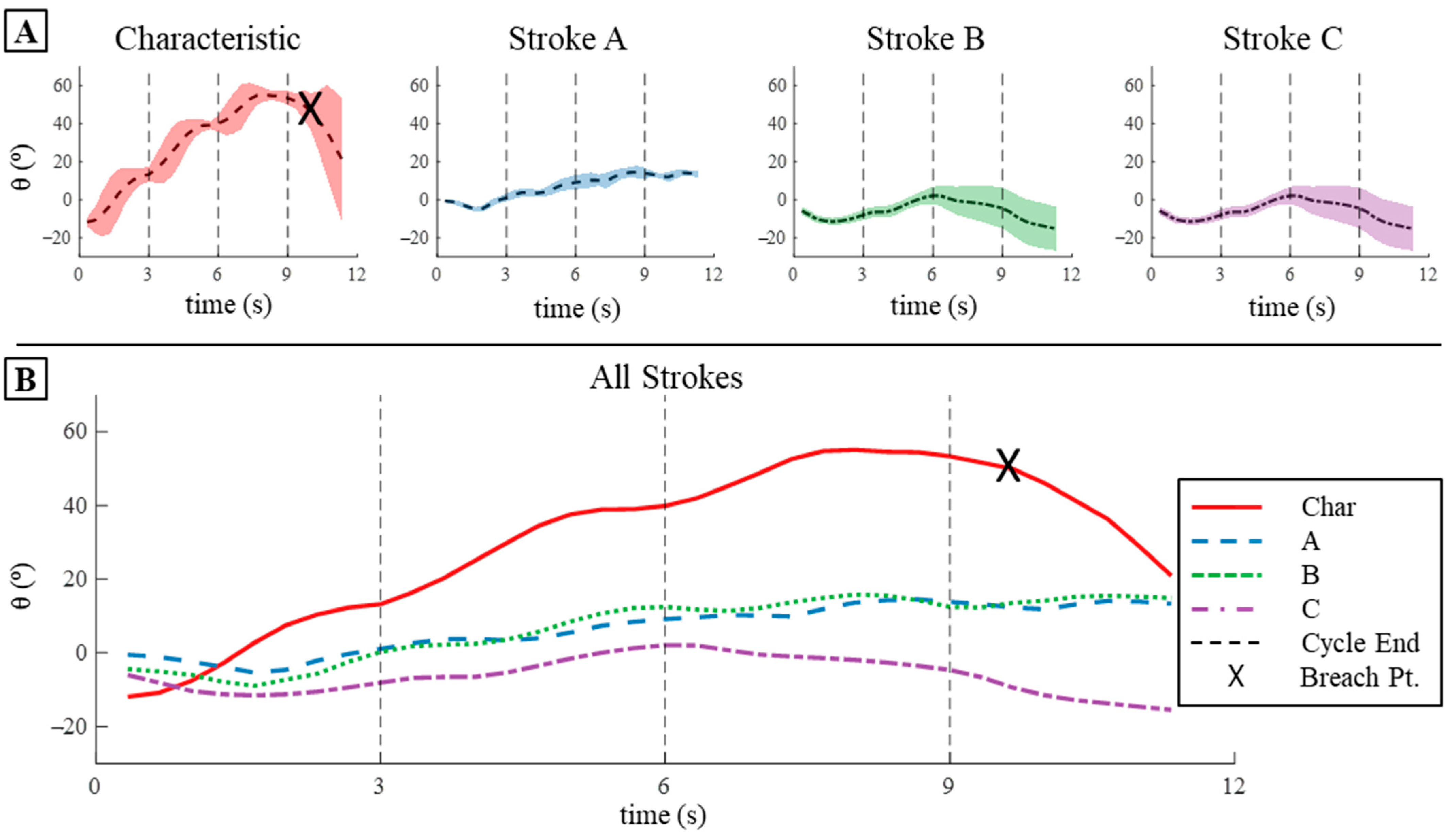
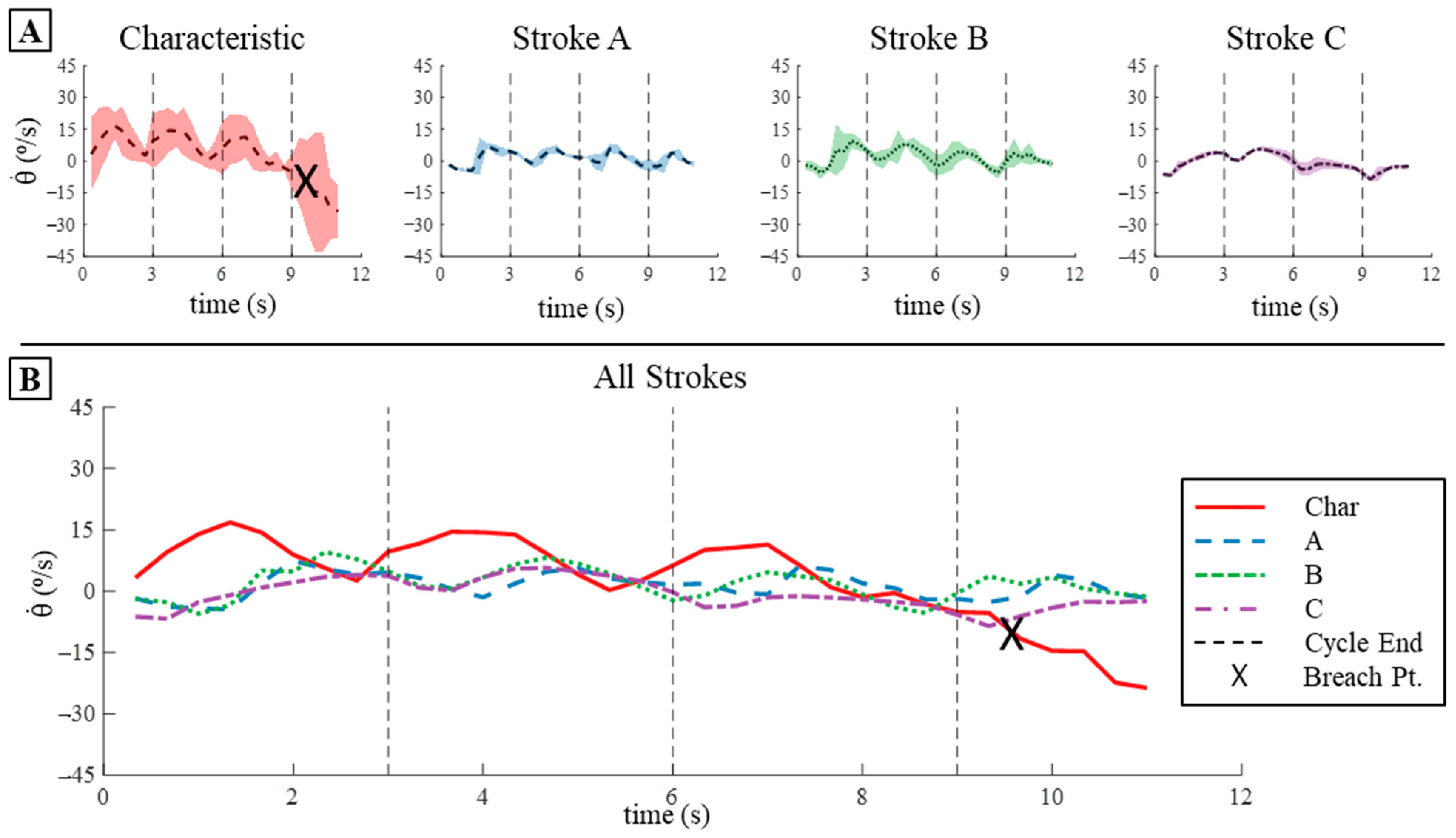
3.2.3. Pitch Displacement and Angular Velocity in Simulation
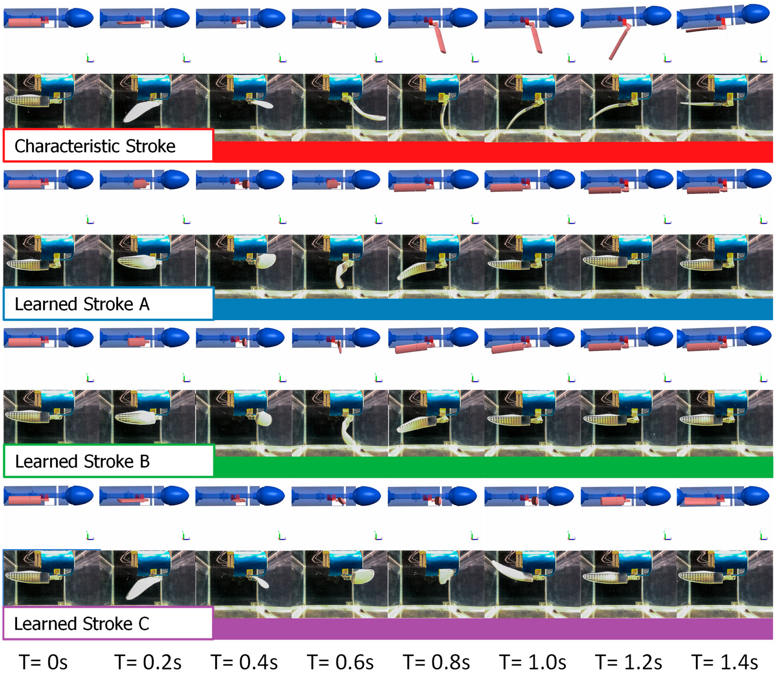
3.3. Strokes Applied on Bio-Robotic Platform
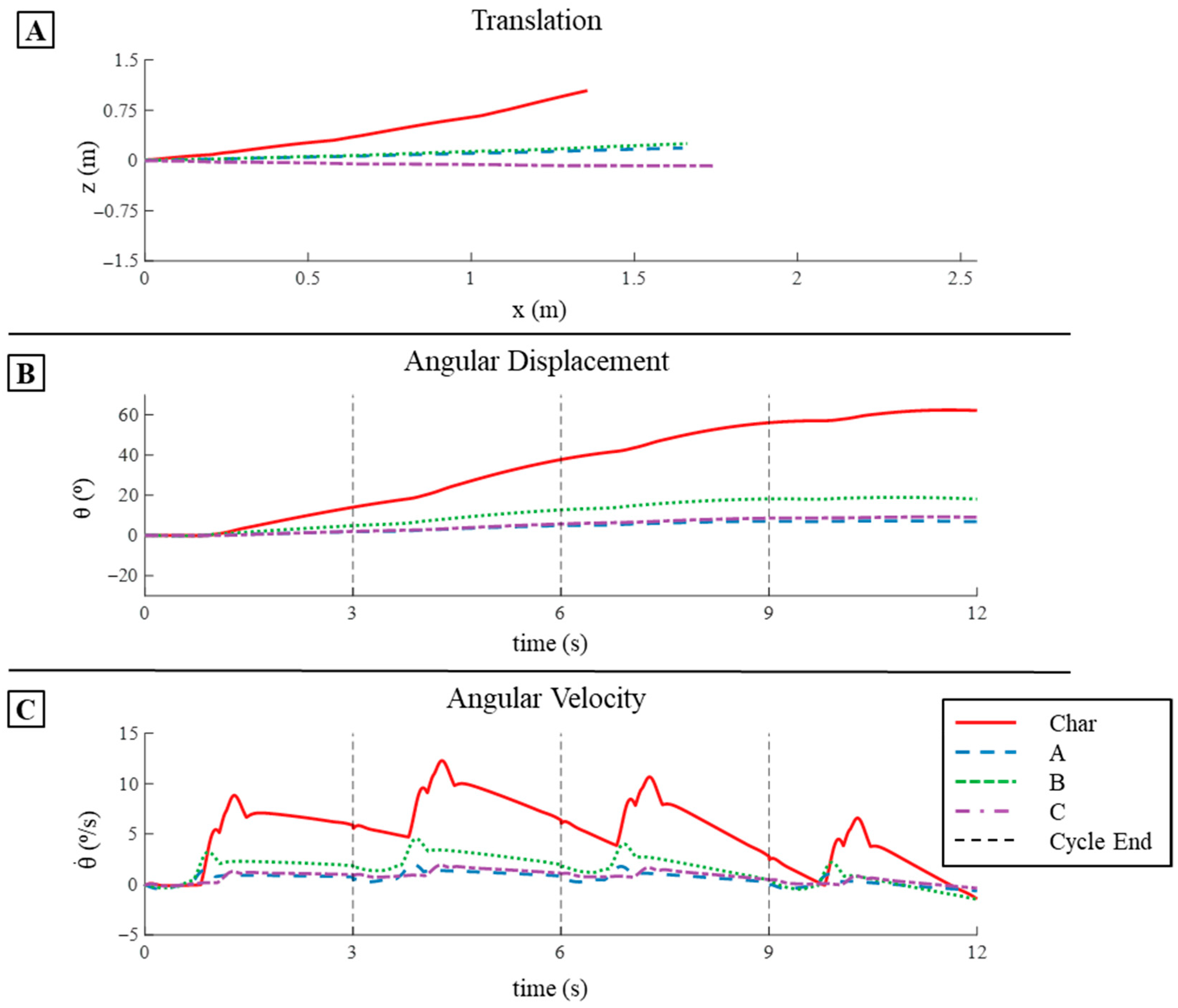
3.3.1. Translation on SEAMOUR
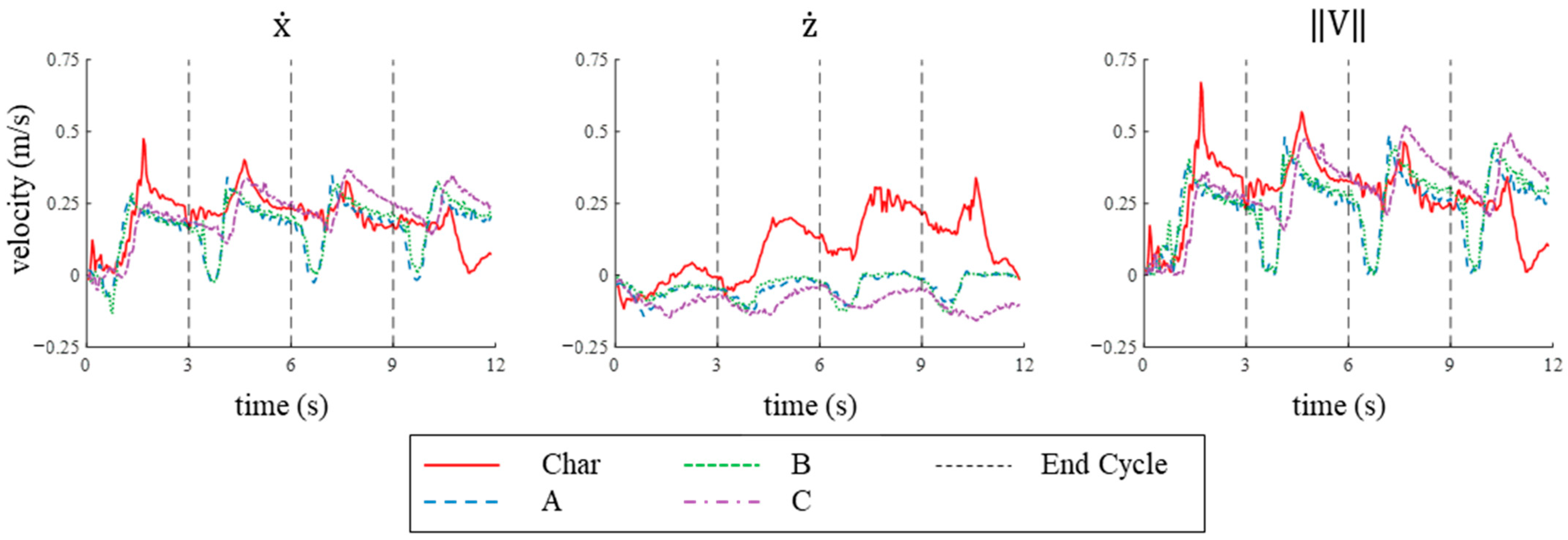
3.3.2. Velocity on SEAMOUR
3.3.3. Pitch Displacement and Angular Velocity on SEAMOUR
3.4. Comparative Analysis Numerical and Bio-Robotic Model
3.4.1. Displacement Comparison
3.4.2. Velocity Comparison
3.4.3. Pitch Displacement and Angular Velocity Comparison
4. Discussion and Conclusions
Supplementary Materials
Author Contributions
Funding
Institutional Review Board Statement
Data Availability Statement
Acknowledgments
Conflicts of Interest
References
- Wibisono, A.; Piran, M.J.; Song, H.K.; Lee, B.M. A Survey on Unmanned Underwater Vehicles: Challenges, Enabling Technologies, and Future Research Directions. Sensors 2023, 23, 7321. [Google Scholar] [CrossRef] [PubMed] [PubMed Central]
- Weihs, D. Stability Versus Maneuverability in Aquatic Locomotion. Integr. Comp. Biol. 2002, 42, 127–134. [Google Scholar] [CrossRef] [PubMed]
- Mignano, A.P.; Kadapa, S.; Tangorra, J.L.; Lauder, G.V. Passing the Wake: Using Multiple Fins to Shape Forces for Swimming. Biomimetics 2019, 4, 23. [Google Scholar] [CrossRef] [PubMed]
- Katzschmann, R.K.; Delpreto, J.; Maccurdy, R.; Rus, D. Exploration of Underwater Life with an Acoustically Controlled Soft Robotic Fish. 2018. Available online: http://robotics.sciencemag.org/ (accessed on 10 May 2024).
- Mignano, A.; Kadapa, S.; Drago, A.; Lauder, G.; Kwatny, H.; Tangorra, J. Fish robotics: Multi-fin propulsion and the coupling of fin phase, spacing, and compliance. Bioinspir. Biomim. 2024, 19, 026006. [Google Scholar] [CrossRef] [PubMed]
- Tangorra, J.; Phelan, C.; Esposito, C.; Lauder, G. Use of biorobotic models of highly deformable fins for studying the mechanics and control of fin forces in fishes. Integr. Comp. Biol. 2011, 51, 176–189. [Google Scholar] [CrossRef] [PubMed]
- Soliman, M.A.; Mousa, M.A.; Saleh, M.A.; Elsamanty, M.; Radwan, A.G. Modelling and implementation of soft bio-mimetic turtle using echo state network and soft pneumatic actuators. Sci. Rep. 2021, 11, 12076. [Google Scholar] [CrossRef] [PubMed]
- Zhang, J.; Chen, Y.; Liu, Y.; Gong, Y. Dynamic Modeling of Underwater Snake Robot by Hybrid Rigid-Soft Actuation. J. Mar. Sci. Eng. 2022, 10, 1914. [Google Scholar] [CrossRef]
- Fish, F.E.; Hurley, J.; Costa, D.P. Maneuverability by the sea lion Zalophus californianus: Turning performance of an unstable body design. J. Exp. Biol. 2003, 206, 667–674. [Google Scholar] [CrossRef] [PubMed]
- Feldkamp, S.D. Foreflipper propulsion in the California sea lion, Zalophus californianus. J. Zool. 1987, 212, 43–57. [Google Scholar] [CrossRef]
- Tan, J.; Zhang, T.; Coumans, E.; Iscen, A.; Bai, Y.; Hafner, D.; Bohez, S.; Vanhoucke, V. Sim-to-Real: Learning Agile Locomotion for Quadruped Robots. arXiv 2018, arXiv:1804.10332. [Google Scholar]
- Rodriguez, D.; Behnke, S. DeepWalk: Omnidirectional Bipedal Gait by Deep Reinforcement Learning. In Proceedings of the 2021 IEEE International Conference on Robotics and Automation (ICRA), Xi’an, China, 30 May–5 June 2021; IEEE: New York, NY, USA, 2021; pp. 3033–3039. [Google Scholar]
- Chen, G.; Lu, Y.; Yang, X.; Hu, H. Reinforcement learning control for the swimming motions of a beaver-like, single-legged robot based on biological inspiration. Robot. Auton. Syst. 2022, 154, 10411. [Google Scholar] [CrossRef]
- Carlucho, I.; De Paula, M.; Barbalata, C.; Acosta, G.G. A reinforcement learning control approach for underwater manipulation under position and torque constraints. In 2020 Global Oceans 2020; U.S. Gulf Coast, Institute of Electrical and Electronics Engineers Inc.: Singapore, 2020. [Google Scholar] [CrossRef]
- Drago, A.; Carryon, G.; Tangorra, J. Reinforcement Learning as a Method for Tuning CPG Controllers for Underwater Multi-Fin Propulsion. In Proceedings of the IEEE International Conference on Robotics and Automation, Philadelphia, PA, USA, 23–27 May 2022; Institute of Electrical and Electronics Engineers Inc.: New York, NY, USA, 2022; pp. 11533–11539. [Google Scholar] [CrossRef]
- Ju, H.; Juan, R.; Gomez, R.; Nakamura, K.; Li, G. Transferring policy of deep reinforcement learning from simulation to reality for robotics. Nat. Mach. Intell. 2022, 4, 1077–1087. [Google Scholar] [CrossRef]
- Körber, M.; Lange, J.; Rediske, S.; Steinmann, S.; Glück, R. Comparing Popular Simulation Environments in the Scope of Robotics and Reinforcement Learning. arXiv 2021, arXiv:2103.04616. [Google Scholar]
- van der Geest, N.; Garcia, L. Employing Robotics for the Biomechanical Validation of a Prosthetic Flipper for Sea Turtles as a Substitute for Animal Clinical Trials. Biomechanics 2023, 3, 401–414. [Google Scholar] [CrossRef]
- Fossen, T.I. Guidance and Control of Ocean Vehicles; John Wiley & Sons: Chichester, UK, 1995. [Google Scholar]
- Haarnoja, T.; Zhou, A.; Abbeel, P.; Levine, S. Soft Actor-Critic: Off-Policy Maximum Entropy Deep Reinforcement Learning with a Stochastic Actor. arXiv 2018, arXiv:1801.01290. [Google Scholar]


| Stroke Type | Cycle 1 | Cycle 2 | Cycle 3 | Cycle 4 | Mean | ||||||||||
|---|---|---|---|---|---|---|---|---|---|---|---|---|---|---|---|
| Char | 0.048 | 0.022 | 0.059 | 0.109 | 0.061 | 0.125 | 0.142 | 0.107 | 0.179 | 0.153 | 0.157 | 0.221 | 0.113 | 0.087 | 0.146 |
| A | 0.052 | 0.005 | 0.063 | 0.118 | 0.012 | 0.119 | 0.170 | 0.019 | 0.172 | 0.209 | 0.025 | 0.210 | 0.137 | 0.015 | 0.141 |
| B | 0.052 | 0.005 | 0.062 | 0.119 | 0.015 | 0.120 | 0.172 | 0.026 | 0.174 | 0.211 | 0.037 | 0.214 | 0.139 | 0.021 | 0.143 |
| C | 0.047 | −0.004 | 0.165 | 0.121 | −0.008 | 0.121 | 0.183 | −0.009 | 0.183 | 0.232 | −0.006 | 0.232 | 0.146 | −0.007 | 0.147 |
| Stroke Type | Cycle 1 | Cycle 2 | Cycle 3 | Cycle 4 | Mean | |||||
|---|---|---|---|---|---|---|---|---|---|---|
| || | ||||||||||
| Characteristic | 14.03 | 4.68 | 23.71 | 7.91 | 18.3 | 6.1 | 6.04 | 2.02 | 15.52 | 5.18 |
| A | 1.86 | 0.62 | 3.08 | 1.03 | 2.15 | 0.72 | −0.25 | −0.09 | 1.83 | 0.61 |
| B | 4.86 | 1.62 | 7.87 | 2.62 | 5.45 | 1.82 | −0.1 | −0.03 | 4.57 | 1.52 |
| C | 2.02 | 0.68 | 3.72 | 1.24 | 2.87 | 0.96 | 0.48 | 0.16 | 2.27 | 0.76 |
| Stroke Type | Cycle 1 | Cycle 2 | Cycle 3 | Cycle 4 | Mean | ||||||||||
|---|---|---|---|---|---|---|---|---|---|---|---|---|---|---|---|
| Char | 0.179 | −0.027 | 0.199 | 0.256 | 0.087 | 0.284 | 0.215 | 0.189 | 0.295 | 0.137 | 0.144 | 0.202 | 0.198 | 0.098 | 0.245 |
| A | 0.135 | −0.064 | 0.171 | 0.178 | −0.051 | 0.199 | 0.178 | −0.027 | 0.193 | 0.175 | −0.022 | 0.19 | 0.166 | −0.041 | 0.188 |
| B | 0.125 | −0.047 | 0.161 | 0.184 | −0.043 | 0.204 | 0.194 | −0.031 | 0.212 | 0.202 | −0.03 | 0.217 | 0.176 | −0.037 | 0.199 |
| C | 0.118 | −0.09 | 0.165 | 0.228 | −0.091 | 0.251 | 0.259 | −0.076 | 0.272 | 0.246 | −0.115 | 0.274 | 0.213 | −0.093 | 0.241 |
| Stroke Type | Cycle 1 | Cycle 2 | Cycle 3 | Cycle 4 | Mean | |||||
|---|---|---|---|---|---|---|---|---|---|---|
| || | | | | |||||||||
| Characteristic | −1.48 | 1.38 | 27.22 | 10.61 | 18.17 | 6.77 | −33.8 | −9.24 | 20.17 | 7.00 |
| A | −0.16 | 0.40 | 7.33 | 2.68 | 5.41 | 1.57 | −0.5 | −0.22 | 3.35 | 1.22 |
| B | 1.55 | 2.06 | 22.95 | 3.30 | 12.45 | 0.20 | 2.53 | 1.27 | 9.87 | 1.71 |
| C | −9.84 | −3.04 | 8.9 | 3.50 | −1.96 | −0.88 | −12.75 | −4.25 | 8.36 | 2.92 |
Disclaimer/Publisher’s Note: The statements, opinions and data contained in all publications are solely those of the individual author(s) and contributor(s) and not of MDPI and/or the editor(s). MDPI and/or the editor(s) disclaim responsibility for any injury to people or property resulting from any ideas, methods, instructions or products referred to in the content. |
© 2024 by the authors. Licensee MDPI, Basel, Switzerland. This article is an open access article distributed under the terms and conditions of the Creative Commons Attribution (CC BY) license (https://creativecommons.org/licenses/by/4.0/).
Share and Cite
Drago, A.; Kadapa, S.; Marcouiller, N.; Kwatny, H.G.; Tangorra, J.L. Using Reinforcement Learning to Develop a Novel Gait for a Bio-Robotic California Sea Lion. Biomimetics 2024, 9, 522. https://doi.org/10.3390/biomimetics9090522
Drago A, Kadapa S, Marcouiller N, Kwatny HG, Tangorra JL. Using Reinforcement Learning to Develop a Novel Gait for a Bio-Robotic California Sea Lion. Biomimetics. 2024; 9(9):522. https://doi.org/10.3390/biomimetics9090522
Chicago/Turabian StyleDrago, Anthony, Shraman Kadapa, Nicholas Marcouiller, Harry G. Kwatny, and James L. Tangorra. 2024. "Using Reinforcement Learning to Develop a Novel Gait for a Bio-Robotic California Sea Lion" Biomimetics 9, no. 9: 522. https://doi.org/10.3390/biomimetics9090522
APA StyleDrago, A., Kadapa, S., Marcouiller, N., Kwatny, H. G., & Tangorra, J. L. (2024). Using Reinforcement Learning to Develop a Novel Gait for a Bio-Robotic California Sea Lion. Biomimetics, 9(9), 522. https://doi.org/10.3390/biomimetics9090522