Abstract
Based on a meta-heuristic secretary bird optimization algorithm (SBOA), this paper develops a multi-strategy improvement secretary bird optimization algorithm (MISBOA) to further enhance the solving accuracy and convergence speed for engineering optimization problems. Firstly, a feedback regulation mechanism based on incremental PID control is used to update the whole population according to the output value. Then, in the hunting stage, a golden sinusoidal guidance strategy is employed to enhance the success rate of capture. Meanwhile, to keep the population diverse, a cooperative camouflage strategy and an update strategy based on cosine similarity are introduced into the escaping stage. Analyzing the results in solving the CEC2022 test suite, the MISBOA both get the best comprehensive performance when the dimensions are set as 10 and 20. Especially when the dimension is increased, the advantage of MISBOA is further expanded, which ranks first on 10 test functions, accounting for 83.33% of the total. It illustrates the introduction of improvement strategies that effectively enhance the searching accuracy and stability of MISBOA for various problems. For five real-world optimization problems, the MISBOA also has the best performance on the fitness values, indicating a stronger searching ability with higher accuracy and stability. Finally, when it is used to solve the shape optimization problem of the combined quartic generalized Ball interpolation (CQGBI) curve, the shape can be designed to be smoother according to the obtained parameters based on MISBOA to improve power generation efficiency.
1. Introduction
Optimization problems in engineering design are to select a set of parameters (variables) to achieve the optimal value of the design index (goal) under a series of relevant constraints [1]. Those confusions widely exist in various fields, such as production cost optimization [2], public transportation optimization [3], production decision optimization [4], structural design optimization [5], feature selection [6], path planning [7], and so on.
To solve those complex optimization problems effectively, meta-heuristic algorithms (MHAs) are studied and proposed, the core idea of which is to gradually approach the optimal solution of the problem by searching in the problem space [8]. Different from optimization algorithms based on precise gradient information or Hesse matrix, the main advantage of MHAs is that they can handle complex, non-linear problems and do not require assumptions about the specific model of the problem [9]. Furthermore, with the continuous development and improvement of computer hardware and software, MHAs have shown strong ability to solve practical problems, and the future development prospects will be broader [10].
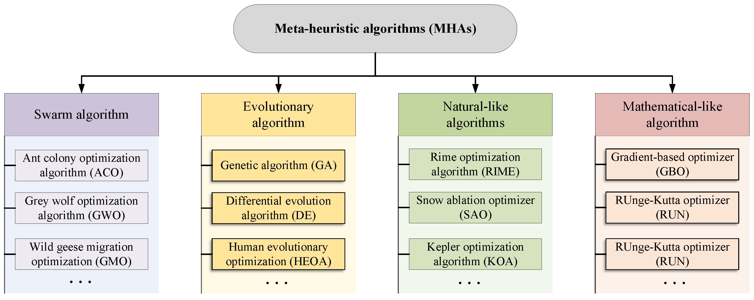
As shown in Figure 1, according to different search mechanisms, MHAs are usually classified into four types, which are swarm algorithms, evolutionary algorithms, natural-like algorithms, and mathematical-like algorithms [11]. For swarm algorithms, they currently are the most popular MHAs, inspired by the adaptive, self-organizing group behaviors exhibited by social species in nature, such as foraging, hunting, working, or migrating [12]. For example, in the classical ant colony optimization algorithm (ACO), the foraging behavior based on pheromone concentration in the ant group is modeled mathematically to form a basic search framework [13]. Grey wolf optimization algorithm (GWO) was constructed by simulating the hunting behavior of grey wolves, belonging to swarm algorithms. Based on the hierarchical mechanism and hunting behavior, the special mechanism has achieved good results in balanced exploration and development of GWO, leading to good performance in convergence speed and solution accuracy [14]. Inspired by the migratory behavior of wild geese, a wild geese migration optimization (GMO) algorithm was developed. During the long-distance migration, they usually keep a special formation consisting of several small groups [15]. Evolutionary algorithms are constructed by the natural law of survival of the fittest [16]. For genetic algorithm (GA), it simulated theory of Darwinian biological evolution, mainly including natural selection and genetic mechanisms [17]. Differential evolution algorithm (DE) was also a representative of this type. It is inspired by the mutation strategy, hybridization strategy, and selection operations [18]. Different from GA, each individual in the DE corresponds to a solution vector, and the complex encoding and decoding process is abandoned. Human evolutionary optimization algorithm (HEOA) was inspired by the human evolution process, mainly consisting of two distinct phases: human exploration and human development [19]. Natural-like algorithms are developed by modeling common natural phenomena, such as rain, snow, wind, and so on [20]. For example, inspired by the mechanism of frost and ice growth in nature, a novel rime optimization algorithm (RIME) was proposed in 2023. By studying the various growth processes of rime-ice, this algorithm develops a novel searching frame, including soft-rime search and hard-rime puncture strategies [21]. A snow ablation optimizer (SAO) was constructed in 2022, which mainly emulates the sublimation and melting behavior of snow to realize a balance between exploitation and exploration in the solution space and discourage premature convergence [22]. The Kepler optimization algorithm (KOA) was also a well-known approach of natural-like algorithms based on the celestial motion principle, which simulates the motion law of planets around the sun to solve the optimization problem [23]. The last category is mathematical-like algorithms, mainly including the sine cosine algorithm (SCA) [24], gradient-based optimizer (GBO) [25], and Runge Kutta optimizer (RUN) [26]. The SCA only uses the volatility and periodicity of sine and cosine functions as the design goal of the operator to search and iterate the optimal solution. Compared with the GA, SCA has the advantages of fewer parameters, a simple structure, and easy implementation. For the GBO, it adopts a gradient-based approach to improve exploration trends and accelerate convergence to obtain better bits in the search space.

Figure 1.
The classification of MHAs.
Though optimization algorithms can be solved by various MHAs, the accuracy and efficiency are different due to diverse algorithm structures. Thus, to enhance the performance of original algorithms, different improved versions of the basic MHAs are introduced [27]. Here, two common types of improvement methods are discussed. In the first class, hybrid algorithms are constructed by mixing different basic algorithms with various characters [28]. For example, Nenavath and Jatoth proposed a new hybrid SCA-DE by mixing the SCA and differential DE [29]. Compared with the basic SCA and DE, the proposed hybrid algorithm has better capability to escape from local optima with faster convergence. Garg also presented a hybrid algorithm named PSO-GA for solving constrained optimization problems. It adopted the direction of particle swarm optimization (PSO) and the decision operators of GA, leading to better balance between the exploration and exploitation abilities [30]. However, this kind of method may inherit their own absence when combining the advantages of different algorithms, which means certain limitations on the improvement effect. Thus, another kind of method is studied, that is, several improvement strategies are incorporated into the original algorithms. For example, aiming to overcome the shortcomings of low accuracy, slow convergence speed, and easily falling into local optimums, Hu et al. proposed an improved BWO algorithm by introducing novel selecting strategies, mutation methods, and adaptive parameters [31]. The proposed algorithm achieved higher classification accuracy while using fewer information from the original datasets. Liu et al. proposed an enhanced grey wolf optimization algorithm (NAS-GWO) for the agricultural UAV trajectory planning problem [32]. The improved algorithm mainly includes three key strategies. A boundary constraint mechanism is adopted to enhance the ability of achieving better solutions. The typical Gaussian mutation model and spiral function are used to reduce the possibility of being troubled with local optimums. Meanwhile, to keep the balance of exploitation and exploration abilities, the NAS-GWO hires a nonlinear factor based on the Sigmoid function.
In this paper, a novel secretary bird optimization algorithm (SBOA) proposed in 2024, is analyzed and studied. By being tested on CEC2017 and CEC2022 benchmark test suites, the searching accuracy, convergence rate, and stability of SBOA have been verified [33]. However, limited by the single structure of the original algorithm, there is still room to develop an enhanced version to get better solutions. Thus, by introducing targeted improvement strategies, we propose a multi-strategy secretary bird optimization algorithm (MISBOA). The main contributions can be summarized as follows:
- (1)
- An enhanced algorithm MISBOA is proposed by integrating four specific improvement strategies.A feedback regulation mechanism is introduced to fully make use of the global information, leading to faster global convergence.To improve the development ability of SBOA, a golden sinusoidal guidance strategy is adopted in the hunting stage.In the escape stage, a cooperative camouflage strategy is employed to enhance the global exploration ability.An update strategy based on cosine similarity is used to keep the population diverse, which influences the ability to escape local optimums.
- (2)
- The ability of MISBOA is verified by solving basic test functions and well-known engineering optimization problems.The MISBOA and other eight typical algorithms are tested on functions with 10 and 20 dimensions of CEC2022. Accuracy, convergence speed, stability, and extensibility of various algorithms are analyzed.The engineering application capability of the MISBOA is verified on five complex engineering optimization problems.
- (3)
- The MISBOA is applied for a shape optimization problem of combined curves.With the aim of minimizing the total energy, a shape optimization model of combined quartic generalized Ball interpolation (CQGBI) curve is established.The shape of wind-driven generator blades is optimized by MISBOA and other algorithms to increase the efficiency of power generation.
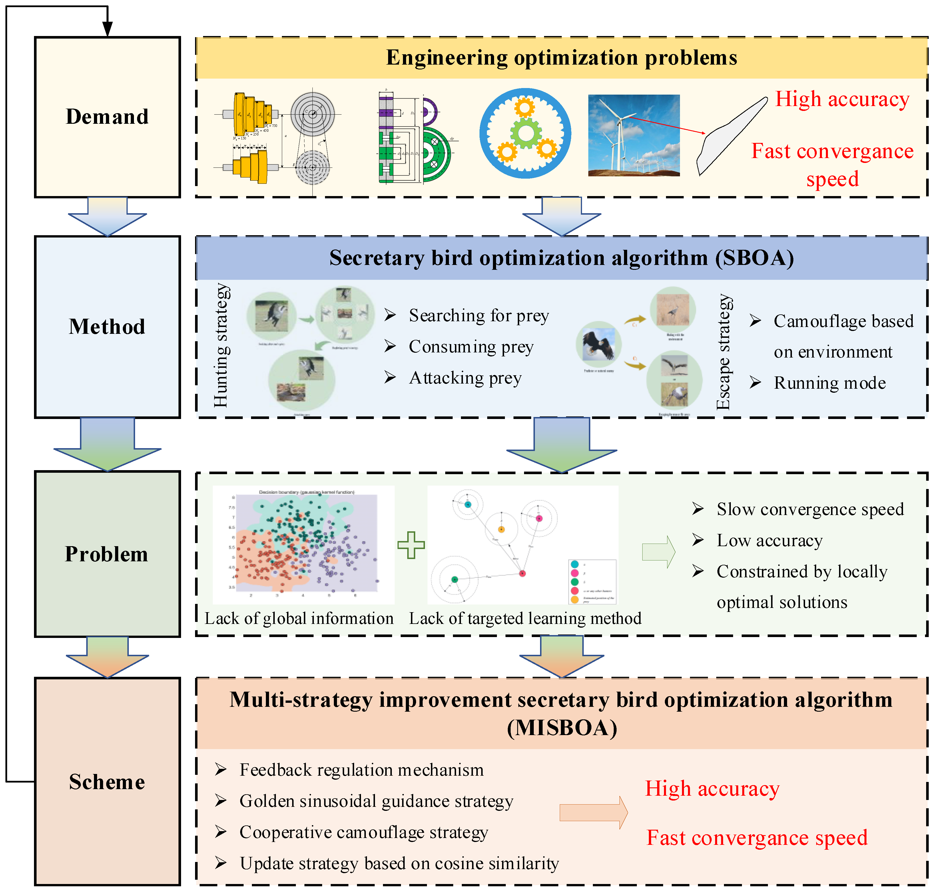
Figure 2 shows the motivation of this paper to illustrate the idea and value of the research more intuitively. The organization of our work can be summarized as follows: Section 2 introduces the original SBOA algorithm and the detailed steps for constructing the MISBOA. Section 3 analyzes the performance of MISBOA according to the results of the CEC2022 test suit. Section 4 tests the ability of MISBOA in solving engineering optimization problems and the established shape optimization model of combined quartic generalized Ball interpolation. In Section 5, the main conclusions of this paper and future work are given.
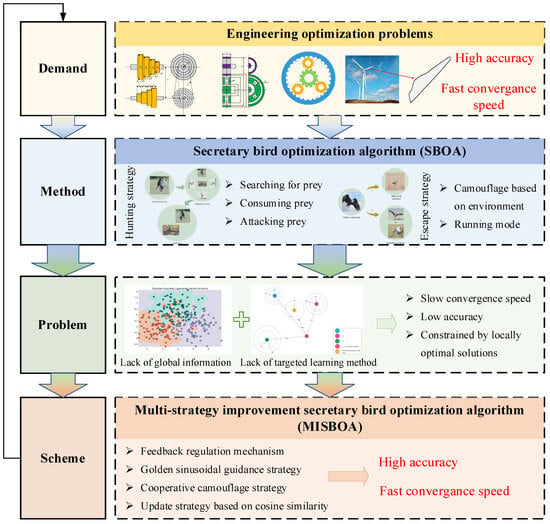
Figure 2.
The motivation of this paper.
2. The Multi-Strategy Improvement Secretary Bird Optimization Algorithm
2.1. The Basic Secretary Bird Optimization Algorithm
Secretary birds are large terrestrial raptors, usually inhabit tropical savannas or semi-desert areas. They are natural enemies of snakes on the African continent, such as the black mamba, cobra, and others. Inspired by their survival strategy of searching for prey and evading pursuit from predators in harsh environments, a secretary bird optimization algorithm is constructed to deal with complex optimization problems. The SBOA consists of the following parts:
2.1.1. Initial Preparation Phase
Firstly, for a typical minimization optimization problem , the initial solutions used to start the search needs to be determined. Here, N initial solutions form the initial population of secretary birds. Each individual Xi in the population corresponds to a solution to the optimization problem, which is initialized by Equation (1).
where lb and ub are the lower and upper bounds of the decision variables. rand represents a random number in [0, 1]. M is the dimension of the problem. In addition, the fitness value of the solution Xi is noted as to measure its quality.
2.1.2. Hunting Strategy of Secretary Birds
Unlike other fierce predators, secretary birds adopt a more intelligent approach to hunting snakes. After spotting the target, they do not dive down and fight straightaway, but wander, jump, and pick quarrels near the snake patiently to observe and confuse opponents. Until a suitable time, they will strike quickly and kill the prey. Thus, the whole hunting process can be divided into three steps, which are searching for prey, consuming prey, and attacking prey. Then, mathematical models are used to characterize these stages.
- (1)
- Searching for prey
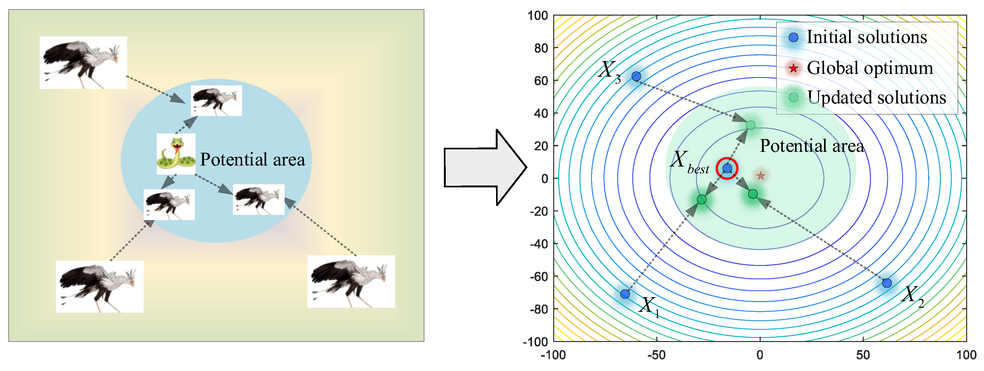
In this stage, the secretary birds need to search for prey at a safe distance. For optimization algorithms, this initial stage asks for stronger exploration ability to acquire enough information for the whole search area. As shown in Figure 3, the secretary bird can explore new potential areas by referring to the positions of the other two secretary birds. Therefore, differential mutation operations are introduced to keep enhancing algorithm diversity. For each individual Xi, it will use Equations (2) and (3) to update position when the current iteration time t is smaller than one-third of the maximum iterations T.
where , are two individuals randomly selected from the current population. R1 is a random vector, including 1 × M elements randomly selected in [0, 1].
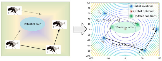
Figure 3.
The modeling process of searching for prey.
- (2)
- Consuming prey
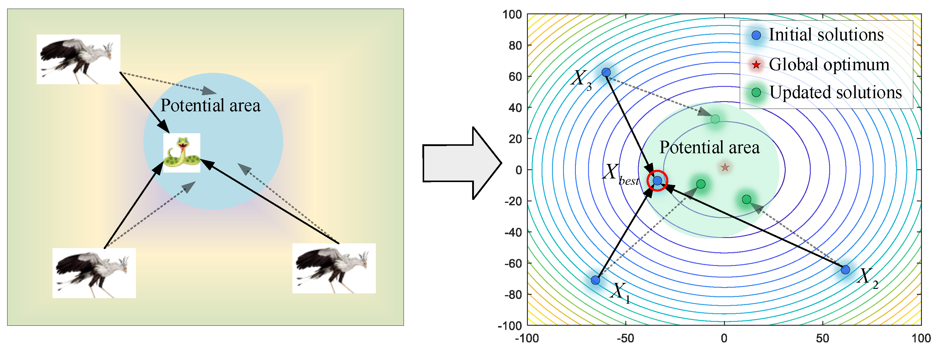
Once secretary birds find potential prey, they first hover around the snake with agile footwork and maneuvers. By watching and luring opponents in the process of circling, the patience of the prey will be consumed to let down its guard. As shown in Figure 4, by regarding the current best individual as the prey, other secretary birds update their position to close the prey. In this way, the success of hunting will be greatly improved. When , the Brownian motion (RB) is applied to model the random movement of the secretary birds, as shown in Equation (4),
where randn(1,M) is a randomly generated vector satisfying the standard normal distribution, whose mean value is 0 and standard deviation is 1.
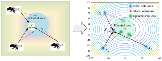
Figure 4.
The modeling process of consuming prey.
Then, secretary birds update their positions by Equations (5) and (6).
where Xbest is the best solution for the current population.
- (3)
- Attacking prey
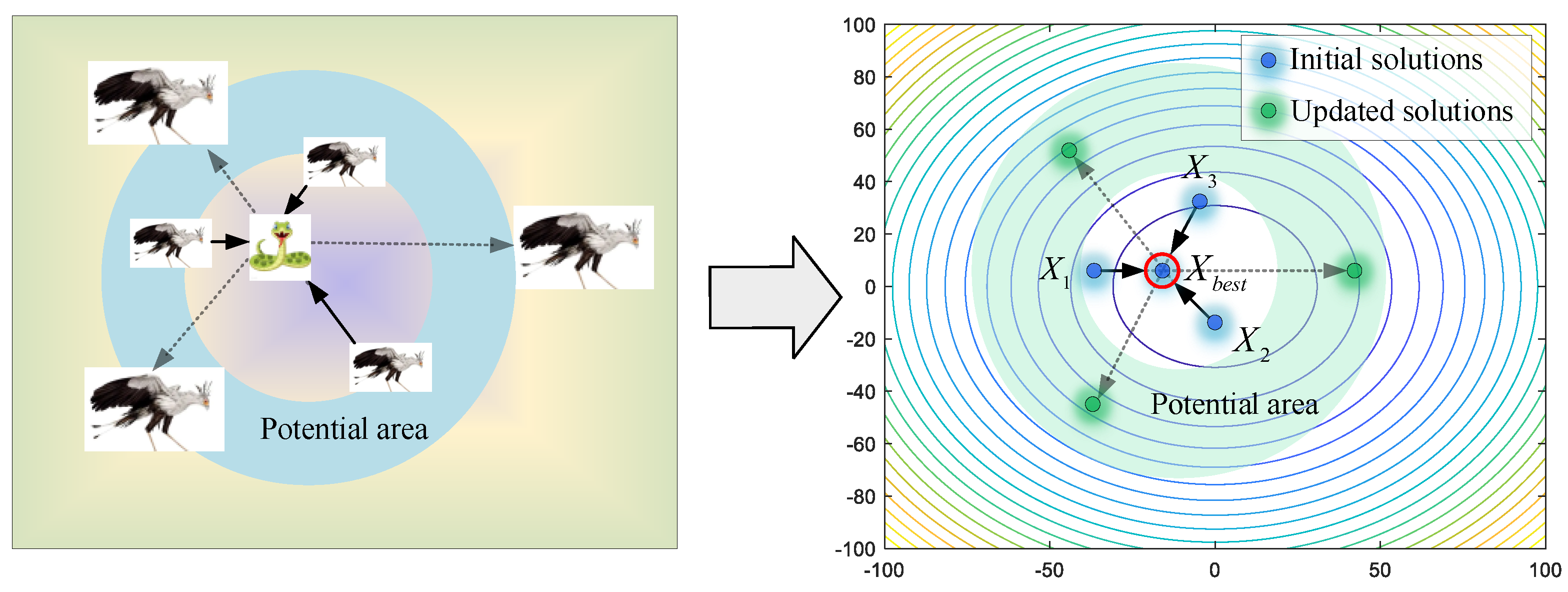
After constant consumption, the prey will be exhausted. It is time for secretary birds to start the attack. Here, the levy flight strategy is used to simulate various attack ways, such as continuous steps and occasional long jumps in a short time. Equations (7) and (8) are used to describe the characters of this stage. As shown in Figure 5, secretary birds quickly approach the prey, meaning candidate solutions are close to the current best solution. When , this strategy will be executed.
where RL represents the levy flight strategy, which is
where , in which s and φ are fixed numbers of 0.01 and 1.5, respectively. u and υ are random numbers in [0, 1]. σ is set as follows.
where is the gamma function and η is set as 0.5.
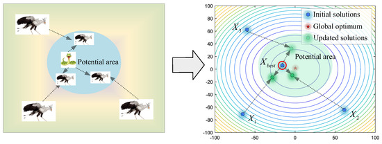
Figure 5.
The modeling process of attacking prey.
2.1.3. Escape Strategy for Secretary Birds
In nature, secretary birds also face the risk of being hunted when hunting other prey. The main enemies they need to face are eagles, hawks, foxes, and jackals. When they sense danger, various evasion strategies are necessary to protect themselves or their food. In this algorithm, camouflage and running modes are modeled to simulate the escape strategies.
- (1)
- Camouflage based on environment
Facing enemies, the secretary birds first choose to camouflage themselves to avoid danger. As shown in Figure 6, secretary birds update their positions around the prey (best individual), reflecting the behavior of trying to escape local optimums in the algorithms. The mathematical model of this strategy is shown in Equations (11) and (12).
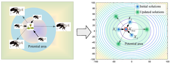
Figure 6.
The modeling process of camouflage based on environment.
- (2)
- Running mode
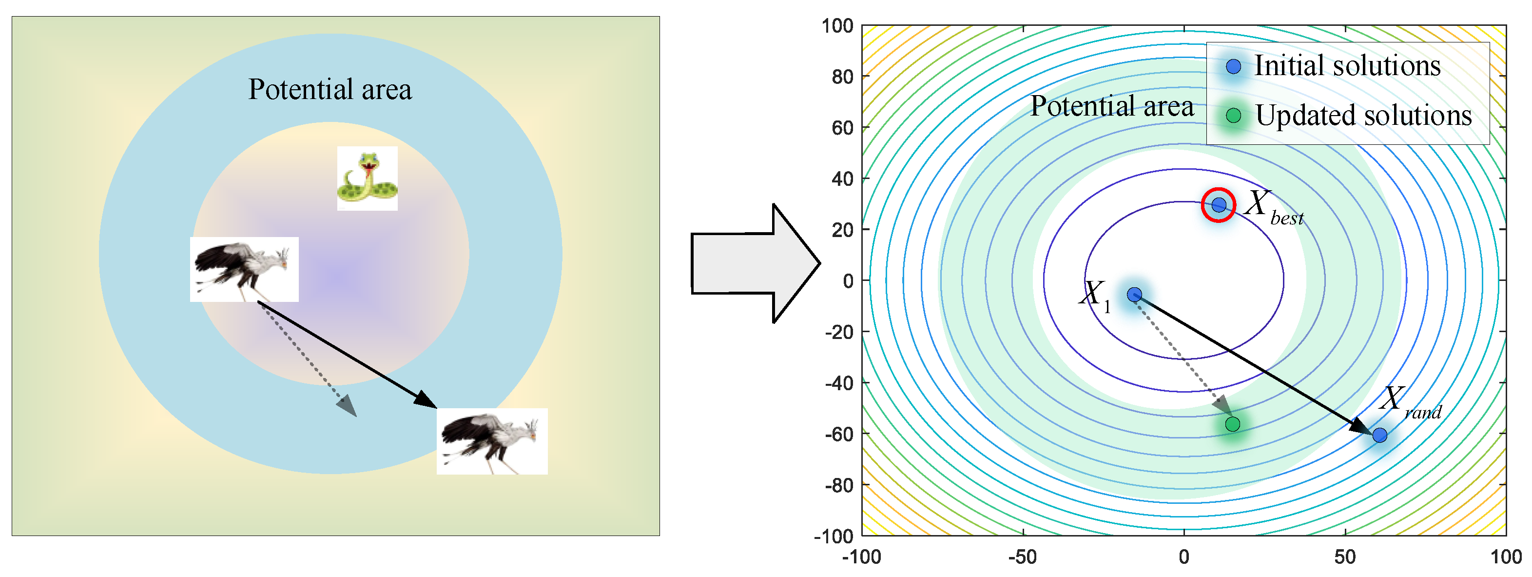
If they cannot avoid the enemy, flight or rapid-running strategies will be employed to keep them safe. As shown in Figure 7, a random individual Xrand is selected as the leader for reference, avoiding being limited to local optimums. Secretary birds update their positions by Equations (13) and (14).
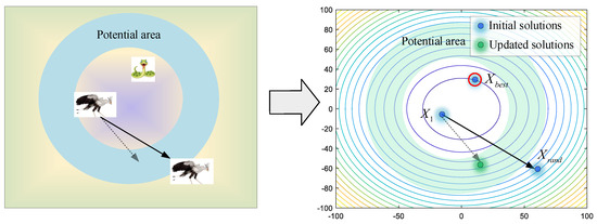
Figure 7.
The modeling process of running mode.
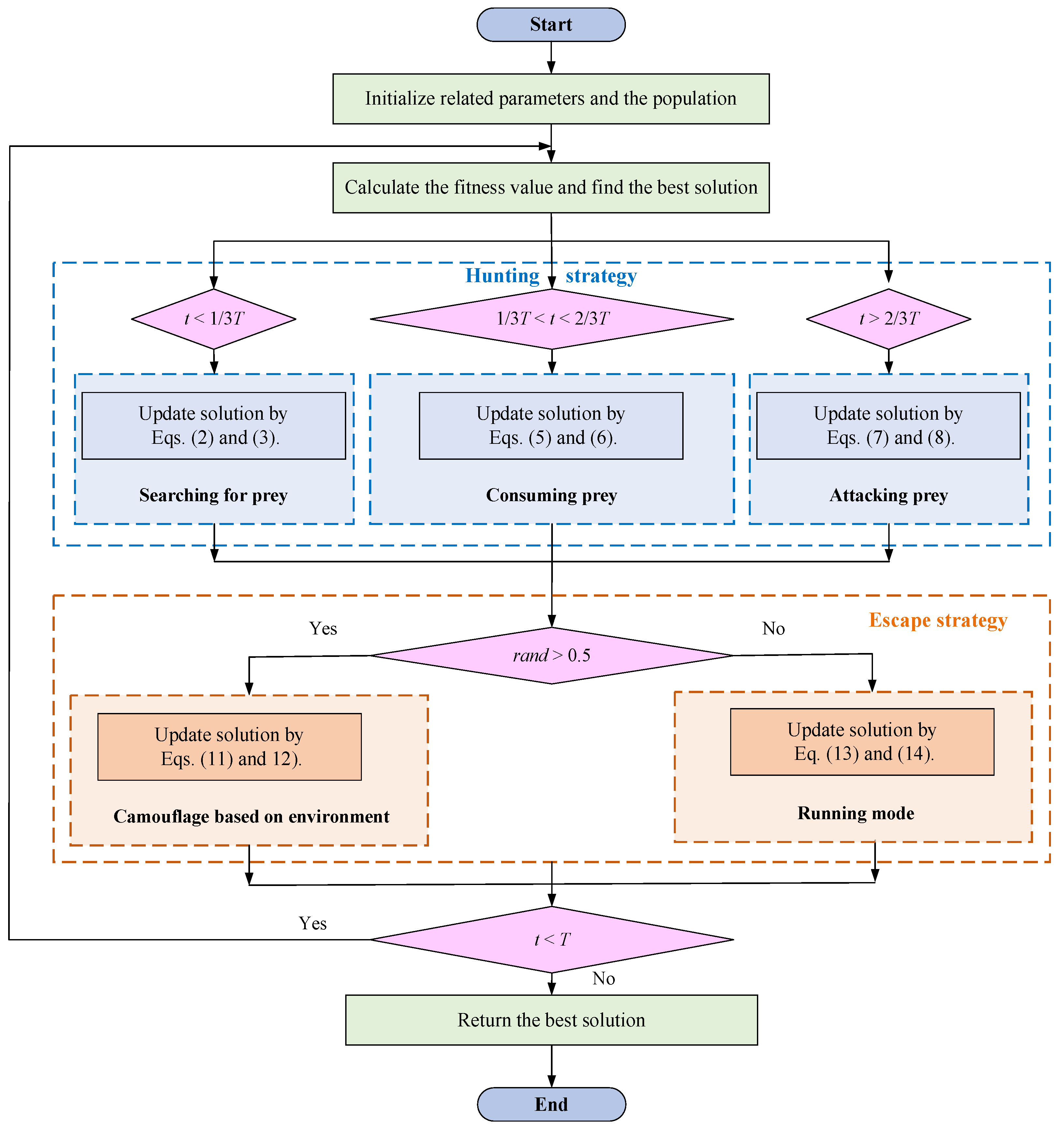
The above modes will be executed with equal probability to show the randomness of searching for the feasible area. In addition Figure 8 shows the flow chart of the original SBOA algorithm.

Figure 8.
The flowchart of the SBOA algorithm.
2.2. The Multi-Strategy Improvement Secretary Bird Optimization Algorithm
Though the SBOA has shown excellent performance in solving various test functions compared with the other 15 advanced algorithms, there are still some shortcomings in the algorithm construction, which can be further improved to obtain faster convergence and solutions with higher accuracy. The main inadequacy is reflected in the following four aspects.
- (1)
- For the whole algorithm, the global information is not fully used to adjust the position update strategy. This defect may affect the overall performance of the SBOA, which means the balance between development ability and exploration ability.
- (2)
- In the hunting stage, the attack mode of secretary birds can be further enhanced by observing the performance of the prey, which is to improve the development ability of SBOA.
- (3)
- In the escape stage, secretary birds decide how to camouflage or escape using a few simple random strategies, which may influence the ability to escape local optimums.
Aiming at the above problems, this section will introduce the appropriate strategy to construct a novel version of SBOA.
2.2.1. Feedback Regulation Mechanism
Feedback regulation mechanism is a common structural design in the biological world. It can regulate the state of the system at the next stage according to the result at the current stage after receiving the stimulus of internal and external environmental changes (Figure 9). In the field of engineering control, the PID controller is one of the most widely used automatic controllers, which is constructed by the idea of feedback regulation [34]. Among various PID methods, incremental PID control is a typical recursive algorithm, which makes the system stable by adjusting the controlled object according to the output value [35]. This kind of control method can be used in the optimization algorithm, by regarding the searching process as a system and the best fitness value in each iteration as the output value. Thus, the discrete incremental PID control is adopted to form the feedback regulation mechanism.

Figure 9.
Schematic diagram of the incremental PID control.
Firstly, the system deviations need to be defined as Equation (15).
where is the best solution in the tth iteration. To facilitate the following calculation, the deviation of the previous iteration is denoted as . The deviation of the previous two iterations is denoted as . When t = 1, let . When t > 1, . Furthermore, to reduce the space complexity, the can be calculated by
Then, the output of PID regulation in iteration t is
where r1, r2, r3 are random numbers from 0 to 1. Kp, Ki, and Kd are adjustment coefficients for the proportion, integral and differential, respectively.
Finally, the updated solutions can be calculated by the following equation:
where . is a conditioning factor to prevent the algorithm from falling into local optimum, in which and L is a Levy flight function. And r4 and r5 are random numbers from 0 to 1.
2.2.2. Golden Sinusoidal Guidance Strategy
After locking the prey, the secretary bird will start to attack the target. To enhance the success rate of capture, this section will adopt a golden sinusoidal guidance strategy to take advantage of the target’s location information [36]. In the algorithm, this strategy is useful to enhance the ability of developing local areas. For the individual i in the population, it will update its position by Equation (19).
where s1 is a random value in [0, 2π], and s2 is a random value in [0, π]. θ1 and θ2 are the coefficients obtained by the golden section, which are and , in which is defined as .
2.2.3. Cooperative Camouflage Strategy
When secretary birds feel threatened, they will first use the environment to disguise themselves. However, this kind of camouflage strategy cannot effectively avoid enemy attacks because the information exchange between populations is neglected in the original method. Thus, this section will introduce a cooperative camouflage strategy by considering the positions of different individuals. First, three different individuals need to be selected, noted as Xa, Xb, and Xc. A new solution just can be generated by Equation (20).
where r6 is a random number from 0 to 1.
2.2.4. Update Strategy Based on Cosine Similarity
When the camouflage strategy does not work, secretary birds have to run to escape enemies. Then, the key to success is how to choose the right escape direction. Generally speaking, an empty place will be the first choice to ensure sufficient space. For the individual Xi, the cosine similarity is used to measure the crowding degree to other individuals.
Firstly, construct vectors A and B by Equation (21).
where i ≠ j.
Then, calculate the similarity between Xi and Xj by Equation (22).
After comparing Xi and others, the individual with the smallest cosine similarity will be selected as the update direction, noted as Xs. A new solution can be obtained by Equation (23).
where R is a vector including random elements in [0, 1], and K is an integer, randomly toggling between 1 and 2.
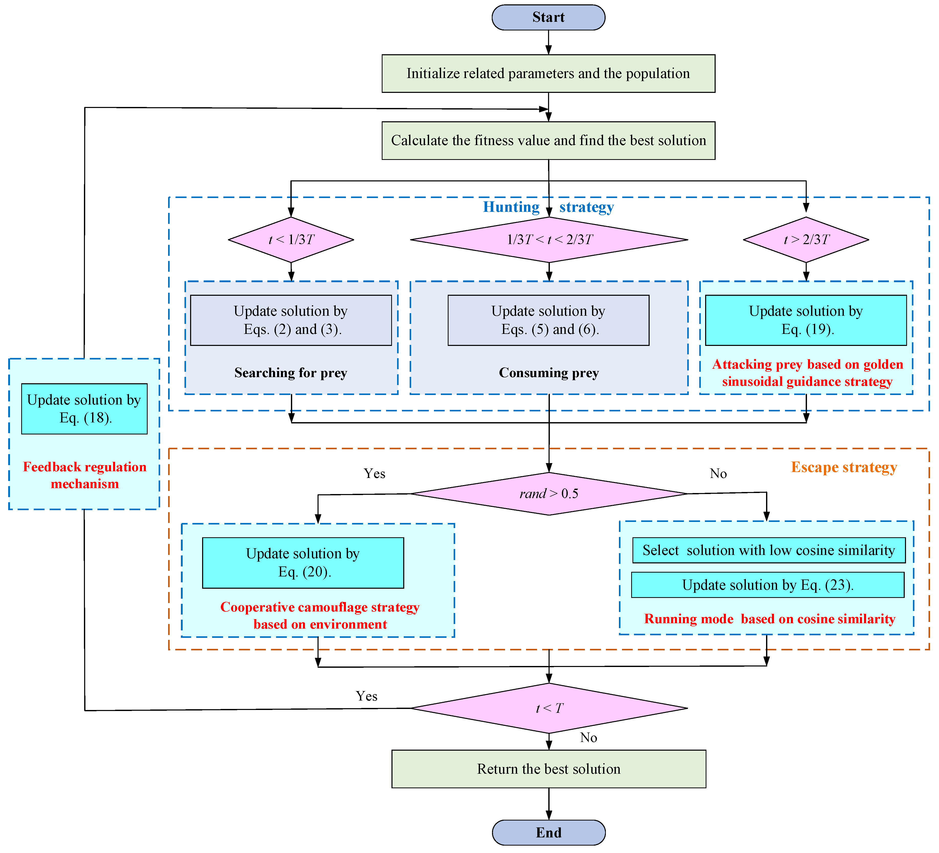
Figure 10 shows the flowchart of the MISBOA algorithm. The specific steps of the MISBOA algorithm are as follows:
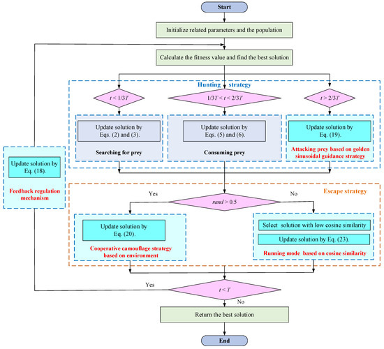
Figure 10.
The flowchart of the MISBOA algorithm.
Step 1. Initialize the related parameters and the population of secretary birds.
Step 2. Calculate the fitness value of each solution and obtain the best solution in the current population.
Step 3. According to the historical information, update solutions based on the feedback regulation mechanism in Equation (18).
Step 4. If t < T/3, secretary birds search for the prey in the hunting stage and update solutions by Equations (2) and (3).
Step 5. If T/3 < t < 2T/3, secretary birds start to consume the prey in the hunting stage and update solutions by Equations (5) and (6).
Step 6. If t > 2T/3, secretary birds are attacking the prey based on the Golden sinusoidal guidance strategy in the hunting stage and update solutions by Equation (19).
Step 7. Turn to the escape stage. If rand > 0.5, update solutions by Equation (20) based on the cooperative camouflage strategy; otherwise, update solutions by Equation (23) based on the cosine similarity.
Step 8. If t < T, turn to Step 1; otherwise, output the best solution.
2.2.5. Computational Complexity Analysis
Computational complexity is a significant metric to measure whether an optimization algorithm can be deployed and applied quickly. Based on the Big O notation, the computational complexity of basic SBOA is O(N × T × (Dim + 1)), where N, T, Dim are the population size, maximum iterations, and dimensions, respectively. For the proposed MISBOA, four introduced strategies may potentially increase the computational complexity. However, the golden sinusoidal guidance strategy, cooperative camouflage strategy, and update strategy based on cosine similarity are more effective upgraded versions of the original methods, which do not incur additional computational costs. Thus, the computational complexity is O(T × N) + O(T × N × Dim) + O(T × N × Dim), resulting in O(N × T × (2 × Dim + 1)).
3. Numerical Experiment on the Test Functions
This section will test the comprehensive ability of the proposed MISBOA algorithm. By analyzing the results of MISBOA and other selected algorithms in solving test functions of the CEC2022 test suite, the effectiveness of the introduced strategy will be discussed.
3.1. Test Functions and Parameter Setting
For the objectivity and rationality of the experiment, it is inevitable to select other typical intelligent optimization algorithms as the control group. In this paper, other 8 popular algorithms are selected, which are the original SBOA [33], the golden jackal optimization algorithm (GJO) [37], the particle swarm optimization algorithm (PSO) [38], the PID-based search algorithm (PSA) [35], the quadratic interpolation optimization algorithm (QIO) [39], the Newton-Raphson-based optimizer (NRBO) [40], and the sand cat swarm optimization algorithm (SCSO) [41]. The parameters of the other metaheuristic algorithms are listed in Table 1.

Table 1.
Parameters of the selected algorithms.
For the CEC2022 test suite, there are 12 test functions, including unimodal functions, basic functions, hybrid functions, and composition functions. The dimension of test functions can be set as 10 or 20 [42]. Thus, for comprehensiveness and reliability, this section will test MISBOA and other comparison algorithms on the 12 test functions of 10 and 20 dimensions.
For the experiment conditions, the size of the initial population for all algorithms is set to 100, and the maximum iteration time is set to 1000. Then, the results of various algorithms will be recorded after 30 independent runs to avoid the influence of chance factors. The average value (Ave) and the standard deviation of the obtained 30 results will be used as the main indexes to evaluate the quality of various algorithms. Another index rank is determined by arranging the average values in ascending order. The smaller ranking result represents better performance. Average time cost (in seconds) for each function after 30 runs is also recorded to reflect the computational complexity of various algorithms.
3.2. Analysis and Discussion of the Results on CEC 2022 with 10 Dimensions
Firstly, the solving results of CEC 2022 with 10 dimensions are summarized in Table 2. The data marked in bold means the best results among all algorithms for the according evaluation index. Results show that the constructed MISBOA algorithm has the best performance for 6 test functions, followed by SBOA and QIO, which perform best on 1 and 4 test functions. Comparing the MISBOA and the basic SBOA, MISBOA can keep advantage over SBOA on 10 test functions, except for CEC09 and CEC12. For CEC03 and CEC05, the MISBOA can achieve the theoretical optimums after each run. However, the SBOA can only obtain the ideal results in a few experiments, which leads to a larger standard deviation. For the QIO algorithm, it can also rank first on 4 test functions, but its performance is not stable for all functions with various characters. For example, QIO only ranks fourth on CEC01, CEC02, CEC03, and CEC08 and ranks eighth on CEC12. The improved MISBOA ranks in the top three on all functions. It illustrates the introduction of multiple strategies effectively balances the capacities of exploration and development, further having stronger searching ability for various optimization problems. Based on the final ranking results, the performances of MISBOA and other algorithms are ranked as MISBOA > SBOA > QIO > PSA > PSO > PSOBKA > NRBO > SCSO > GJO. For time cost, the MISBOA inevitably consumes slightly more time compared to the original SBOA, which is consistent with the results of the complexity analysis. However, facing the NRBO and SCSO, the MISBOA emerges as the winner and competes evenly with the QIO algorithm. That is, the proposed MISBOA achieves higher solving accuracy while simultaneously minimizing increases in time costs as much as possible.

Table 2.
Results of different algorithms on CEC2022 functions with 10 dimensions.
To support the above conclusions from statistical knowledge, Table 3 lists the p-value of the Wilcoxon rank sum test (WRST) between the proposed MISBOA and other algorithms. If the MISOBA performs better than another algorithm and the p-value is less than 0.05, it can illustrate the MISOBA is obviously superior to the comparison algorithm, noted ‘+’. Otherwise, if MISOBA performs worse than another algorithm and the p-value is less than 0.05, it is noted as ‘−’. If the p-value is over 0.05, there is no statistically significant difference between the two algorithms. From Table 3, compared with the SBOA, the improved algorithm gets the statistical advantage on 9 test functions and is obviously inferior to the original version on CEC12. For QIO, the MISBOA performs greatly better on 7 test functions and worse on 4 test functions. For BKA, GJO, PSO, NRBO, and SCSO, the advantages of all test functions of MISBOA can be supported by WRST.

Table 3.
The p-value of WRST between the MISBOA and other algorithms on CEC2022 with 10 dimensions.
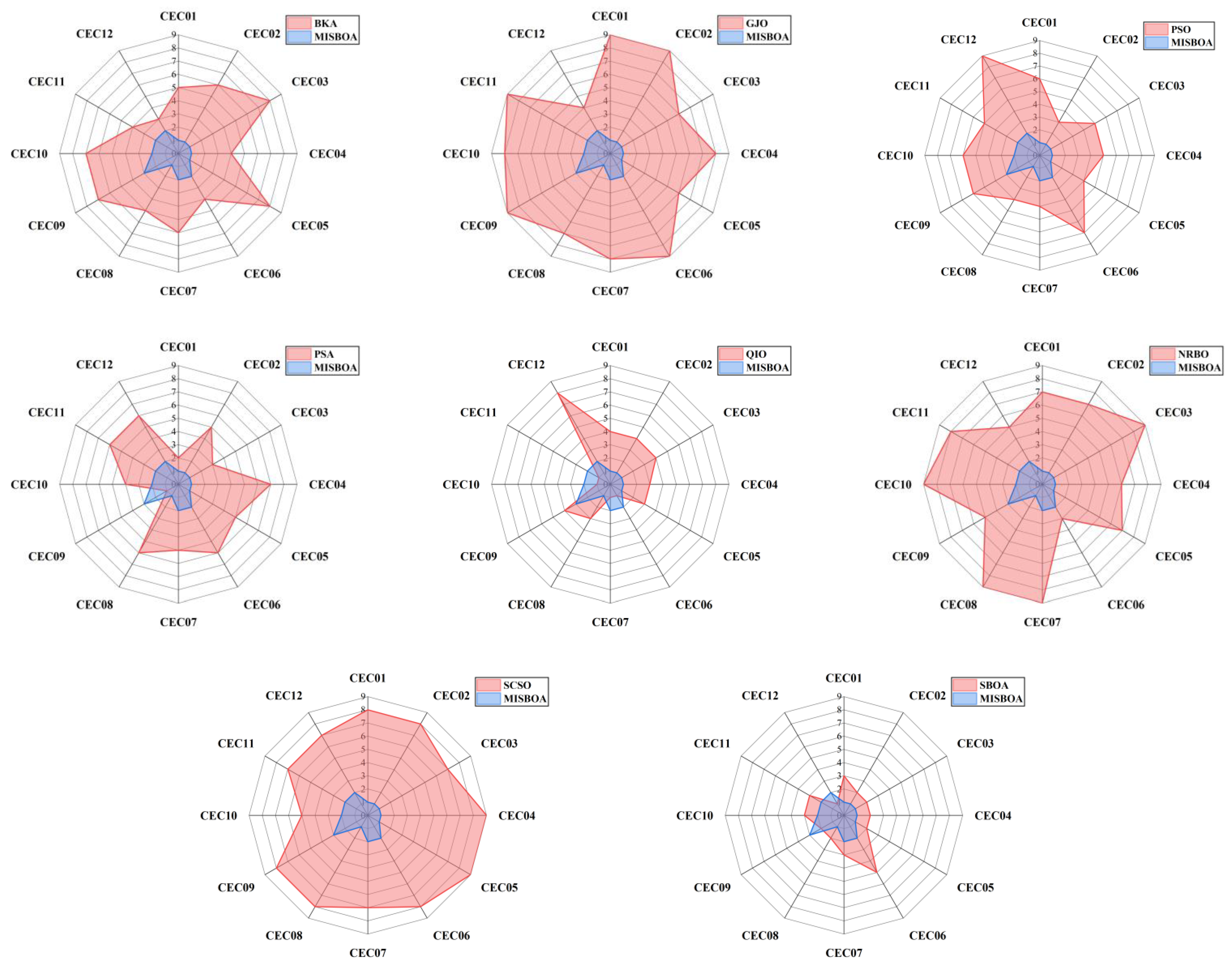
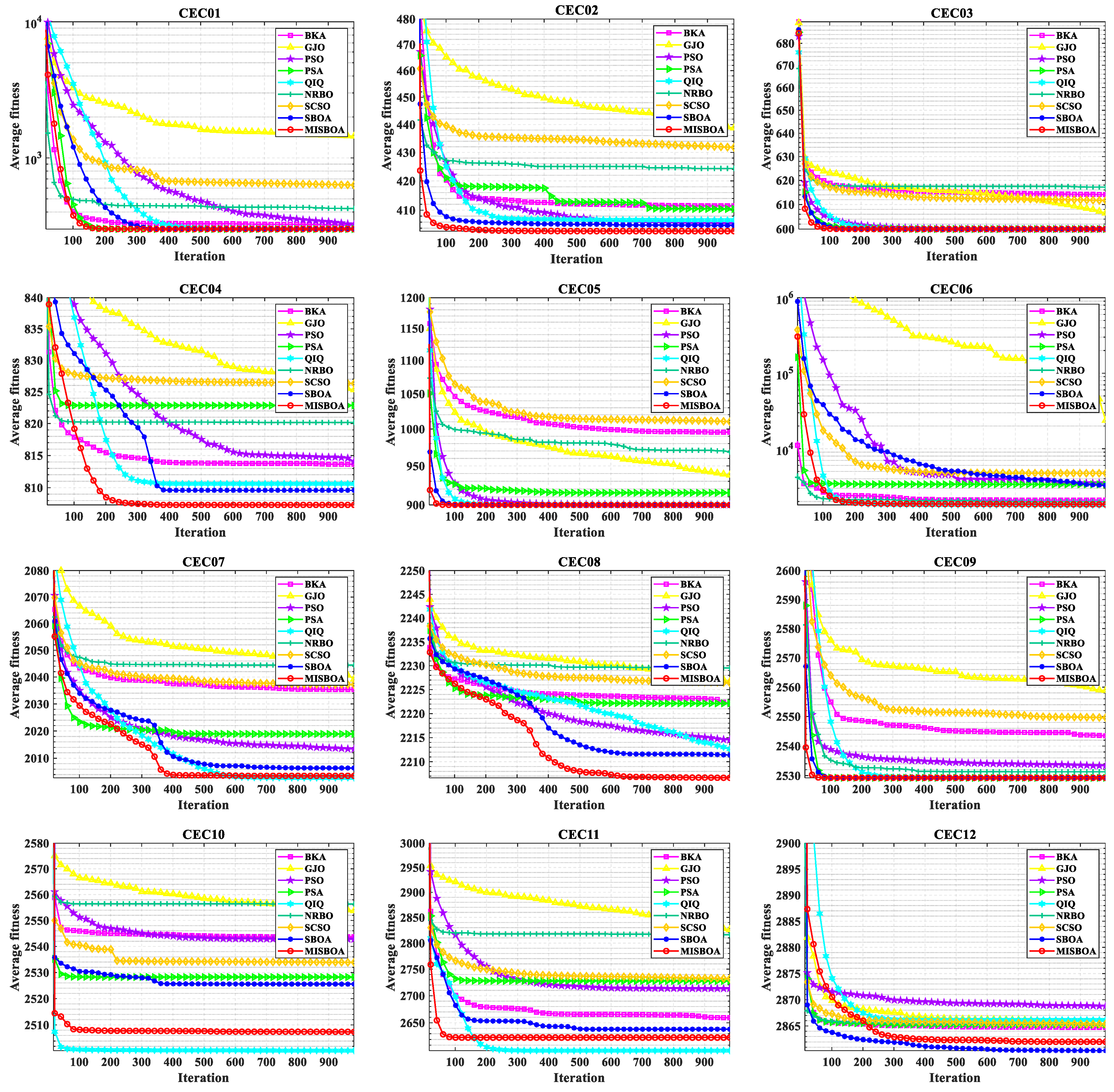
Figure 11 plots radar comparison maps between MISBOA and other algorithms on CEC2022 with 10 dimensions. A smaller radar coverage area means the algorithm has a more stable solving ability for various test functions in CEC2022. Compared with BKA, GJO, PSO, NRBO, and SCSO, the MISBOA takes advantage of all functions. For PSA, QIO, and SBOA, though the MISBOA cannot rank first on a few functions, its comprehensive performance is still excellent. The average iterative curves of different algorithms after 30 runs are shown in Figure 12. From the curves, convergence rate and accuracy can be visually observed and analyzed. Compared with the original SBOA, the convergence rate of the proposed algorithm is obviously faster than SBOA on CEC01, CEC02, CEC04, CEC06, CEC07, CEC08, CEC10, and CEC11 during the whole searching process. This kind of advantage comes from the comprehensive impact of multiple strategies. The introduction of the feedback regulation mechanism can constantly adjust updated strategies based on historical information to ensure the quality of the entire population. The golden sinusoidal guidance strategy also improves the local development capacity, leading to individuals converging to better solutions with faster speed. Thus, at the early stage, the curves of MISBOA fall faster. At the later stage, the cooperative camouflage strategy and update strategy based on cosine similarity play roles in improving the ability to keep the population diversity and avoiding the local optimums. Compared with the QIO, though the MISBOA is at a disadvantage on CEC10 and CEC11, the performance of the QIO on other test functions lacks stability.
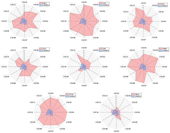
Figure 11.
The radar comparison maps between MISBOA and other algorithms on CEC2022 with 10 dimensions.
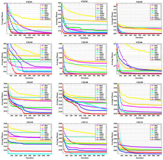
Figure 12.
The average iterative curves of different algorithms on CEC2022 with 10 dimensions.
3.3. Analysis and Discussion of the Results on CEC 2022 with 20 Dimensions
Then, to verify the scalability of the MISBOA algorithm, this section compares it with other selected algorithms on test functions in CEC2022 with 20 dimensions. With the increase of decision variables, the fast convergence ability of algorithms in the feasible space is further required. After 30 runs, the data is collected in Table 4. Except for CEC 04 and CEC10, the MISBOA ranks first on the rest 10 test functions. Compared with the results on CEC2022 functions with 20 dimensions, the advantages of MISBOA are further expanded. It illustrates the performance of MISBOA is still stable with the increase of dimensions. For the original SBOA, facing more decision variables, it ranks first on only 1 test function. That is, without the improved strategies, the basic algorithm cannot effectively search for solutions with higher accuracy. The performance of the QIO algorithm is similar, ranking first only on CEC10. Thus, the application of feedback regulation mechanisms, golden sinusoidal guidance strategies, cooperative camouflage strategies, and update strategies based on cosine similarity is a helpful approach to balancing the abilities of exploration and development. With increased dimensions, all algorithms incur higher time costs. However, the changes of MISBOA and SBOA are minimal compared to QIO, NRBO, and SCSO. That is, the structure of the MISBOA algorithm effectively mitigates the increase in time costs caused by growth in problem dimensions.

Table 4.
Results of different algorithms on CEC2022 functions with 20 dimensions.
Table 5 includes the p-value of WRST between MISBOA and other algorithms on CEC2022 with 20 dimensions. With the increase in dimensions, the difference between MISBOA and other algorithms is further revealed. For example, compared with the SBOA, MISBOA performs significantly better on 10 test functions under the conditions of 20 dimensions, more than that of 10 dimensions. This phenomenon is even more obvious when the MISBOA is compared with the QIO. The results of WRST prove that the MISBOA is obviously superior to QIO on 9 test functions and performs worse on only 1 test function. This result illustrates that the MISBOA is also effective when the dimension of problems is increased, while the performance of QIO is greatly affected. The radar comparison maps between MISBOA and others on CEC2022 with 20 dimensions in Figure 13 also prove that conclusion.

Table 5.
The p-value of WRST between the MISBOA and other algorithms on CEC2022 with 20 dimensions.
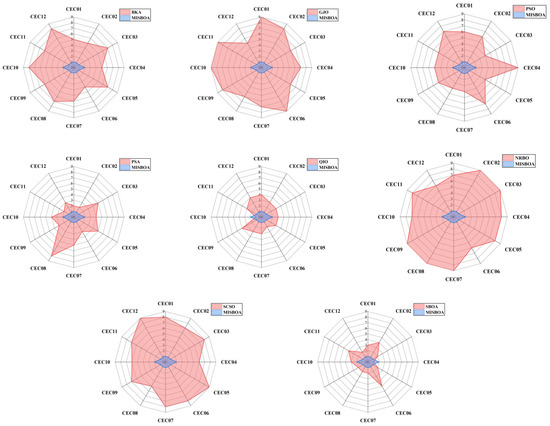
Figure 13.
The radar comparison maps between MISBOA and other algorithms on CEC2022 with 20 dimensions.
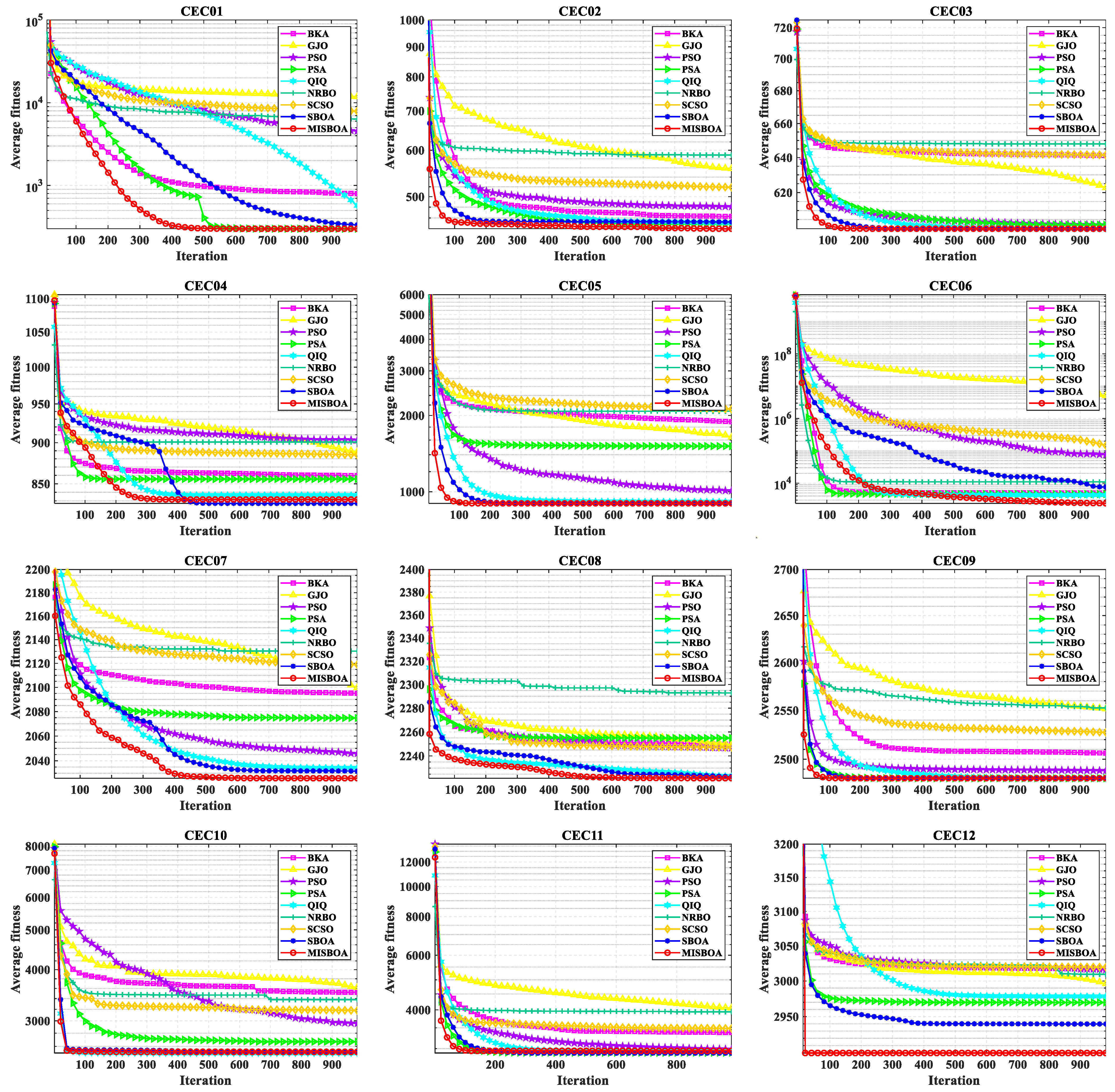
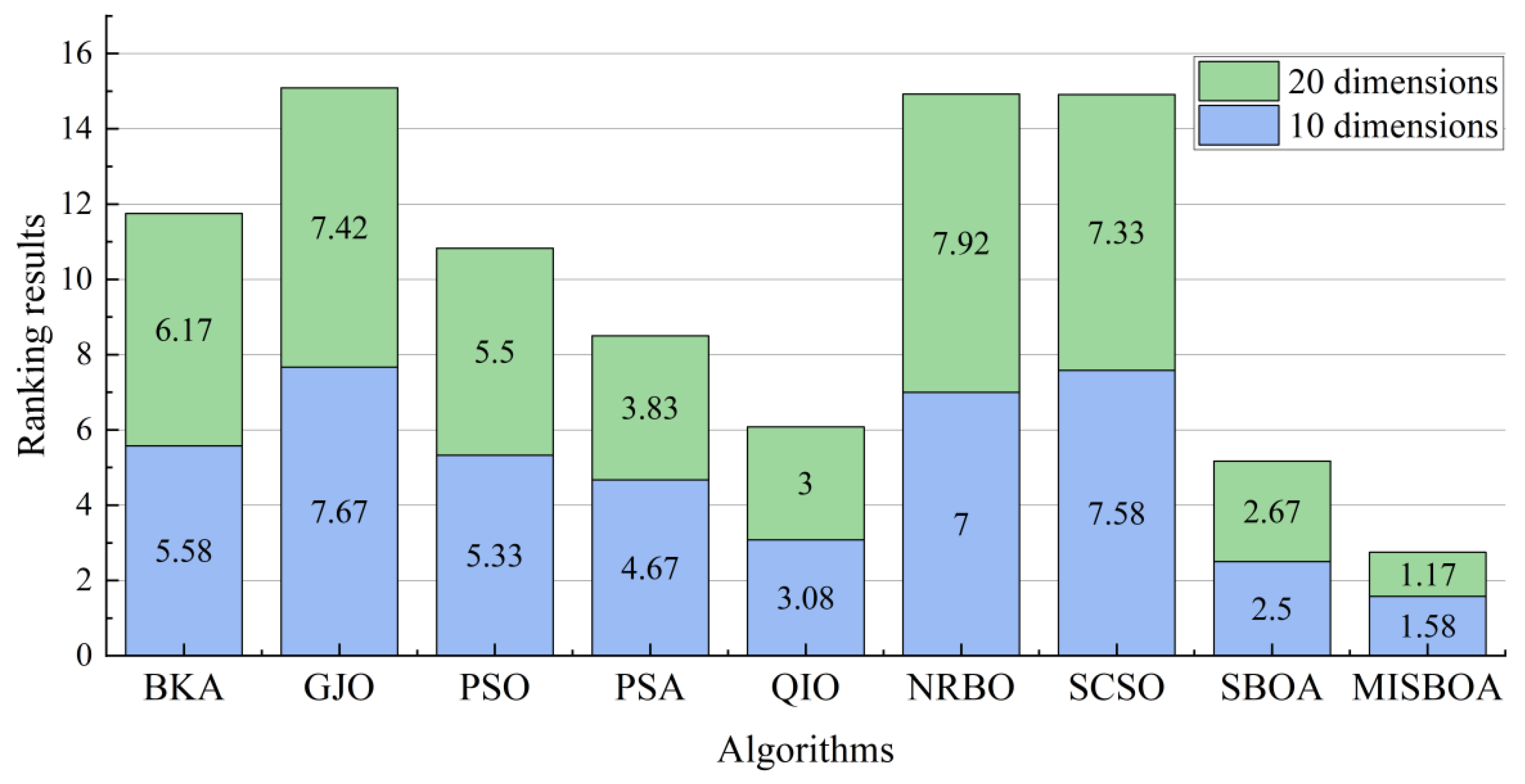
Figure 14 plots the average iterative curves of different algorithms on CEC2022 with 20 dimensions. It can be observed that the advantage of MISBOA in convergence speed is established in the beginning for all algorithms except for CEC06. It illustrates the value of the feedback regulation mechanism and golden sinusoidal guidance strategy. By referring to the historical information and the best solution in current, the whole population can quickly be close to better solutions. Meanwhile, for CEC06, when other algorithms cannot continue to find better solutions in the later stage, the iterative curve of MISBOA is still falling to explore feasible solutions with higher precision. It is the value of cooperative camouflage strategy and update strategy based on cosine similarity. By using the information of random individuals and individuals with small cosine similarity, the diversity of the population can be maintained to avoid local optimums. Figure 15 is the statistical results of ranking on CEC2022 with 10 and 20 dimensions. For MISBOA, it has the smallest ranking result for test functions with 10 and 20 dimensions, respectively. With the increase of decision variables, the average rank of MISBOA is smaller, meaning its competitiveness, universality, and stability for complex optimization algorithms with different characters.
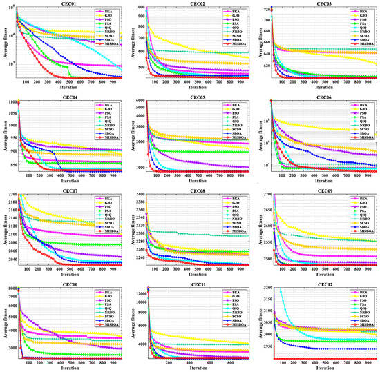
Figure 14.
The average iterative curves of different algorithms on CEC2022 with 20 dimensions.

Figure 15.
The statistical results of ranking on CEC2022 with 10 and 20 dimensions.
4. The Application for Real-World Optimization Problems
In addition, the test functions of CEC2022, the performances of novel algorithms must be verified in solving real-world optimization problems [43]. In this section, five typical engineering optimization problems are used to test the abilities of MISBOA and other algorithms, firstly [44]. Then, the MISBOA is employed to solve a shape optimization problem of combined curves with multiple shape parameters. Based on the 8 comparison algorithms in Section 4, four popular algorithms widely used in practice are added, which are Harris hawks optimization (HHO) [45], walrus optimizer (WO) [46], grey wolf optimization algorithm (GWO) [14], and whale optimization algorithm (WOA) [47].
4.1. Engineering Optimization Problems
The results will be recorded after 10 independent runs for each algorithm. For all problems, the size of the population and maximum iteration are 50 and 300, respectively. To fairly measure the performance of different algorithms, the best value, average value, worst value, and standard deviation (Std) results after 10 runs will be calculated. Meanwhile, based on the average value, the ranking result for each algorithm can be determined to illustrate its combination performance.
4.1.1. Step-Cone Pulley Design Problem
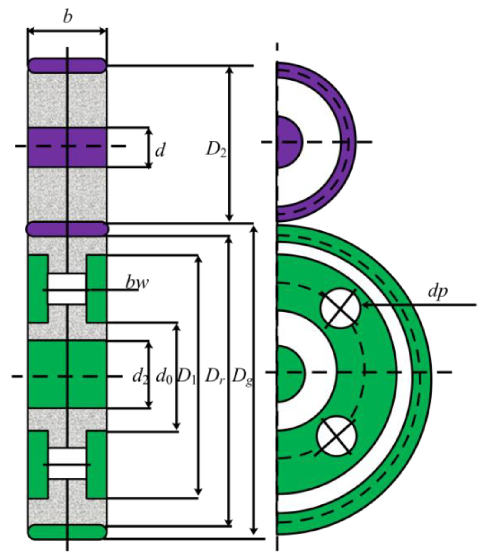
The main goal of this problem is to minimize the weight of the four stepped cone pulleys by adjusting five key variables, which are the diameter of each pulley (d1, d2, d3, d4) and the width of the pulley (w). As shown in Figure 16, the system contains 11 nonlinear constraints to ensure that the transmitted power must be at 0.75 hp. Its mathematical model is defined in Equation (24).
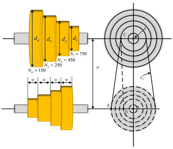
Figure 16.
The construction of step-cone pulley design.
Table 6 summarizes the results of MISBOA and others for the step-cone pulley design problem. Observing the index of best value, the MISBOA and SBOA obtain the same fitness values, which are better than others. However, for the index of worst value, the SBOA is inferior to MISBOA, meaning the stability of MISBOA is enhanced by introducing multiple effective, improved strategies. Thus, for the final ranking results, the proposed MISBOA performs excellently. Smaller Std also supports the conclusion that the MISBOA is not easy to be affected by accidental factors when solving engineering optimization problems. Table 7 lists the best variables obtained by various algorithms for this design problem according to the best fitness value in Table 6.

Table 6.
Results of various algorithms for the step-cone pulley design problem.

Table 7.
The best variables of various algorithms for the step-cone pulley design problem.
4.1.2. Planetary Gear Train Design Problem
The main aim of the planetary gear train design optimization problem is to minimize the maximum error of the transmission ratio used in automobiles. To achieve the target, 9 variables are needed to be adjusted, as shown in Figure 17. In these variables, 6 integer variables (N1, N2, N3, N4, N5, N6) represent the number of the gear teeth, and 3 discrete variables represent the number of gear modulus (m1, m2) and the number of planetary gear teeth (p). The established model of the planetary gear train design system is shown in Equation (25).

Figure 17.
The construction of the planetary gear train design.
In Table 8, the solving results of MISBOA and others are shown for the design problem of the planetary gear train design. For the index of best value, the BKA and WOA perform better than the MISBOA, but the MISBOA’s average value and Std have obvious advantages, which lead to the better ranking result. It illustrates the superior comprehensive performance of the MISBOA. It is not reliable if an algorithm can achieve better solutions for only several runs but perform poorly for lots of experiments. Thus, especially for engineering optimization problems, the MISBOA is competitive due to its stronger stability. Table 9 shows the best variables of selected algorithms according to the best solution.

Table 8.
Results of various algorithms for the planetary gear train design problem.

Table 9.
The best variables of various algorithms for the planetary gear train design problem.
4.1.3. Robot Gripper Design Problem
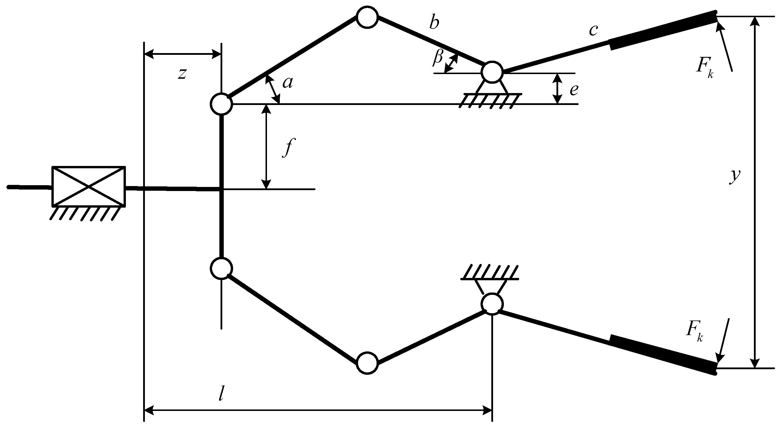
The problem of robot gripper is a popular optimization problem in mechanical structure engineering. As shown in Figure 18, this system consists of 6 factors, which are connecting rod length, geometric angle between connecting rods, vertical displacement, clamping pressure, actuator displacement of the robotic gripper, and horizontal displacement. 7 key parameters influence the performance of the system, which are three links (a, b, c), the vertical distance between the first robotic arm node and the actuator end f, the vertical displacement of the links e, the geometric angle between the second and third links d, and the horizontal distance between the actuator end and the links node l. By adjusting these key parameters, the minimum value of the difference between the minimum and maximum force needs to be obtained. This problem can be described by Equation (26).

Figure 18.
The construction of the robot gripper design.
Table 10 provides the results of various algorithms for the robot gripper design problem. For this complex system, the MISBOA achieves the advantages on all four measure indexes. Thus, the MISBOA can be regarded as an effective and reliable approach to solve the design problem of the robot gripper. This kind of preponderance comes from the suitable and reasonable combination of various improved strategies, which leads to better performance in balancing the abilities between exploration and development. Table 11 shows the best control parameters in the robot gripper system according to the best fitness value.

Table 10.
Results of various algorithms for the robot gripper design problem.

Table 11.
The best variables of various algorithms for the robot gripper design problem.
4.1.4. Four-Stage Gearbox Design Problem
In this problem, researchers must reduce the total weight of the gearbox system by optimizing 22 key variables, as shown in Figure 19. These parameters can be divided into four classes, including the positions of the gears, and pinions, the thickness of the blanks, and the number of teeth. Meanwhile, 86 constraint conditions need to be satisfied, increasing the difficulty of this problem. These requirements involve the contact ratio, pitch, strength of the gears, assembly of gears, kinematics, and size of the gears. The model can be represented by the following:
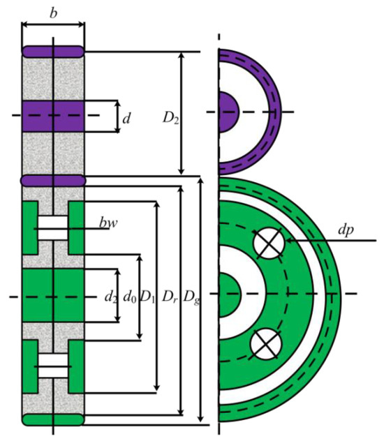
Figure 19.
The construction of the four-stage gearbox design problem.
Table 12 includes the solving results of all algorithms for the four-stage gearbox design problem. From the results, it can be noticed that the performance of different algorithms varies a lot due to the increase of variables and the introduction of lots of constraints. For example, though the SBOA achieves the best value after 10 runs, its average value is poor compared with the MISBOA. Compared with other algorithms, the advantage of MISBOA on the index of average value is further expanded. Thus, the MISBOA is a suitable tool for this complex problem. Table 13 shows the best variables according to the best fitness value of each algorithm.

Table 12.
Results of various algorithms for the four-stage gearbox design problem.

Table 13.
The best variables of various algorithms for the four-stage gearbox design problem.
4.1.5. Traveling Salesman Problem
The traveling salesman problem (TSP) is a well-known combinatorial optimization problem. In this problem, each salesman needs to find a path in a certain number of cities to make the total length of the shortest path. Meanwhile, the planned path has to satisfy the requirement, which passes through each city once and only once and finally returns to the starting point. TSP is widely applied for practical applications, such as logistics, transportation, and other fields. Because the candidate solutions to this problem are the full permutation of all cities, the difficulty of this problem will increase dramatically with the increase in the number of cities.
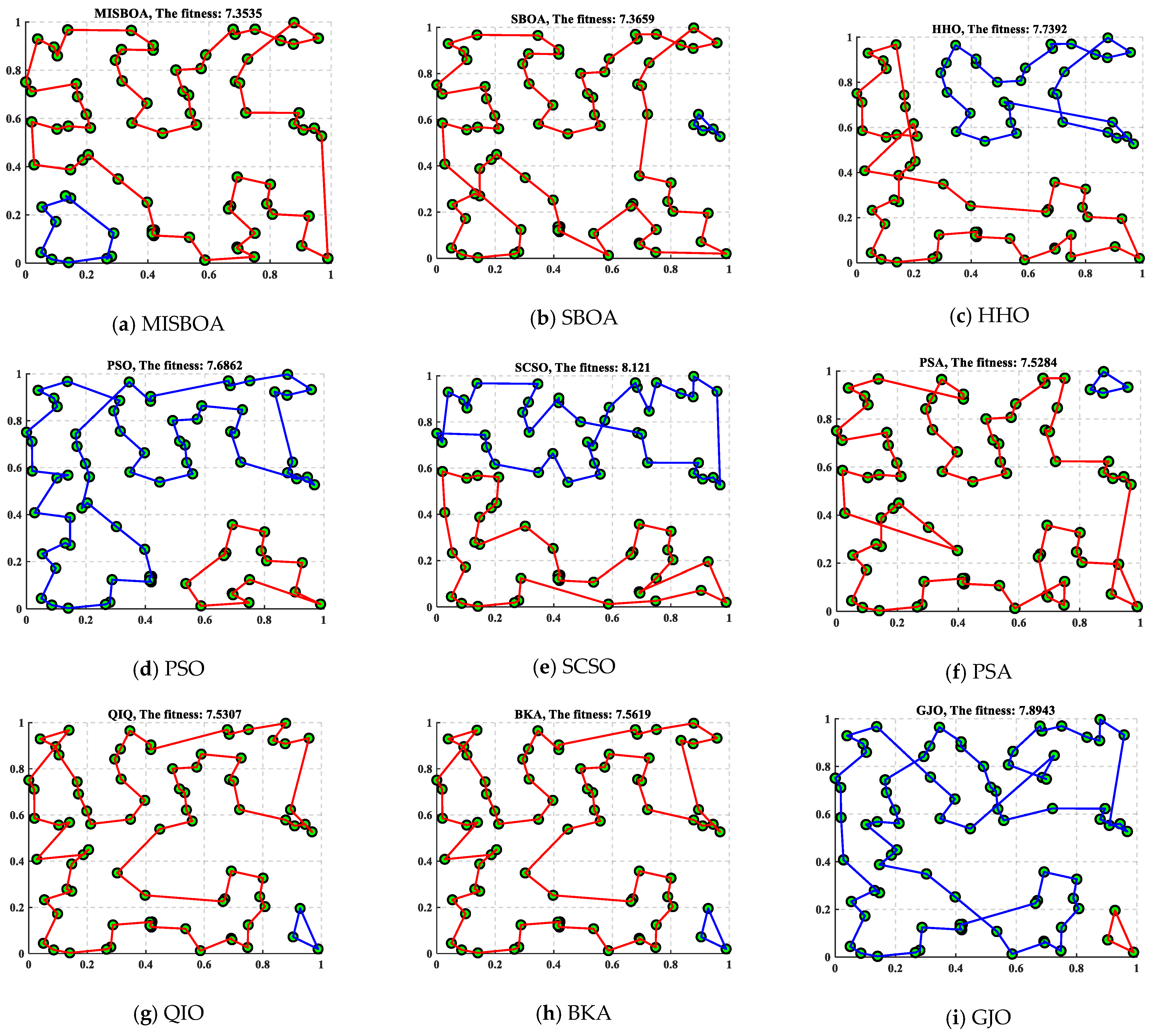
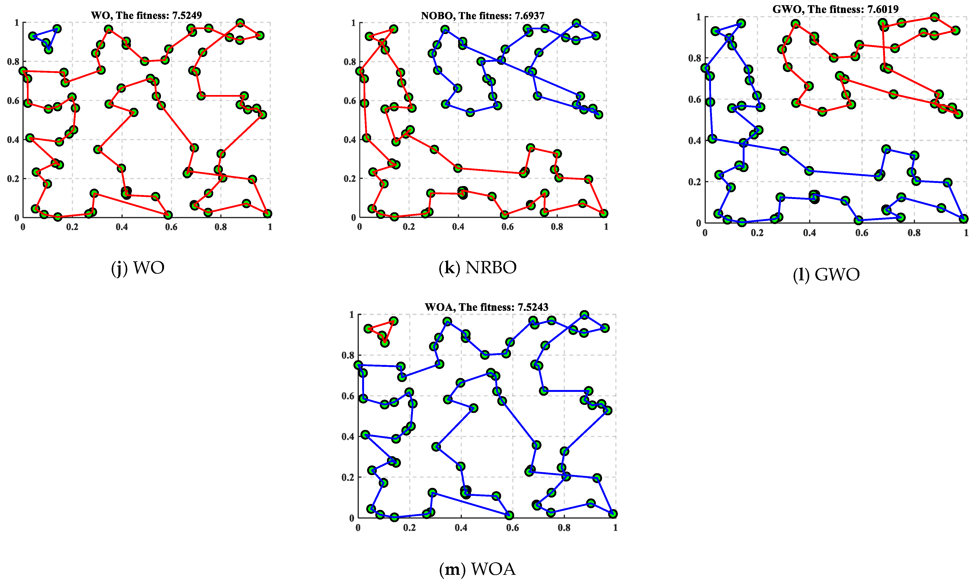
In this case, there are 80 randomly generated cities and 2 traveling salesmen. Table 14 includes the results obtained by MISBOA and others for the TSP with 80 cities and 2 traveling salesmen. For the indexes of the best, average, and standard, the MISBOA ranks first. That is, for complex problems with lots of variables, the MISBOA can reasonably search for the feasible space with the suitable strategies in different stages. For the original SBOA, the lack of more effective searching strategies leads to its worse overall performance compared with the MISBOA. Figure 20 plots the best routes for travel salesman obtained by different algorithms and their convergence curves and the box plots. Comparing Figure 20a,b, the number of cities visited by the two salesmen is not evenly balanced. Compared with other solutions, the route of MISBOA is more reasonable, which avoids additional consumption. However, routes based on other algorithms are wound together, leading to longer total distance.

Table 14.
The results of various algorithms for TSP.
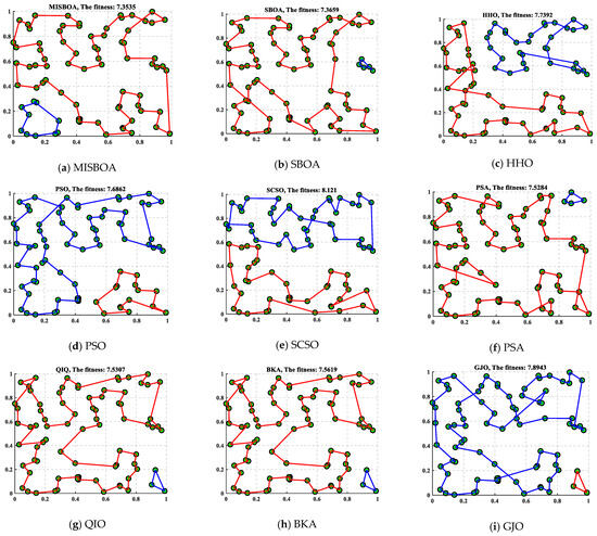

Figure 20.
The best results for TSP with 80 cities and 2 traveling salesman.
4.2. Shape Optimization Problems of Combined Curves
In the field of practical engineering applications, it is of great significance to generate a smooth curve that can pass through all given data points by the interpolation approach [48]. In this section, the energy of the combined quartic generalized Ball interpolation (CQGBI) curve is studied and optimized.
The CQGBI curve is constructed by combing several quartic curves. For the given data points , a CQGBI curve can be obtained, as shown in Equation (28) [49].
where
in which are the shape parameters and can be adjusted.
Hence, it is necessary to select more suitable parameters to maintain the smoothness of the obtained combined curve. Here, the curvature variation energy is used to measure the smoothness of the CQGBI curve, which is [50].
where is the curve of the j-th section of the CQGBI curve.
After further calculation, Equation (30) can be represented by
Combined Equation (30) and Equation (31), we can obtain
where , , , , .
Then, by regarding the total energy of the whole CQGBI curve, the optimization model can be established by Equation (33).
That is, for a CQGBI curve with n + 1 data points, there are 2n parameters that need to be optimized. Here, the shape optimization problem of wind-driven generator blades is studied. As shown in Figure 21, as a core component of wind power generation systems, the shape of wind-driven generator blades will significantly affect the efficiency of power generation. Thus, the MISBOA and other algorithms are used to select the most suitable parameters to reduce the energy of the CQGBI curve, which describes the shape of a wind-driven generator blade.
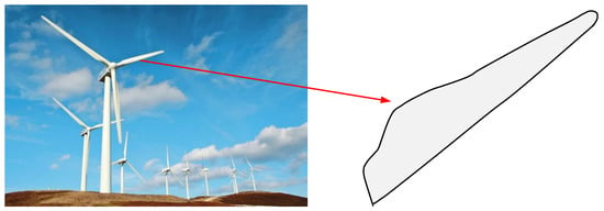
Figure 21.
The shape of wind-driven generator blades.
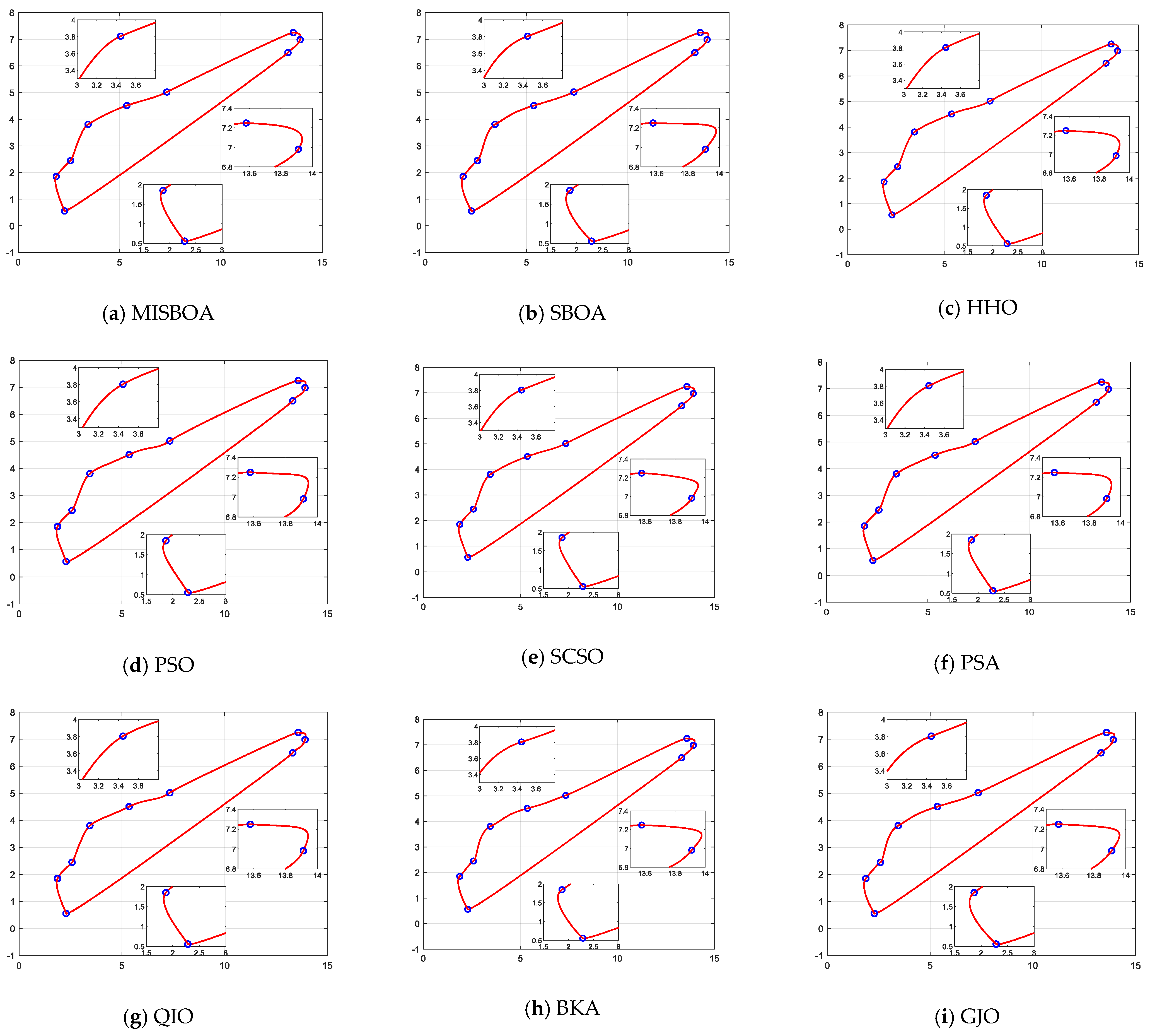
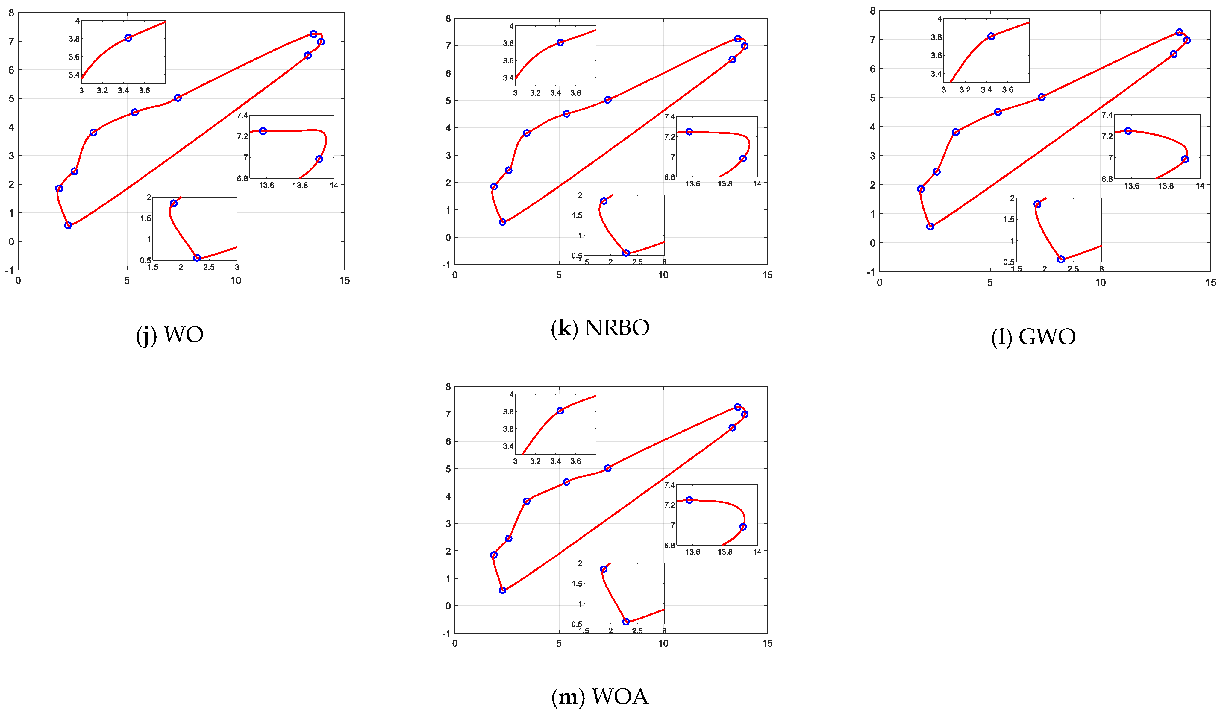
After 10 times running, the results of various algorithms for the shape optimization problem of wind-driven generator blades are listed in Table 15. From the summarized data, the MISBOA finally ranks first due to its excellent performance on the four measure indexes. Especially for the standard deviation, the MISBOA is significantly superior to other algorithms. That is, it even can achieve similar solutions with higher accuracy for each running, meaning the ability to get better results in fewer execution times. For the original SBOA, its performance is severely affected, only ranking fifth. The QIO and HHO obtain the same best value but have poor comprehensive performance due to the larger average value. Based on the best solution, the best designs for wind-driven generator blades are plotted in Figure 22. Local enlargements of some key sites are also drawn. For the solutions with larger fitness values, curves at corners are not smooth and will affect power generation efficiency, such as Figure 22d,i,l. For the MISBOA, the CQGBI curve is smoother to reduce unnecessary wastage.

Table 15.
The results of various algorithms for shape optimization problems of combined curves.
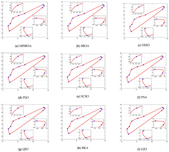
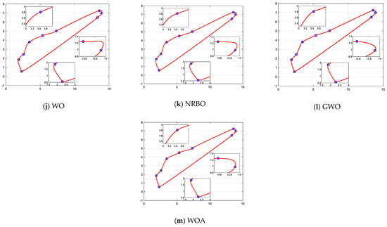
Figure 22.
The best design for wind-driven generator blades according to the best solutions of various algorithms.
5. Conclusions and Future Work
Aiming at the defects of the original SBOA algorithm, this paper proposed an improved version by introducing four specific strategies. Firstly, a feedback regulation mechanism based on incremental PID control is applied. It aims to keep higher searching effectiveness by updating the whole population according to the output value. In the hunting stage, to enhance the success rate of capture, a golden sinusoidal guidance strategy is employed. Meanwhile, to keep the population, diversity, a cooperative camouflage strategy, and an update strategy based on cosine similarity are introduced into the escaping stage.
According to the obtained results in solving test functions of the CEC2020 suite. When the dimension is 10, the MISBOA can rank firstly on 6 functions, while the SBOA can rank firstly only on 1 and 4 functions. Meanwhile, the comprehensive performance of each algorithm on different functions is compared by radar map. Though the final rank of QIO is the second, it ranks fourth on 4 functions and only ranks eighth on CEC12, meaning poorer stability than MISBOA. The worst rank of MISBOA is third on only one function. When the dimension is increased to 20, the advantage of MISBOA is more obvious. It ranks first on the rest 10 test functions, accounting for 83.33% of the total. The original SBOA and QIO algorithms rank first on only 1 test function. This difference illustrates the introduction of improvement strategies that effectively enhance the searching accuracy and stability of MISBOA for various problems. From the convergence curves, due to the effect of the feedback regulation mechanism and golden sinusoidal guidance strategy, the MISBOA can quickly approach better solutions. In the later searching process, it also can keep staying ahead because two strategies can help MISBOA escape local optimums. For five real-world optimization problems, the MISBOA also has the best performance on the fitness values, indicating stronger searching ability with higher accuracy and stability. Finally, when it is used to solve the shape optimization problem of the CQGBI curve, the shape can be designed to be smoother according to the obtained parameters based on MISBOA to improve power generation efficiency.
In the future, the practical application of the MISBOA algorithm will be further explored. Meanwhile, whether the improved strategy adopted in this paper will have a positive impact on other original algorithms is also a problem that needs to be studied.
Author Contributions
Conceptualization, S.Q., J.L. and G.H.; Methodology, S.Q., J.L., X.B. and G.H.; Software, S.Q. and X.B.; Validation, J.L. and X.B.; Formal analysis, J.L.; Investigation, S.Q., J.L., X.B. and G.H.; Resources, J.L. and G.H.; Data curation, S.Q. and X.B.; Writing—original draft, S.Q., J.L., X.B. and G.H.; Writing—review & editing, S.Q., J.L., X.B. and G.H.; Visualization, S.Q. and X.B.; Supervision, G.H.; Project administration, S.Q., J.L. and G.H.; Funding acquisition, J.L. All authors have read and agreed to the published version of the manuscript.
Funding
This work is supported by Shaanxi Key Research and Development General Project (2024GX-YBXM-529); Shaanxi Province Art and Science Planning Project (2023HZ1758); Shaanxi Provincial Social Science Fund Project (2023J005); Research Project on Experimental Teaching and Teaching Laboratory Construction of the Ministry of Education (SYJX2024-023).
Institutional Review Board Statement
Not applicable.
Data Availability Statement
All data generated or analyzed during the study are included in this published article.
Conflicts of Interest
The authors declare no conflicts of interest.
References
- Li, W.; Wang, G.-G.; Gandomi, A.H. A survey of learning-based intelligent optimization algorithms. Arch. Comput. Methods Eng. 2021, 28, 3781–3799. [Google Scholar] [CrossRef]
- Tsai, S.C.; Yeh, Y.; Wang, H.; Chou, T.C. Efficient optimization in stochastic production planning problems with product substitution. Comput. Oper. Res. 2024, 164, 106544. [Google Scholar] [CrossRef]
- Li, Q.; Guo, L. Nature-inspired metaheuristic optimization algorithms for urban transit routing problem. Eng. Res. Express 2023, 5, 015040. [Google Scholar] [CrossRef]
- Hu, G.; Gong, C.; Li, X.; Xu, Z. CGKOA: An enhanced Kepler optimization algorithm for multi-domain optimization problems. Comput. Methods Appl. Mech. Eng. 2024, 425, 116964. [Google Scholar] [CrossRef]
- Truong, D.-N.; Chou, J.-S. Fuzzy adaptive forensic-based investigation algorithm for optimizing frequency-constrained structural dome design. Math. Comput. Simul. 2023, 210, 473–531. [Google Scholar] [CrossRef]
- Hu, G.; Huang, F.; Seyyedabbasi, A.; Wei, G. Enhanced multi-strategy bottlenose dolphin optimizer for UAVs path planning. Appl. Math. Model. 2024, 130, 243–271. [Google Scholar] [CrossRef]
- Younis, H.B.; Moosavi, S.K.; Zafar, M.H.; Hadi, S.F.; Mansoor, M. Feature selection based on dataset variance optimization using Whale Optimization Algorithm (WOA). In Handbook of Whale Optimization Algorithm; Academic Press: Cambridge, MA, USA, 2024; pp. 547–565. [Google Scholar]
- Hu, G.; Guo, Y.; Wei, G.; Abualigah, L. Genghis Khan shark optimizer: A novel nature-inspired algorithm for engineering optimization. Adv. Eng. Inform. 2023, 58, 102210. [Google Scholar] [CrossRef]
- Hu, G.; Zhong, J.; Wei, G. SaCHBA_PDN: Modified honey badger algorithm with multi-strategy for UAV path planning. Expert Syst. Appl. 2023, 223, 119941. [Google Scholar] [CrossRef]
- Hu, G.; Zheng, Y.; Houssein, E.H.; Wei, G. DRPSO:A multi-strategy fusion particle swarm optimization algorithm with a replacement mechanisms for colon cancer pathology image segmentation. Comput. Biol. Med. 2024, 108780. [Google Scholar] [CrossRef]
- Raza Moosavi, S.K.; Zafar, M.H.; Mirjalili, S.; Sanfilippo, F. Improved barnacles movement optimizer (ibmo) algorithm for engineering design problems. In International Conference on Artificial Intelligence and Soft Computing; Springer Nature: Cham, Switzerland, 2023; pp. 427–438. [Google Scholar] [CrossRef]
- Song, B.Y.; Wang, Z.D.; Zou, L. An improved PSO algorithm for smooth path planning of mobile robots using continuous high-degree Bezier curve. Appl. Soft Comput. 2021, 100, 106960. [Google Scholar] [CrossRef]
- Morin, M.; Abi-Zeid, I.; Quimper, C.G. Ant colony optimization for path planning in search and rescue operations. Eur. J. Oper. Res. 2023, 305, 53–63. [Google Scholar] [CrossRef]
- Mirjalili, S.; Mirjalili, S.M.; Lewis, A. Grey Wolf Optimizer. Adv. Eng. Softw. 2014, 69, 46–61. [Google Scholar] [CrossRef]
- Ghasemi, M.; Rahimnejad, A.; Hemmati, R.; Akbari, E.; Gadsden, S.A. Wild Geese Algorithm: A novel algorithm for large scale optimization based on the natural life and death of wild geese. Array 2021, 11, 100074. [Google Scholar] [CrossRef]
- Slowik, A.; Kwasnicka, H. Evolutionary algorithms and their applications to engineering problems. Neural Comput. Appl. 2020, 32, 12363–12379. [Google Scholar] [CrossRef]
- Bhattacharjee, A.K.; Mukhopadhyay, A. An improved genetic algorithm with local refinement for solving hierarchical single-allocation hub median facility location problem. Soft Comput. 2023, 27, 1493–1509. [Google Scholar] [CrossRef]
- Li, J.; Soradi-Zeid, S.; Yousefpour, A.; Pan, D. Improved differential evolution algorithm based convolutional neural network for emotional analysis of music data. Appl. Soft Comput. 2024, 153, 111262. [Google Scholar] [CrossRef]
- Lian, J.; Hui, G. Human Evolutionary Optimization Algorithm. Expert Syst. Appl. 2024, 241, 122638. [Google Scholar] [CrossRef]
- Hu, G.; Huang, F.; Chen, K.; Wei, G. MNEARO: A meta swarm intelligence optimization algorithm for engineering applications. Comput. Methods Appl. Mech. Eng. 2024, 419, 116664. [Google Scholar] [CrossRef]
- Su, H.; Zhao, D.; Heidari, A.A.; Liu, L.; Zhang, X.; Mafarja, M.; Chen, H. RIME: A physics-based optimization. Neurocomputing 2023, 532, 183–214. [Google Scholar] [CrossRef]
- Deng, L.; Liu, S. Snow ablation optimizer: A novel metaheuristic technique for numerical optimization and engineering design. Expert Syst. Appl. 2023, 225, 120069. [Google Scholar] [CrossRef]
- Abdel-Basset, M.; Mohamed, R.; Azeem, S.A.A.; Jameel, M.; Abouhawwash, M. Kepler optimization algorithm: A new metaheuristic algorithm inspired by Kepler’s laws of planetary motion. Knowl.-Based Syst. 2023, 268, 110454. [Google Scholar] [CrossRef]
- Mirjalili, S. SCA: A Sine Cosine Algorithm for solving optimization problems. Knowl.-Based Syst. 2016, 96, 120–133. [Google Scholar] [CrossRef]
- Daoud, M.S.; Shehab, M.; Al-Mimi, H.M.; Abualigah, L.; Zitar, R.A.; Shambour, M.K.Y. Gradient-Based Optimizer (GBO): A Review, Theory, Variants, and Applications. Arch. Comput. Methods Eng. 2020, 540, 131–159. [Google Scholar] [CrossRef]
- Ahmadianfar, I.; Heidari, A.A.; Gandomi, A.H.; Chu, X.F.; Chen, H.L. RUN beyond the metaphor: An efficient optimization algorithm based on Runge Kutta method. Expert Syst. Appl. 2021, 181, 115079. [Google Scholar] [CrossRef]
- Hu, G.; Du, B.; Chen, K.; Wei, G. Super eagle optimization algorithm based three-dimensional ball security corridor planning method for fixed-wing UAVs. Adv. Eng. Inform. 2024, 59, 102354. [Google Scholar] [CrossRef]
- Kar, A.K. Bio inspired computing—A review of algorithms and scope of applications. Expert Syst. Appl. 2016, 59, 20–32. [Google Scholar] [CrossRef]
- Aydilek, I.B. A hybrid firefly and particle swarm optimization algorithm for computationally expensive numerical problems. Appl. Soft Comput. 2018, 66, 232–249. [Google Scholar] [CrossRef]
- Garg, H. A hybrid PSO-GA algorithm for constrained optimization problems. Appl. Math. Comput. 2016, 274, 292–305. [Google Scholar] [CrossRef]
- Hu, G.; Du, B.; Wang, X.F.; Wei, G. An enhanced black widow optimization algorithm for feature selection. Knowl.-Based Syst. 2022, 235, 107638. [Google Scholar] [CrossRef]
- Liu, X.; Li, G.; Yang, H.; Zhang, N.; Wang, L.; Shao, P. Agricultural UAV trajectory planning by incorporating multi-mechanism improved grey wolf optimization algorithm. Expert Syst. Appl. 2023, 233, 120946. [Google Scholar] [CrossRef]
- Fu, Y.; Liu, D.; Chen, J.; He, L. Secretary bird optimization algorithm: A new metaheuristic for solving global optimization problems. Artif. Intell. Rev. 2024, 57, 123. [Google Scholar] [CrossRef]
- Zafar, M.H.; Younus, H.B.; Moosavi, S.K.; Mansoor, M.; Sanfilippo, F. Online PID Tuning of a 3-DoF Robotic Arm Using a Metaheuristic Optimisation Algorithm: A Comparative Analysis. In International Conference on Information and Software Technologies; Springer Nature: Cham, Switzerland, 2023; pp. 25–37. [Google Scholar] [CrossRef]
- Gao, Y. PID-based search algorithm: A novel metaheuristic algorithm based on PID algorithm. Expert Syst. Appl. 2023, 232, 120886. [Google Scholar] [CrossRef]
- Li, Z. A local opposition-learning golden-sine grey wolf optimization algorithm for feature selection in data classification. Appl. Soft Comput. 2023, 142, 110319. [Google Scholar] [CrossRef]
- Chopra, N.; Mohsin Ansari, M. Golden jackal optimization: A novel nature-inspired optimizer for engineering applications. Expert Syst. Appl. 2022, 198, 116924. [Google Scholar] [CrossRef]
- Gad, A.G. Particle Swarm Optimization Algorithm and Its Applications: A Systematic Review. Arch. Comput. Methods Eng. 2022, 29, 2531–2561. [Google Scholar] [CrossRef]
- Zhao, W.; Wang, L.; Zhang, Z.; Mirjalili, S.; Khodadadi, N.; Ge, Q. Quadratic Interpolation Optimization (QIO): A new optimization algorithm based on generalized quadratic interpolation and its applications to real-world engineering problems. Comput. Methods Appl. Mech. Eng. 2023, 417, 116446. [Google Scholar] [CrossRef]
- Sowmya, R.; Premkumar, M.; Jangir, P. Newton-Raphson-based optimizer: A new population-based metaheuristic algorithm for continuous optimization problems. Eng. Appl. Artif. Intell. 2024, 128, 107532. [Google Scholar] [CrossRef]
- Seyyedabbasi, A.; Kiani, F. Sand Cat swarm optimization: A nature-inspired algorithm to solve global optimization problems. Eng. Comput. 2023, 39, 2627–2651. [Google Scholar] [CrossRef]
- Abdel-Basset, M.; Mohamed, R.; Sallam, K.M.; Chakrabortty, R.K. Light Spectrum Optimizer: A Novel Physics-Inspired Metaheuristic Optimization Algorithm. Mathematics 2022, 10, 3466. [Google Scholar] [CrossRef]
- Zhao, W.; Zhang, Z.; Wang, L. Manta ray foraging optimization: An effective bio-inspired optimizer for engineering applications. Eng. Appl. Artif. Intell. 2020, 87, 103300. [Google Scholar] [CrossRef]
- Moosavi, S.K.; Akhter, M.N.; Zafar, M.H.; Mansoor, M. Constraint optimization: Solving engineering design problems using Whale Optimization Algorithm (WOA). In Handbook of Whale Optimization Algorithm; Academic Press: Cambridge, MA, USA, 2024; pp. 193–216. [Google Scholar]
- Heidari, A.A.; Mirjalili, S.; Faris, H.; Aljarah, I.; Mafarja, M.; Chen, H. Harris hawks optimization: Algorithm and applications. Future Gener. Comp. Syst. 2019, 97, 849–872. [Google Scholar] [CrossRef]
- Han, M.; Du, Z.; Yuen, K.F.; Zhu, H.; Li, Y.; Yuan, Q. Walrus optimizer: A novel nature-inspired metaheuristic algorithm. Expert Syst. Appl. 2024, 239, 122413. [Google Scholar] [CrossRef]
- Woods, B.K.S.; Friswell, M.I. Multi-objective geometry optimization of the Fish Bone Active Camber morphing airfoil. J. Intell. Mater. Syst. Struct. 2016, 27, 808–819. [Google Scholar] [CrossRef]
- Hu, G.; Zhu, X.; Wei, G.; Chang, C.T. An improved marine predators algorithm for shape optimization of developable Ball surfaces. Eng. Appl. Artif. Intell. 2021, 105, 104417. [Google Scholar] [CrossRef]
- Qin, X.; Lv, D.; Hu, G.; Wu, J. Subdivision Algorithm of Quartic Q-Ball Curves with Shape Parameters. In Proceedings of the 2018 IEEE 3rd International Conference on Image, Vision and Computing (ICIVC), Chongqing, China, 27–29 June 2018; pp. 711–715. [Google Scholar] [CrossRef]
- Lu, L.; Jiang, C.; Hu, Q. Planar cubic G1 and quintic G2 Hermite interpolations via curvature variation minimization. Comput. Graph. 2018, 70, 92–98. [Google Scholar] [CrossRef]
Disclaimer/Publisher’s Note: The statements, opinions and data contained in all publications are solely those of the individual author(s) and contributor(s) and not of MDPI and/or the editor(s). MDPI and/or the editor(s) disclaim responsibility for any injury to people or property resulting from any ideas, methods, instructions or products referred to in the content. |
© 2024 by the authors. Licensee MDPI, Basel, Switzerland. This article is an open access article distributed under the terms and conditions of the Creative Commons Attribution (CC BY) license (https://creativecommons.org/licenses/by/4.0/).

