

Trajectory Tracking Control for Robotic Manipulator Based on Soft Actor–Critic and Generative Adversarial Imitation Learning


Abstract
1. Introduction
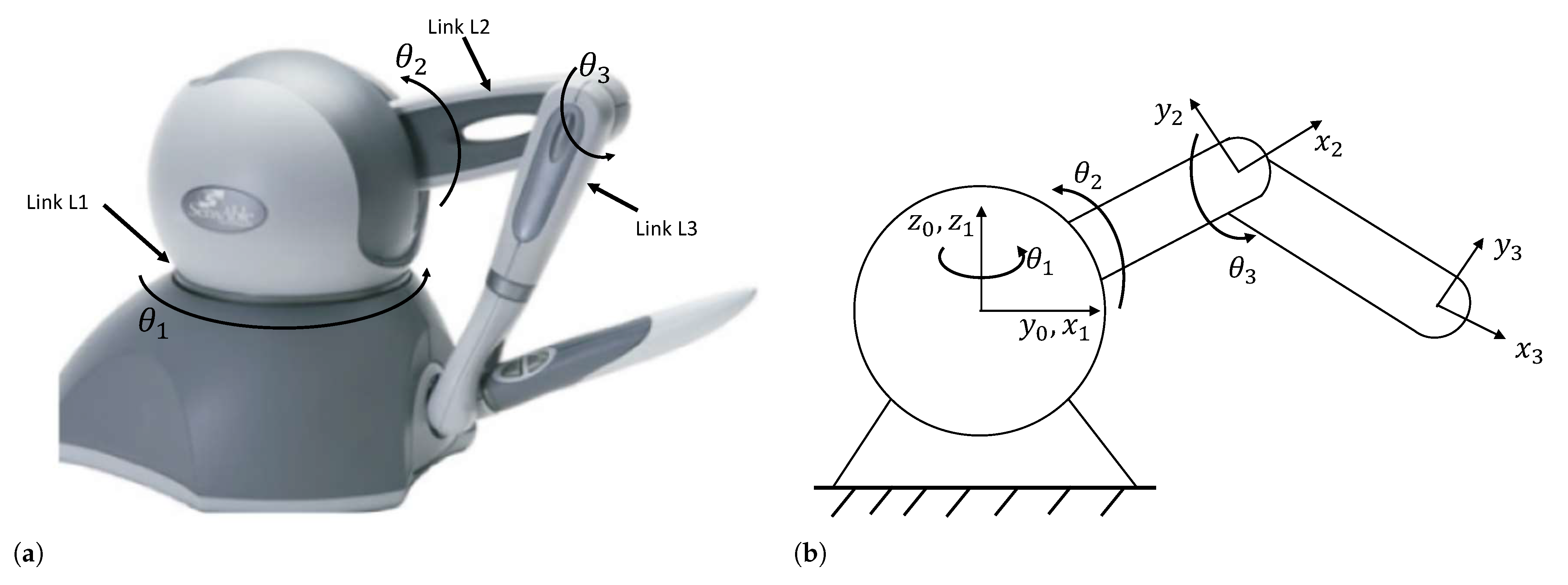
2. System Description
2.1. Dynamics Model
2.2. Kinematics Model
2.3. Control Objective
3. Preliminaries
3.1. Reinforcement Learning
3.2. Soft Actor–Critic Algorithm
3.3. Long Short-Term Memory
3.4. Generative Adversarial Imitation Learning
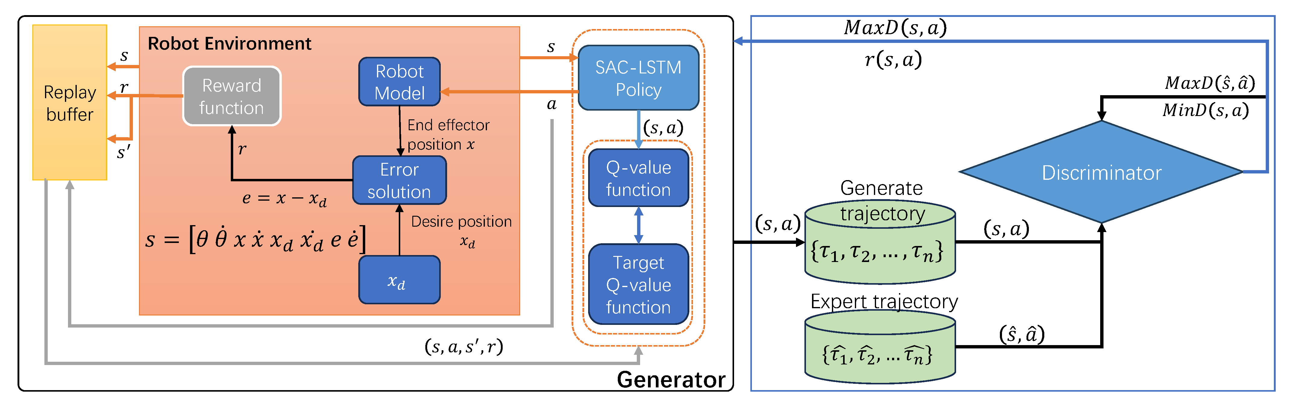
4. Control Design
4.1. Design of System Input/Output
4.2. Control Algorithm Based on SAC-LSTM
| Algorithm 1 SAC-LSTM |
Input: Policy network parameter , Q Network parameters , Input: Empty replay buffer Input: target network weights Output: Optimized parameters
|
4.3. GAIL for Robot Manipulator Trajectory Tracking
| Algorithm 2 SL-GAIL |
Input: Expert demonstration data , Policy network parameter , Discriminator network parameters Output: Optimal policy parameters
|
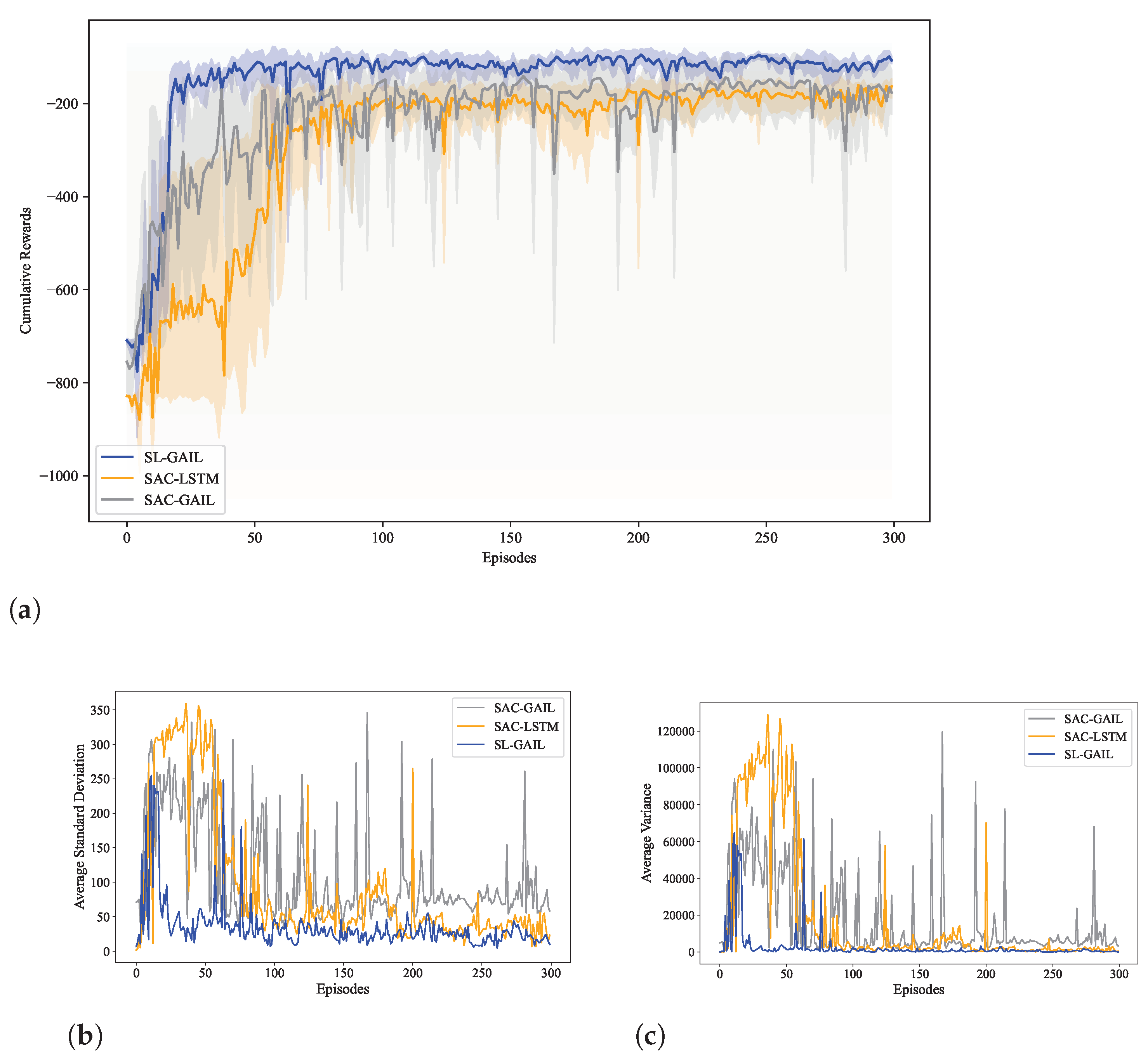
5. Simulation
5.1. Training Performance
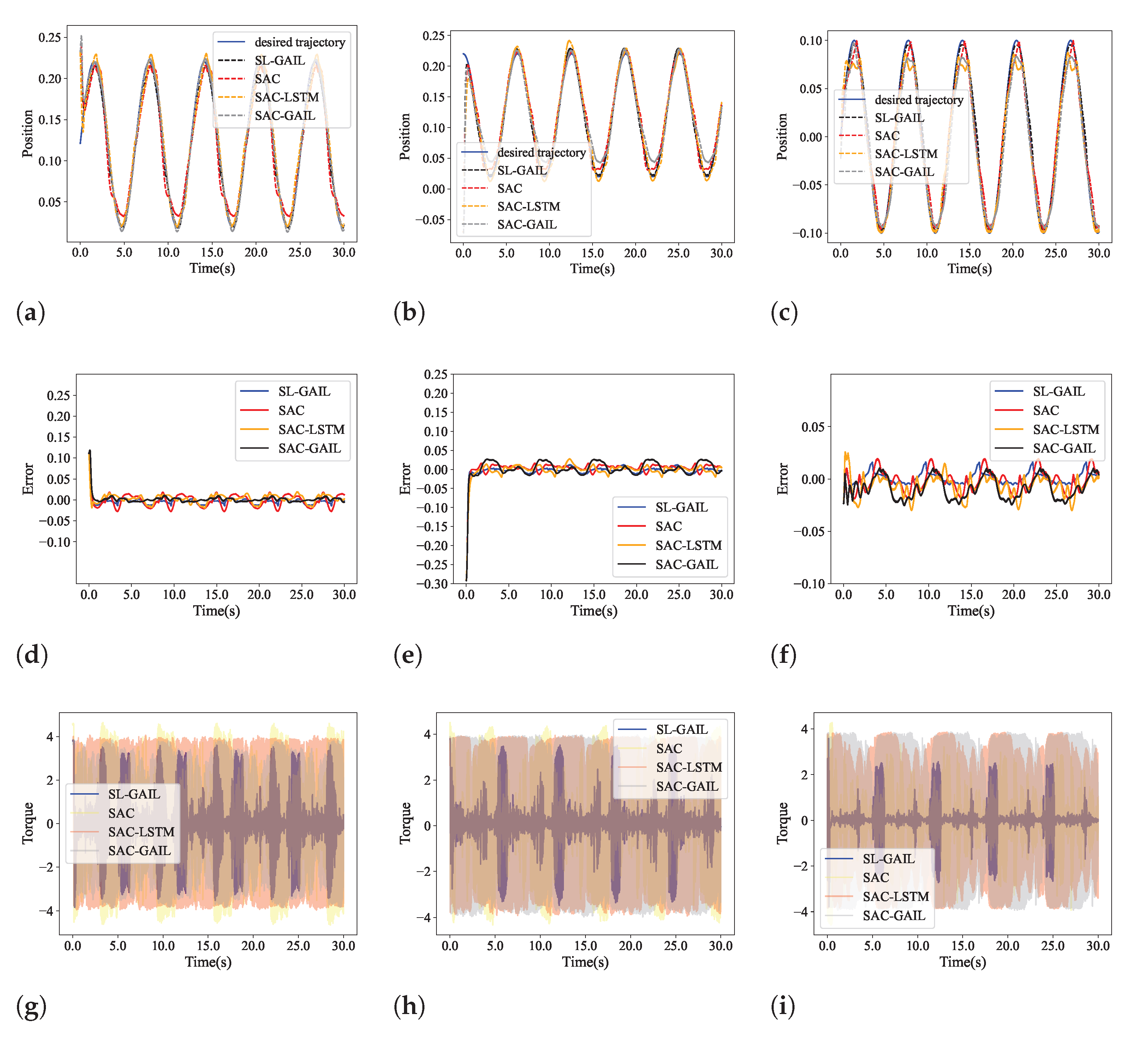
5.2. Control Performance
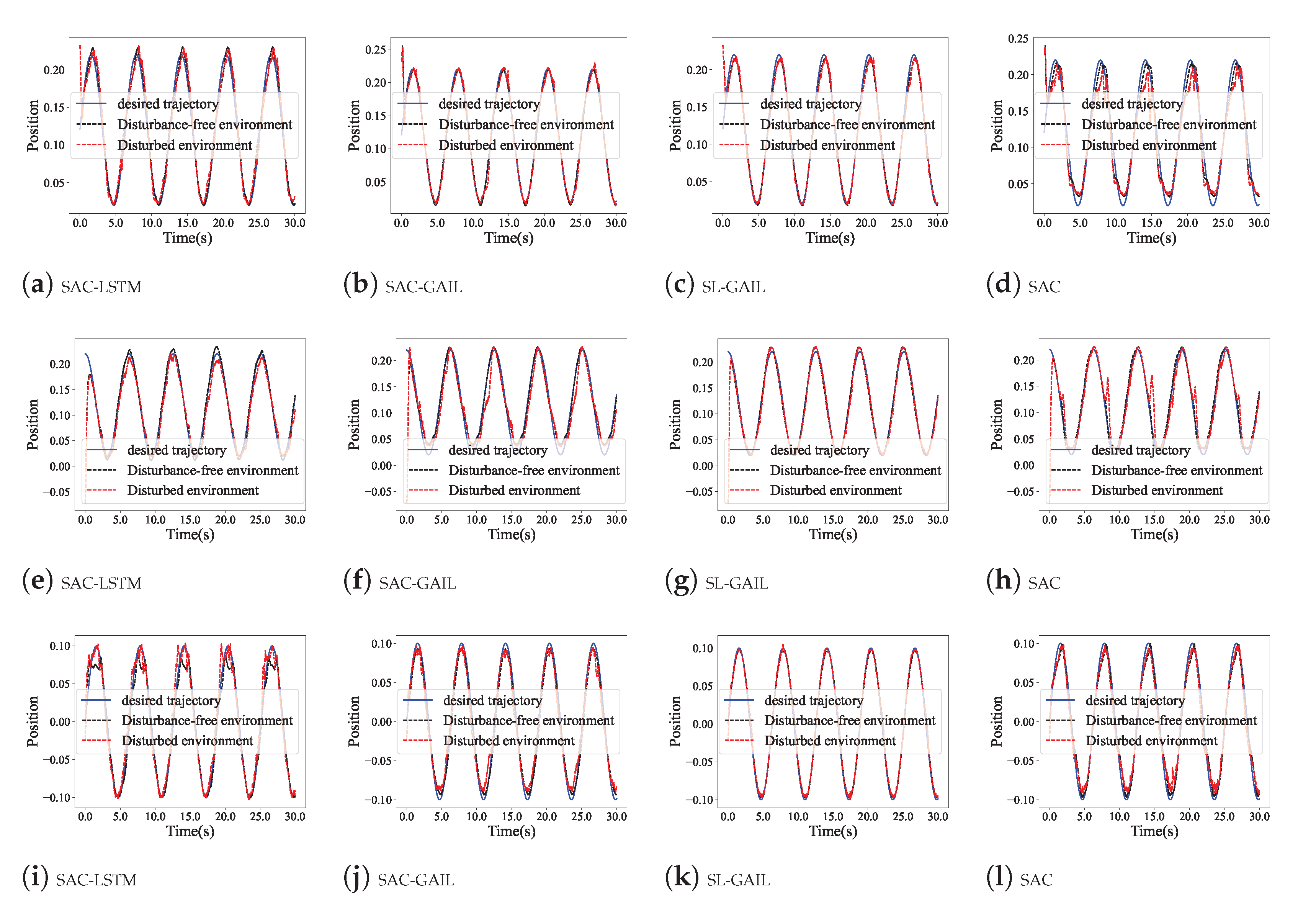
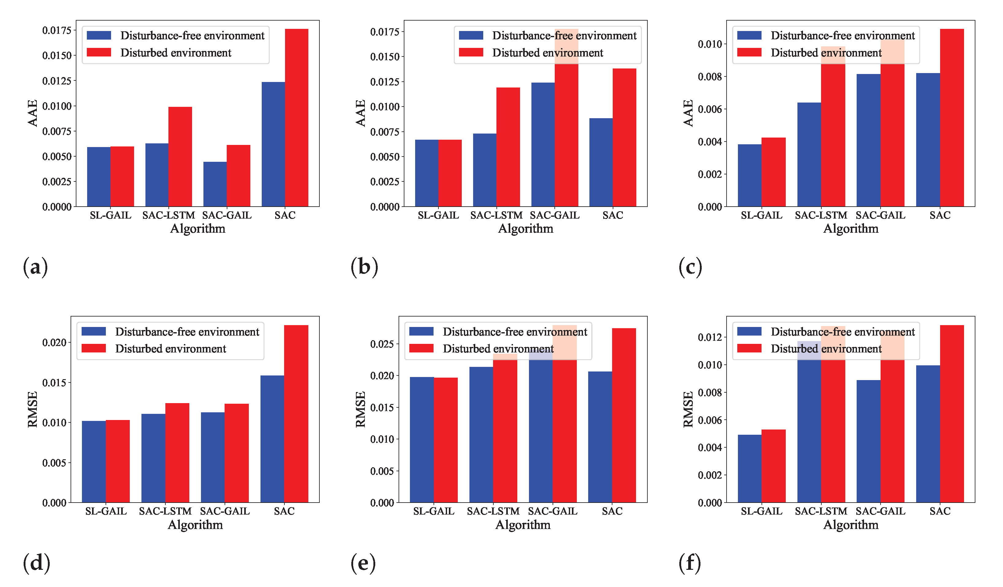
5.3. Anti-Interference Performance
6. Conclusions
Author Contributions
Funding
Institutional Review Board Statement
Data Availability Statement
Acknowledgments
Conflicts of Interest
Appendix A

| Parameter | Value | Parameter | Value |
|---|---|---|---|
| g | |||
| Parameter | Value | Parameter | Value |
|---|---|---|---|
| learning rate of actor | 0.0003 | learning rate of critic | 0.003 |
| learning rate of discriminator | 0.001 | learning rate of | 0.0003 |
| soft update parameter | 0.005 | buffer size | 1,000,000 |
| minimal size | 5000 | batch size | 256 |
| lstm hidden size | 128 | lstm num layers | 1 |
| Symbol | Description |
|---|---|
| The optimal state-value function, representing the maximum expected return at state s. | |
| The policy probability of selecting action a at state s. | |
| The transition probability from state s to state by action a. | |
| The reward for transitioning from state s to state under action a. | |
| The optimal action-value function, representing the maximum expected return for taking action a at state s. | |
| The policy entropy, representing the randomness of the policy at state . |
References
- Abdelmaksoud, S.I.; Al-Mola, M.H.; Abro, G.E.M.; Asirvadam, V.S. In-Depth Review of Advanced Control Strategies and Cutting-Edge Trends in Robot Manipulators: Analyzing the Latest Developments and Techniques. IEEE Access 2024, 12, 47672–47701. [Google Scholar] [CrossRef]
- Poór, P.; Broum, T.; Basl, J. Role of collaborative robots in industry 4.0 with target on education in industrial engineering. In Proceedings of the 2019 4th International Conference on Control, Robotics and Cybernetics (CRC), Tokyo, Japan, 27–30 September 2019; pp. 42–46. [Google Scholar]
- Hu, Y.; Wang, W.; Liu, H.; Liu, L. Reinforcement learning tracking control for robotic manipulator with kernel-based dynamic model. IEEE Trans. Neural Netw. Learn. Syst. 2020, 31, 3570–3578. [Google Scholar] [CrossRef] [PubMed]
- Chotikunnan, P.; Chotikunnan, R. Dual design pid controller for robotic manipulator application. J. Robot. Control (JRC) 2023, 4, 23–34. [Google Scholar] [CrossRef]
- Dou, W.; Ding, S.; Yu, X. Event-triggered second-order sliding-mode control of uncertain nonlinear systems. IEEE Trans. Syst. Man Cybern. Syst. 2023, 53, 7269–7279. [Google Scholar] [CrossRef]
- Pan, J. Fractional-order sliding mode control of manipulator combined with disturbance and state observer. Robot. Auton. Syst. 2025, 183, 104840. [Google Scholar] [CrossRef]
- Li, T.; Li, S.; Sun, H.; Lv, D. The fixed-time observer-based adaptive tracking control for aerial flexible-joint robot with input saturation and output constraint. Drones 2023, 7, 348. [Google Scholar] [CrossRef]
- Cho, M.; Lee, Y.; Kim, K.S. Model predictive control of autonomous vehicles with integrated barriers using occupancy grid maps. IEEE Robot. Autom. Lett. 2023, 8, 2006–2013. [Google Scholar] [CrossRef]
- Deng, W.; Zhou, H.; Zhou, J.; Yao, J. Neural network-based adaptive asymptotic prescribed performance tracking control of hydraulic manipulators. IEEE Trans. Syst. Man Cybern. Syst. 2022, 53, 285–295. [Google Scholar] [CrossRef]
- Li, S.; Nguyen, H.T.; Cheah, C.C. A theoretical framework for end-to-end learning of deep neural networks with applications to robotics. IEEE Access 2023, 11, 21992–22006. [Google Scholar] [CrossRef]
- Zhu, Z.; Lin, K.; Jain, A.K.; Zhou, J. Transfer learning in deep reinforcement learning: A survey. IEEE Trans. Pattern Anal. Mach. Intell. 2023, 45, 13344–13362. [Google Scholar] [CrossRef]
- Tran, V.P.; Mabrok, M.A.; Anavatti, S.G.; Garratt, M.A.; Petersen, I.R. Robust fuzzy q-learning-based strictly negative imaginary tracking controllers for the uncertain quadrotor systems. IEEE Trans. Cybern. 2023, 53, 5108–5120. [Google Scholar] [CrossRef] [PubMed]
- Liu, J.; Zhou, Y.; Gao, J.; Yan, W. Visual servoing gain tuning by sarsa: An application with a manipulator. In Proceedings of the 2023 3rd International Conference on Robotics and Control Engineering, Nanjing, China, 12–14 May 2023; pp. 103–107. [Google Scholar]
- Xu, H.; Fan, J.; Wang, Q. Model-based reinforcement learning for trajectory tracking of musculoskeletal robots. In Proceedings of the 2023 IEEE International Instrumentation and Measurement Technology Conference (I2MTC), Kuala Lumpur, Malaysia, 22–25 May 2023; pp. 1–6. [Google Scholar]
- Li, X.; Shang, W.; Cong, S. Offline reinforcement learning of robotic control using deep kinematics and dynamics. IEEE/ASME Trans. Mechatron. 2023, 29, 2428–2439. [Google Scholar] [CrossRef]
- Zhang, S.; Pang, Y.; Hu, G. Trajectory-tracking control of robotic system via proximal policy optimization. In Proceedings of the 2019 IEEE International Conference on Cybernetics and Intelligent Systems (CIS) and IEEE Conference on Robotics, Automation and Mechatronics (RAM), Bangkok, Thailand, 18–20 November 2019; pp. 380–385. [Google Scholar]
- Schulman, J.; Wolski, F.; Dhariwal, P.; Radford, A.; Klimov, O. Proximal policy optimization algorithms. CoRR arXiv 2017, arXiv:abs/1707.06347. [Google Scholar]
- Hu, Y.; Si, B. A reinforcement learning neural network for robotic manipulator control. Neural Comput. 2018, 30, 1983–2004. [Google Scholar] [CrossRef]
- Lei, W.; Sun, G. End-to-end active non-cooperative target tracking of free-floating space manipulators. Trans. Inst. Meas. Control 2023, 416, 379–394. [Google Scholar] [CrossRef]
- Song, D.; Gan, W.; Yao, P. Search and tracking strategy of autonomous surface underwater vehicle in oceanic eddies based on deep reinforcement learning. Appl. Soft Comput. 2023, 132, 109902. [Google Scholar] [CrossRef]
- Ho, J.; Ermon, S. Generative adversarial imitation learning. Adv. Neural Inf. Process. Syst. 2016, 29, 2016. [Google Scholar]
- Ning, G.; Liang, H.; Zhang, X.; Liao, H. Inverse-reinforcement-learning-based robotic ultrasound active compliance control in uncertain environments. IEEE Trans. Ind. Electron. 2024, 71, 1686–1696. [Google Scholar] [CrossRef]
- Goodfellow, I.; Pouget-Abadie, J.; Mirza, M.; Xu, B.; Warde-Farley, D.; Ozair, S.; Courville, A.; Bengio, Y. Generative adversarial networks. Commun. Acm 2020, 63, 139–144. [Google Scholar] [CrossRef]
- Jiang, D.; Huang, J.; Fang, Z.; Cheng, C.; Sha, Q.; He, B.; Li, G. Generative adversarial interactive imitation learning for path following of autonomous underwater vehicle. Ocean. Eng. 2022, 260, 111971. [Google Scholar] [CrossRef]
- Chaysri, P.; Spatharis, C.; Blekas, K.; Vlachos, K. Unmanned surface vehicle navigation through generative adversarial imitation learning. Ocean. Eng. 2023, 282, 114989. [Google Scholar] [CrossRef]
- Schulman, J.; Levine, S.; Abbeel, P.; Jordan, M.; Moritz, P. Trust region policy optimization. In Proceedings of the International Conference on Machine Learning, PMLR, Lille, France, 7–9 July 2015; pp. 1889–1897. [Google Scholar]
- Pecioski, D.; Gavriloski, V.; Domazetovska, S.; Ignjatovska, A. An overview of reinforcement learning techniques. In Proceedings of the 2023 12th Mediterranean Conference on Embedded Computing (MECO), Budva, Montenegro, 6–10 June 2023; IEEE: New York, NY, USA, 2023; pp. 1–4. [Google Scholar]
- Zhou, Y.; Lu, M.; Liu, X.; Che, Z.; Xu, Z.; Tang, J.; Zhang, Y.; Peng, Y.; Peng, Y. Distributional generative adversarial imitation learning with reproducing kernel generalization. Neural Netw. 2023, 165, 43–59. [Google Scholar] [CrossRef] [PubMed]
- Spong, M.W.; Hutchinson, S.; Vidyasagar, M. Robot Modeling and Control; John Wiley & Sons: Hoboken, NJ, USA, 2020. [Google Scholar]
- Wan, L.; Pan, Y.J.; Shen, H. Improving synchronization performance of multiple euler–lagrange systems using nonsingular terminal sliding mode control with fuzzy logic. IEEE/ASME Trans. Mechatron. 2021, 27, 2312–2321. [Google Scholar] [CrossRef]
- Ma, Z.; Liu, Z.; Huang, P. Fractional-order control for uncertain teleoperated cyber-physical system with actuator fault. IEEE/ASME Trans. Mechatron. 2020, 26, 2472–2482. [Google Scholar] [CrossRef]
- Forbrigger, S. Prediction-Based Haptic Interfaces to Improve Transparency for Complex Virtual Environments. 2017. Available online: https://dalspace.library.dal.ca/items/d436a139-31ec-4571-8247-4b5d70530513 (accessed on 17 December 2024).
- Liu, Y.C.; Khong, M.H. Adaptive control for nonlinear teleoperators with uncertain kinematics and dynamics. IEEE/ASME Trans. Mechatron. 2015, 20, 2550–2562. [Google Scholar] [CrossRef]
- Maheshwari, A.; Rautela, A.; Rayguru, M.M.; Valluru, S.K. Adaptive-optimal control for reconfigurable robots. In Proceedings of the 2023 International Conference on Device Intelligence, Computing and Communication Technologies, (DICCT), Dehradun, India, 17–18 March 2023; pp. 511–514. [Google Scholar]
- Li, F.; Fu, M.; Chen, W.; Zhang, F.; Zhang, H.; Qu, H.; Yi, Z. Improving exploration in actor–critic with weakly pessimistic value estimation and optimistic policy optimization. IEEE Trans. Neural Netw. Learn. Syst. 2022, 35, 8783–8796. [Google Scholar] [CrossRef]
- Hochreiter, S.; Schmidhuber, J. Long short-term memory. Neural Comput. 1997, 9, 1735–1780. [Google Scholar] [CrossRef]
- Zhang, L.; Liu, Q.; Huang, Z.; Wu, L. Learning unbiased rewards with mutual information in adversarial imitation learning. In Proceedings of the ICASSP 2023—2023 IEEE International Conference on Acoustics, Speech and Signal Processing (ICASSP), Seoul, Republic of Korea, 4–10 June 2023; pp. 1–5. [Google Scholar]
- Huang, F.; Xu, J.; Wu, D.; Cui, Y.; Yan, Z.; Xing, W.; Zhang, X. A general motion controller based on deep reinforcement learning for an autonomous underwater vehicle with unknown disturbances. Eng. Appl. Artif. Intell. 2023, 117, 105589. [Google Scholar] [CrossRef]
- Wang, T.; Wang, F.; Xie, Z.; Qin, F. Curiosity model policy optimization for robotic manipulator tracking control with input saturation in uncertain environment. Front. Neurorobot. 2024, 18, 1376215. [Google Scholar] [CrossRef]


| Category | Method | Main Constraints | References |
|---|---|---|---|
| Hydraulic Manipulators | RBFNN-based adaptive asymptotic method | Complex mathematical models, uncertain dynamics | [9] |
| Serial Manipulators | PID, sliding-mode control, adaptive control | High reliance on precise models, many control parameters | [4,5,7] |
| Free-floating Manipulators | DRL-based SAC-RNN | Unknown dynamics, high control complexity | [19] |
| 3-DoF Manipulators | SARSA algorithm | Weak capability for handling continuous state spaces | [13] |
| 2-DoF Manipulators | Actor–critic RL | Deadzone problem, nonlinear dynamic characteristics | [18] |
| Pneumatic Musculoskeletal Robots | Model-based RL (MBRL) methods | Difficulty in learning effective control policies | [14] |
| Autonomous Underwater Vehicles (AUVs) | GAIL-based policy learning | Low data efficiency, challenging generalization to unknown environments | [24] |
| Unmanned Surface Vehicles (USVs) | GAIL combined with PPO or TRPO | Low sample efficiency, insufficient exploration capability | [25] |
| Robotic Arms and Mobile Robots | Distributed PPO combined with LSTM | Insufficient handling of temporal state dependencies | [16] |
| Underactuated Autonomous Surface/Underwater Vehicles (UASUVs) | SAC combined with LSTM | Training instability, input disturbances | [20] |
| Axe Algorithms | SAC | SAC-GAIL | SAC-LSTM | SL-GAIL | |
|---|---|---|---|---|---|
| X | AAE | 0.0123 | 0.0044 | 0.0062 | 0.0058 |
| AAT | 3.5349 | 1.9642 | 2.2820 | 1.1057 | |
| RMSE | 0.0158 | 0.0112 | 0.0110 | 0.0101 | |
| Y | AAE | 0.0088 | 0.0123 | 0.0072 | 0.0066 |
| AAT | 3.4609 | 2.6186 | 1.8884 | 0.7469 | |
| RMSE | 0.0206 | 0.0240 | 0.0213 | 0.01975 | |
| Z | AAE | 0.0081 | 0.0081 | 0.0063 | 0.0038 |
| AAT | 2.9630 | 2.3313 | 0.9714 | 0.4388 | |
| RMSE | 0.0099 | 0.0088 | 0.0116 | 0.0052 | |
| Axes Algorithms | SAC | SAC-GAIL | SAC-LSTM | SL-GAIL | |
|---|---|---|---|---|---|
| X | DFENV | 0.0123 | 0.0044 | 0.0062 | 0.0058 |
| DENV | 0.0176 | 0.0061 | 0.0098 | 0.0059 | |
| Y | DFENV | 0.0088 | 0.0123 | 0.0072 | 0.0066 |
| DENV | 0.0137 | 0.0177 | 0.0118 | 0.0066 | |
| Z | DFENV | 0.0081 | 0.0081 | 0.0063 | 0.0038 |
| DENV | 0.0099 | 0.0102 | 0.0098 | 0.0042 | |
| Axes Algorithms | SAC | SAC-GAIL | SAC-LSTM | SL-GAIL | |
|---|---|---|---|---|---|
| X | DFENV | 0.0158 | 0.0112 | 0.0110 | 0.0101 |
| DENV | 0.0221 | 0.0123 | 0.0124 | 0.0102 | |
| Y | DFENV | 0.0206 | 0.0240 | 0.0213 | 0.0197 |
| DENV | 0.0274 | 0.0279 | 0.0234 | 0.0196 | |
| Z | DFENV | 0.0099 | 0.0088 | 0.0116 | 0.0049 |
| DENV | 0.0128 | 0.0124 | 0.0127 | 0.0052 | |
Disclaimer/Publisher’s Note: The statements, opinions and data contained in all publications are solely those of the individual author(s) and contributor(s) and not of MDPI and/or the editor(s). MDPI and/or the editor(s) disclaim responsibility for any injury to people or property resulting from any ideas, methods, instructions or products referred to in the content. |
© 2024 by the authors. Licensee MDPI, Basel, Switzerland. This article is an open access article distributed under the terms and conditions of the Creative Commons Attribution (CC BY) license (https://creativecommons.org/licenses/by/4.0/).
Share and Cite
Hu, J.; Wang, F.; Li, X.; Qin, Y.; Guo, F.; Jiang, M. Trajectory Tracking Control for Robotic Manipulator Based on Soft Actor–Critic and Generative Adversarial Imitation Learning. Biomimetics 2024, 9, 779. https://doi.org/10.3390/biomimetics9120779
Hu J, Wang F, Li X, Qin Y, Guo F, Jiang M. Trajectory Tracking Control for Robotic Manipulator Based on Soft Actor–Critic and Generative Adversarial Imitation Learning. Biomimetics. 2024; 9(12):779. https://doi.org/10.3390/biomimetics9120779
Chicago/Turabian StyleHu, Jintao, Fujie Wang, Xing Li, Yi Qin, Fang Guo, and Ming Jiang. 2024. "Trajectory Tracking Control for Robotic Manipulator Based on Soft Actor–Critic and Generative Adversarial Imitation Learning" Biomimetics 9, no. 12: 779. https://doi.org/10.3390/biomimetics9120779
APA StyleHu, J., Wang, F., Li, X., Qin, Y., Guo, F., & Jiang, M. (2024). Trajectory Tracking Control for Robotic Manipulator Based on Soft Actor–Critic and Generative Adversarial Imitation Learning. Biomimetics, 9(12), 779. https://doi.org/10.3390/biomimetics9120779