
A Multi-Agent Reinforcement Learning Method for Omnidirectional Walking of Bipedal Robots

Abstract
:1. Introduction
- (1)
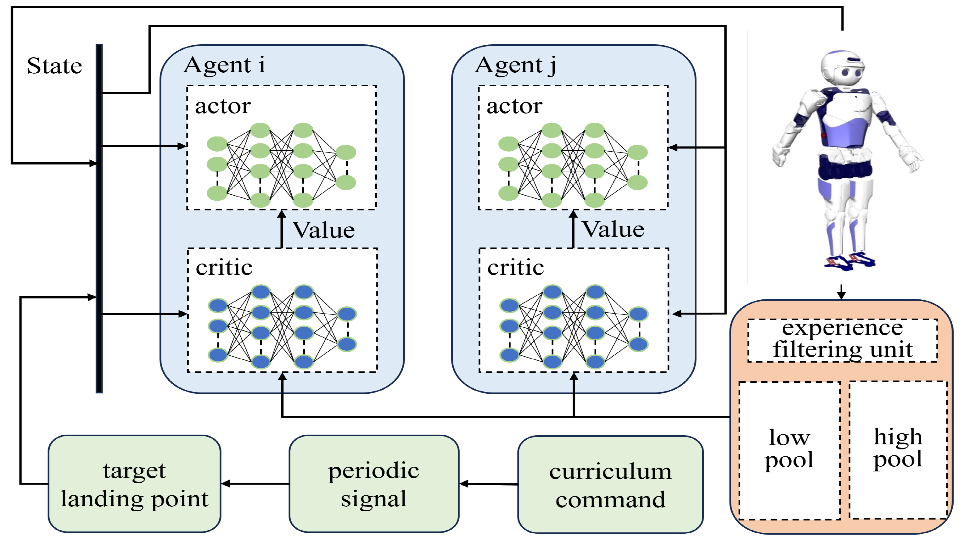
- A novel approach to multi-agent RL is constructed which is based on the actor–critic framework. A combinatorial optimization approach is employed to maximize the cumulative reward and policy entropy. Additionally, a new experience replay mechanism is designed specifically for multi-agent RL methods.
- (2)
- A new periodic gait function is designed and incorporated as an objective into our RL policy. Our periodic gait function enables bipedal gaits to exhibit symmetry and periodicity.
- (3)
- A curriculum learning method based on Gaussian distribution discretization is proposed. During the training process, the turning angle is dynamically adjusted, and a single strategy is used to achieve omnidirectional walking with different turning angles.
2. Related Work
3. Preliminaries
3.1. Actor–Critic Algorithm
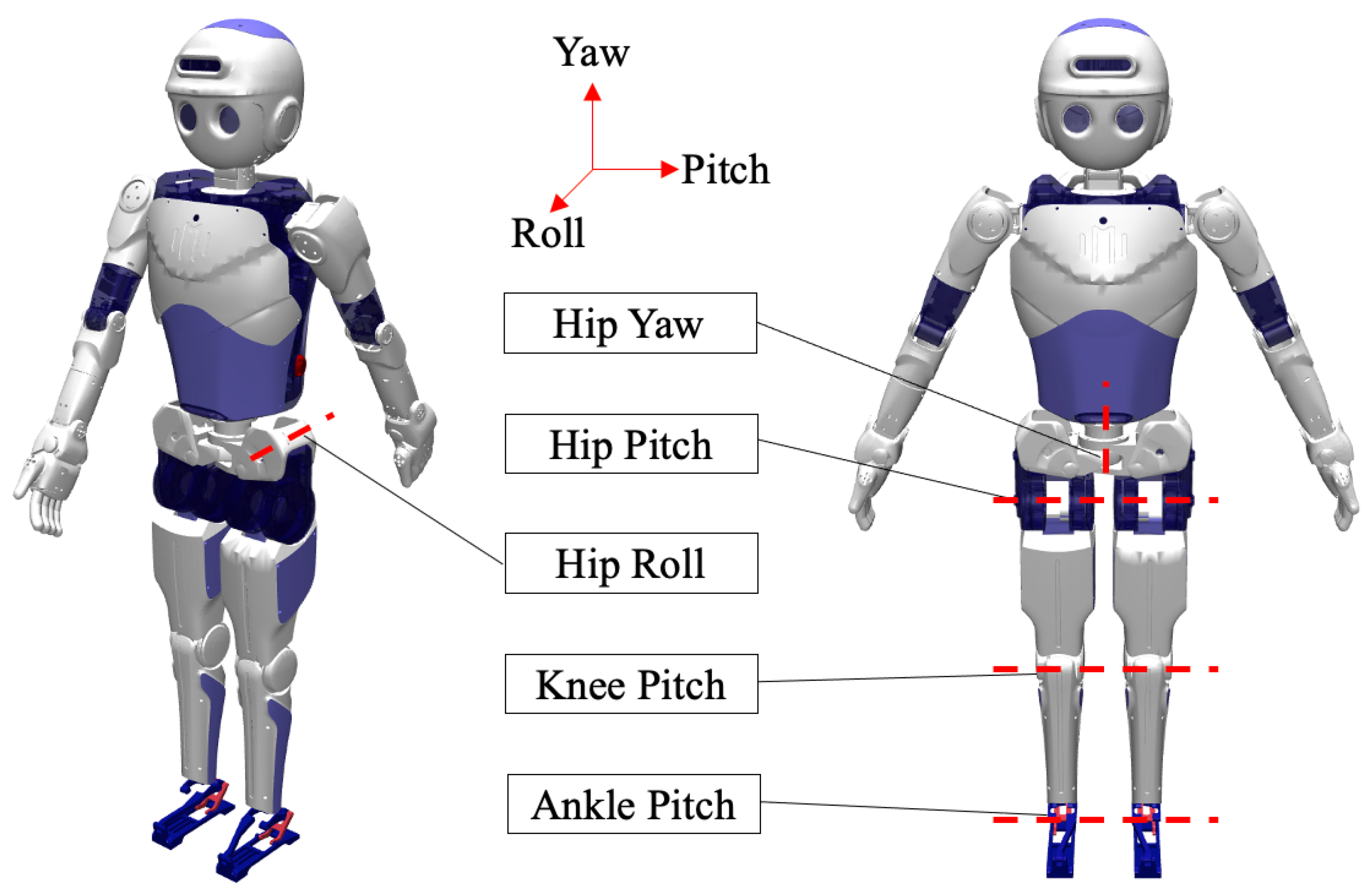
3.2. Robotics Platform
4. Method
4.1. Robot Operating System Footstep Planner
4.2. Bipedal Periodic Objective Function
4.3. Multi-Agent Systems and Policy Entropy
4.4. Heterogeneous Policy Experience Replay Mechanism Based on Euclidean Distance
4.5. Design of Curriculum Learning Framework for Omnidirectional Gait
| Algorithm 1 Curriculum learning algorithm |
|
4.6. Markov Decision Process Modeling for Omnidirectional Gait
- (1)
- Statespace
- (2)
- Action space
- (3)
- Reward Functions
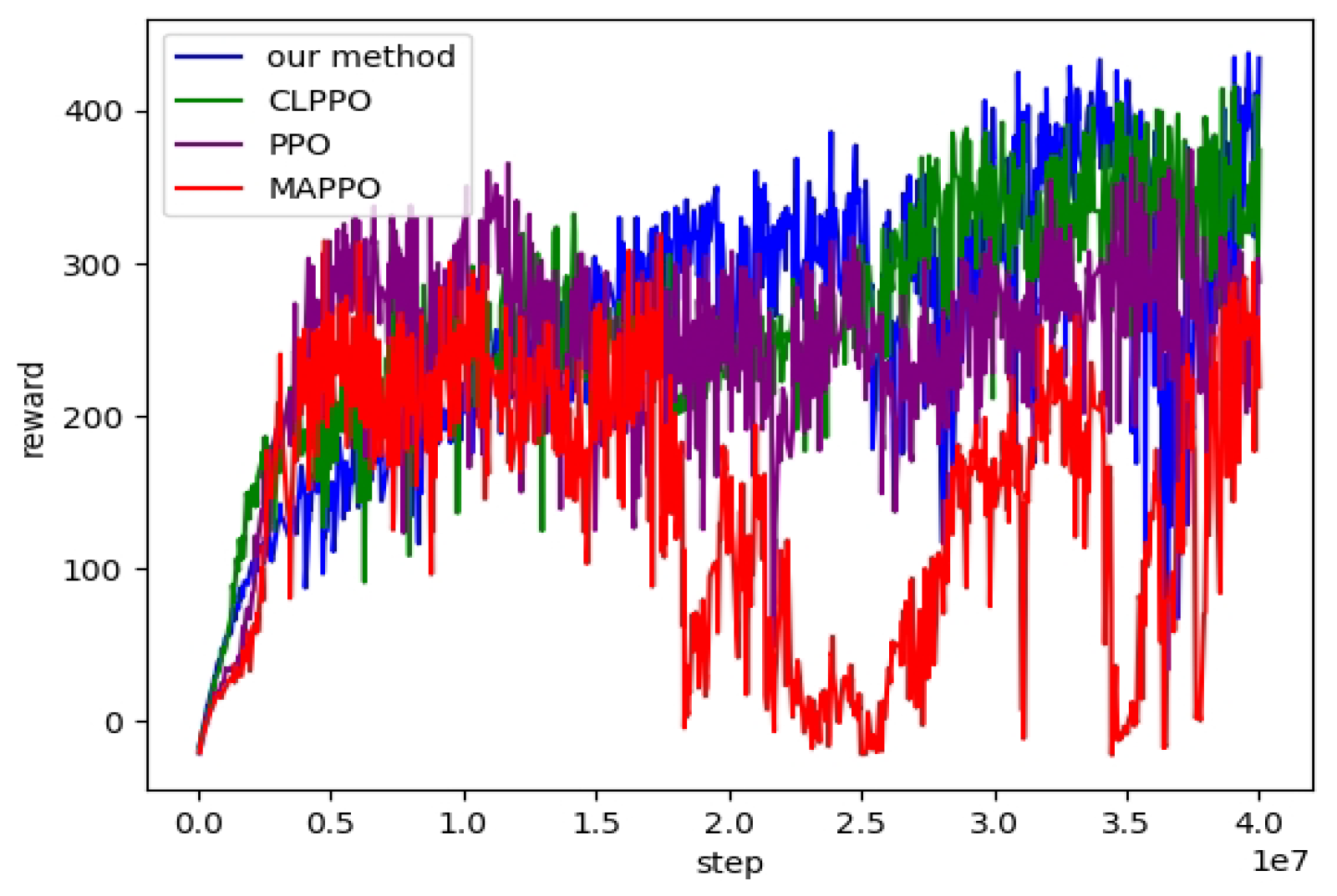
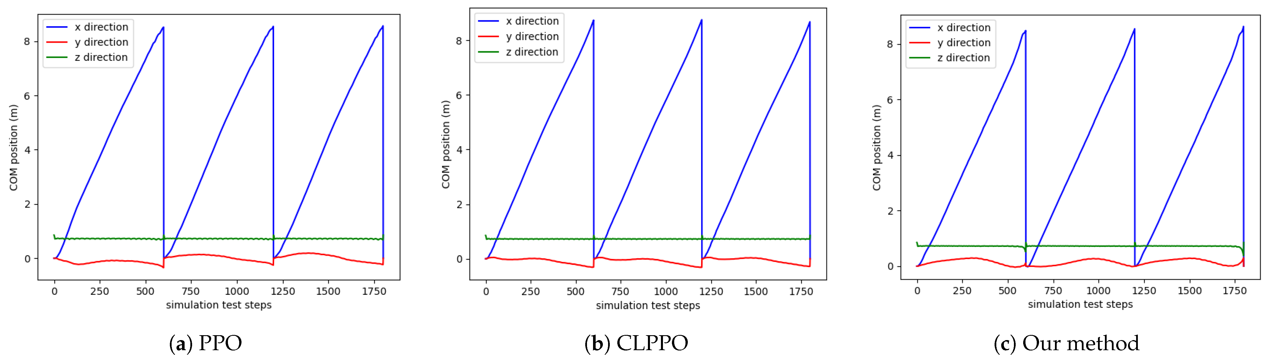
5. Results and Discussion
5.1. Experimental Environment and Settings
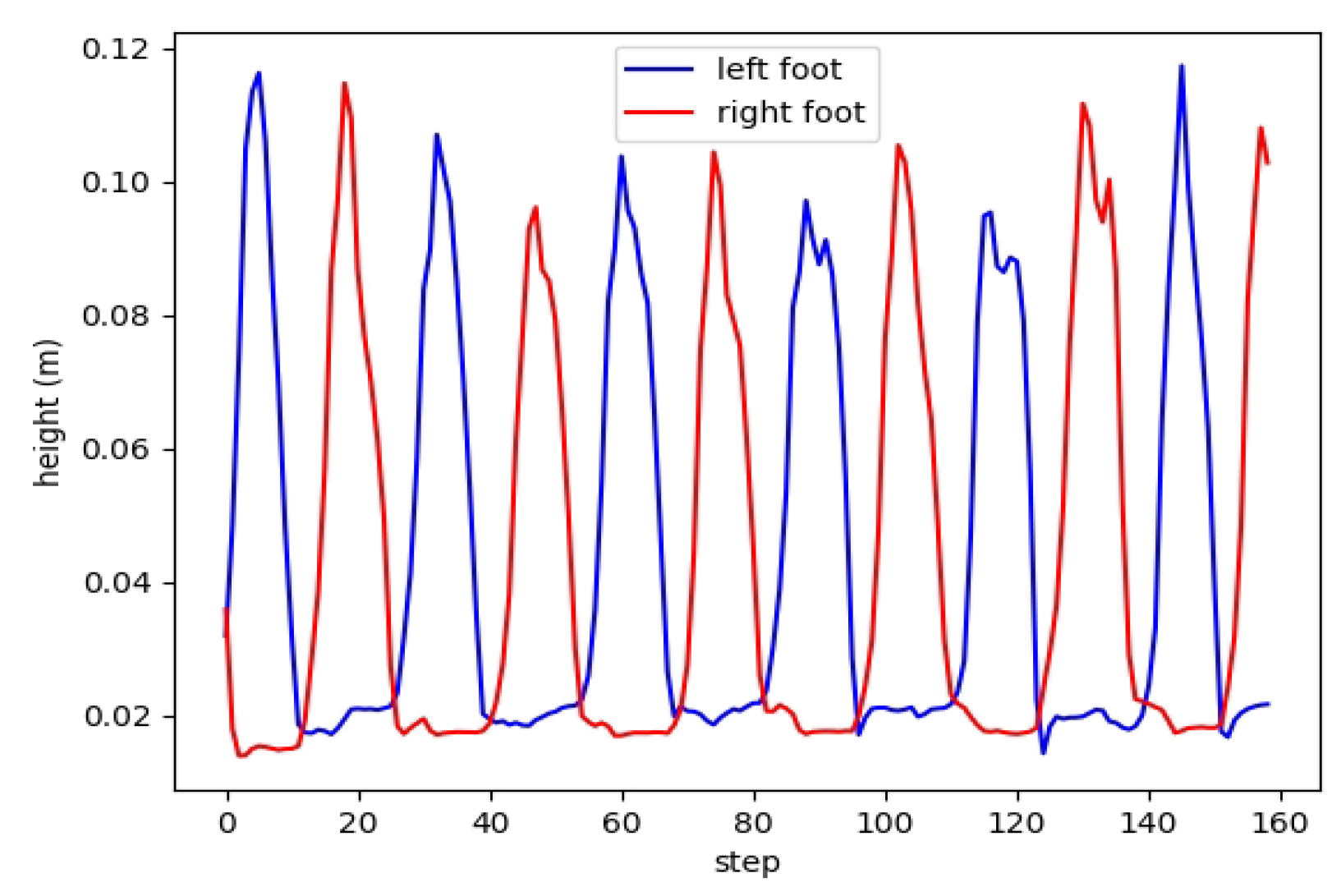
5.2. Straight Gait
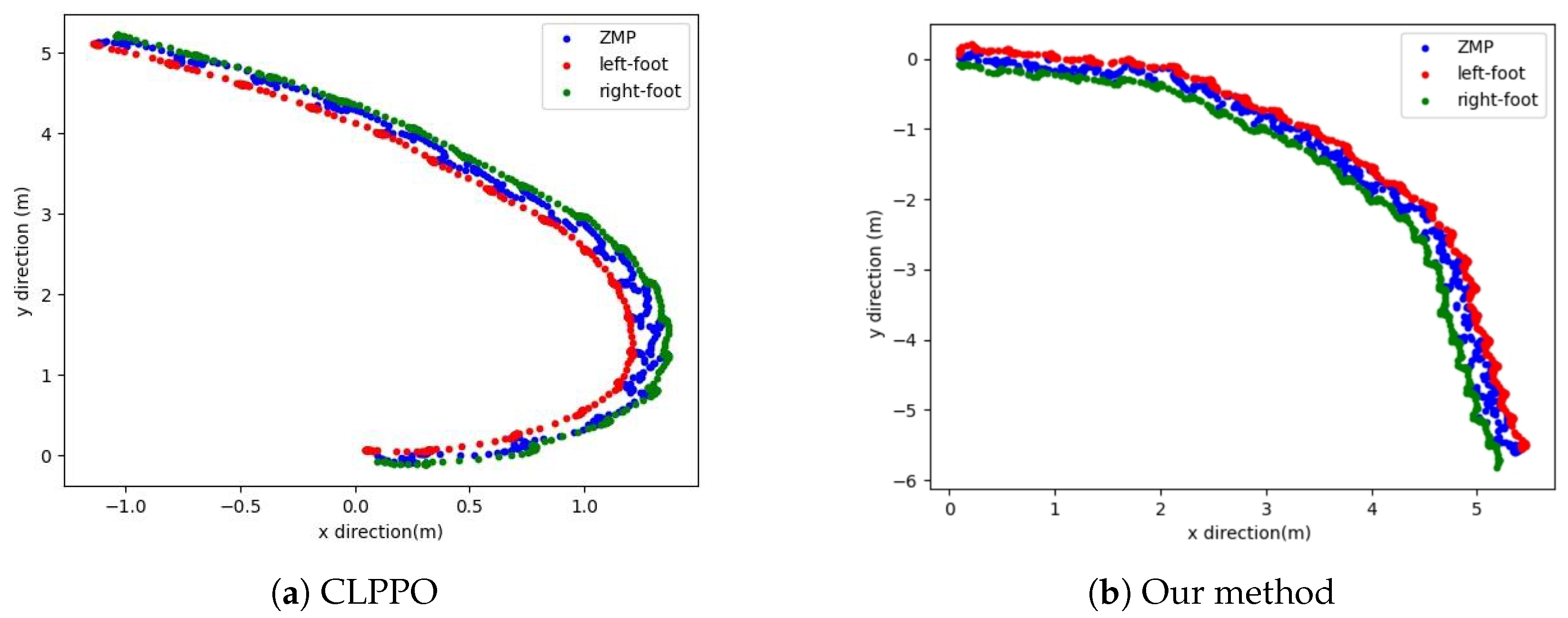
5.3. Steering Gait
6. Conclusions
Author Contributions
Funding
Institutional Review Board Statement
Data Availability Statement
Conflicts of Interest
References
- Do, H.M.; Welch, K.C.; Sheng, W. Soham: A sound-based human activity monitoring framework for home service robots. IEEE Trans. Autom. Sci. Eng. 2021, 19, 2369–2383. [Google Scholar] [CrossRef]
- Huang, J.K.; Grizzle, J.W. Efficient anytime clf reactive planning system for a bipedal robot on undulating terrain. IEEE Trans. Robot. 2023, 39, 2093–2110. [Google Scholar] [CrossRef]
- Wang, Z.; Kou, L.; Ke, W.; Chen, Y.; Bai, Y.; Li, Q.; Lu, D. A Spring Compensation Method for a Low-Cost Biped Robot Based on Whole Body Control. Biomimetics 2023, 8, 126. [Google Scholar] [CrossRef] [PubMed]
- Singh, B.; Vijayvargiya, A.; Kumar, R. Mapping model for genesis of joint trajectory using human gait dataset. In Proceedings of the 2021 Smart Technologies, Communication and Robotics (STCR), Sathyamangalam, India, 9–10 October 2021; IEEE: Piscataway, NJ, USA, 2021; pp. 1–5. [Google Scholar]
- Zhao, Y.; Gao, Y.; Sun, Q.; Tian, Y.; Mao, L.; Gao, F. A real-time low-computation cost human-following framework in outdoor environment for legged robots. Robot. Auton. Syst. 2021, 146, 103899. [Google Scholar] [CrossRef]
- Park, H.Y.; Kim, J.H.; Yamamoto, K. A new stability framework for trajectory tracking control of biped walking robots. IEEE Trans. Ind. Inform. 2022, 18, 6767–6777. [Google Scholar] [CrossRef]
- Sugihara, T.; Imanishi, K.; Yamamoto, T.; Caron, S. 3D biped locomotion control including seamless transition between walking and running via 3D ZMP manipulation. In Proceedings of the 2021 IEEE International Conference on Robotics and Automation (ICRA), Xi’an, China, 30 May–5 June 2021; IEEE: Piscataway, NJ, USA, 2021; pp. 6258–6263. [Google Scholar]
- Huang, Q.; Dong, C.; Yu, Z.; Chen, X.; Li, Q.; Chen, H.; Liu, H. Resistant compliance control for biped robot inspired by humanlike behavior. IEEE/ASME Trans. Mechatronics 2022, 27, 3463–3473. [Google Scholar] [CrossRef]
- Dong, C.; Yu, Z.; Chen, X.; Chen, H.; Huang, Y.; Huang, Q. Adaptability control towards complex ground based on fuzzy logic for humanoid robots. IEEE Trans. Fuzzy Syst. 2022, 30, 1574–1584. [Google Scholar] [CrossRef]
- Hong, Y.D.; Lee, B. Real-time feasible footstep planning for bipedal robots in three-dimensional environments using particle swarm optimization. IEEE/ASME Trans. Mechatronics 2019, 25, 429–437. [Google Scholar] [CrossRef]
- Wang, Y.; Li, J.P.; Xue, X.; Wang, B.C. Utilizing the correlation between constraints and objective function for constrained evolutionary optimization. IEEE Trans. Evol. Comput. 2019, 24, 29–43. [Google Scholar] [CrossRef]
- Yang, Y.; Shi, J.; Huang, S.; Ge, Y.; Cai, W.; Li, Q.; Chen, X.; Li, X.; Zhao, M. Balanced standing on one foot of biped robot based on three-particle model predictive control. Biomimetics 2022, 7, 244. [Google Scholar] [CrossRef]
- Dantec, E.; Naveau, M.; Fernbach, P.; Villa, N.; Saurel, G.; Stasse, O.; Taix, M.; Mansard, N. Whole-Body Model Predictive Control for Biped Locomotion on a Torque-Controlled Humanoid Robot. In Proceedings of the 2022 IEEE-RAS 21st International Conference on Humanoid Robots (Humanoids), Ginowan, Japan, 28–30 November 2022; pp. 638–644. [Google Scholar]
- Beranek, R.; Karimi, M.; Ahmadi, M. A behavior-based reinforcement learning approach to control walking bipedal robots under unknown disturbances. IEEE/ASME Trans. Mechatronics 2021, 27, 2710–2720. [Google Scholar] [CrossRef]
- Yuan, Y.; Li, Z.; Zhao, T.; Gan, D. DMP-based motion generation for a walking exoskeleton robot using reinforcement learning. IEEE Trans. Ind. Electron. 2019, 67, 3830–3839. [Google Scholar] [CrossRef]
- Chang, H.H.; Song, Y.; Doan, T.T.; Liu, L. Federated Multi-Agent Deep Reinforcement Learning (Fed-MADRL) for Dynamic Spectrum Access. IEEE Trans. Wirel. Commun. 2023, 22, 5337–5348. [Google Scholar] [CrossRef]
- Kumar, H.; Koppel, A.; Ribeiro, A. On the sample complexity of actor-critic method for reinforcement learning with function approximation. Mach. Learn. 2023, 112, 2433–2467. [Google Scholar] [CrossRef]
- Henderson, P.; Islam, R.; Bachman, P.; Pineau, J.; Precup, D.; Meger, D. Deep reinforcement learning that matters. In Proceedings of the AAAI Conference on Artificial Intelligence, New Orleans, LO, USA, 2–7 February 2018; Volume 32. [Google Scholar]
- Lu, F.; Zhou, G.; Zhang, C.; Liu, Y.; Chang, F.; Xiao, Z. Energy-efficient multi-pass cutting parameters optimisation for aviation parts in flank milling with deep reinforcement learning. Robot. Comput. Integr. Manuf. 2023, 81, 102488. [Google Scholar] [CrossRef]
- Yang, S.; Song, S.; Chu, S.; Song, R.; Cheng, J.; Li, Y.; Zhang, W. Heuristics Integrated Deep Reinforcement Learning for Online 3D Bin Packing. IEEE Trans. Autom. Sci. Eng. 2023, 1–12. [Google Scholar] [CrossRef]
- Schulman, J.; Wolski, F.; Dhariwal, P.; Radford, A.; Klimov, O. Proximal policy optimization algorithms. arXiv 2017, arXiv:1707.06347. [Google Scholar]
- Xie, Z.; Berseth, G.; Clary, P.; Hurst, J.; van de Panne, M. Feedback control for cassie with deep reinforcement learning. In Proceedings of the 2018 IEEE/RSJ International Conference on Intelligent Robots and Systems (IROS), Madrid, Spain, 1–5 October 2018; IEEE: Piscataway, NJ, USA, 2018; pp. 1241–1246. [Google Scholar]
- Kumar, A.; Li, Z.; Zeng, J.; Pathak, D.; Sreenath, K.; Malik, J. Adapting rapid motor adaptation for bipedal robots. In Proceedings of the 2022 IEEE/RSJ International Conference on Intelligent Robots and Systems (IROS), Kyoto, Japan, 23–27 October 2022; IEEE: Piscataway, NJ, USA, 2022; pp. 1161–1168. [Google Scholar]
- Cui, J.; Yuan, L.; He, L.; Xiao, W.; Ran, T.; Zhang, J. Multi-input autonomous driving based on deep reinforcement learning with double bias experience replay. IEEE Sensors J. 2023, 23, 11253–11261. [Google Scholar] [CrossRef]
- Ho, S.; Liu, M.; Du, L.; Gao, L.; Xiang, Y. Prototype-Guided Memory Replay for Continual Learning. IEEE Trans. Neural Netw. Learn. Syst. 2023, 1–11. [Google Scholar] [CrossRef]
- Yang, Y.; Caluwaerts, K.; Iscen, A.; Zhang, T.; Tan, J.; Sindhwani, V. Data Efficient Reinforcement Learning for Legged Robots. In Proceedings of the Conference on Robot Learning, PMLR, Cambridge, MA, USA, 30 October–1 November 2020; Volume 100, pp. 1–10. [Google Scholar]
- Hwang, K.S.; Lin, J.L.; Yeh, K.H. Learning to adjust and refine gait patterns for a biped robot. IEEE Trans. Syst. Man Cybern. Syst. 2015, 45, 1481–1490. [Google Scholar] [CrossRef]
- Qi, H.; Chen, X.; Yu, Z.; Huang, G.; Liu, Y.; Meng, L.; Huang, Q. Vertical Jump of a Humanoid Robot with CoP-Guided Angular Momentum Control and Impact Absorption. IEEE Trans. Robot. 2023, 39, 3154–3166. [Google Scholar] [CrossRef]
- Xie, Z.; Clary, P.; Dao, J.; Morais, P.; Hurst, J.; Panne, M. Learning locomotion skills for cassie: Iterative design and sim-to-real. In Proceedings of the Conference on Robot Learning, PMLR, Cambridge, MA, USA, 16–18 November 2020; pp. 317–329. [Google Scholar]
- Wu, Q.; Zhang, C.; Liu, Y. Custom Sine Waves Are Enough for Imitation Learning of Bipedal Gaits with Different Styles. In Proceedings of the 2022 IEEE International Conference on Mechatronics and Automation (ICMA), Guilin, China, 7–10 August 2022; IEEE: Piscataway, NJ, USA, 2022; pp. 499–505. [Google Scholar]
- Siekmann, J.; Godse, Y.; Fern, A.; Hurst, J. Sim-to-real learning of all common bipedal gaits via periodic reward composition. In Proceedings of the 2021 IEEE International Conference on Robotics and Automation (ICRA), Xi’an, China, 30 May–5 June 2021; IEEE: Piscataway, NJ, USA, 2021; pp. 7309–7315. [Google Scholar]
- Li, Z.; Cheng, X.; Peng, X.B.; Abbeel, P.; Levine, S.; Berseth, G.; Sreenath, K. Reinforcement learning for robust parameterized locomotion control of bipedal robots. In Proceedings of the 2021 IEEE International Conference on Robotics and Automation (ICRA), Xi’an, China, 30 May–5 June 2021; IEEE: Piscataway, NJ, USA, 2021; pp. 2811–2817. [Google Scholar]
- Duan, H.; Malik, A.; Dao, J.; Saxena, A.; Green, K.; Siekmann, J.; Fern, A.; Hurst, J. Sim-to-real learning of footstep-constrained bipedal dynamic walking. In Proceedings of the 2022 International Conference on Robotics and Automation (ICRA), Philadelphia, PA, USA, 23–27 May 2022; IEEE: Piscataway, NJ, USA, 2022; pp. 10428–10434. [Google Scholar]
- Yu, F.; Batke, R.; Dao, J.; Hurst, J.; Green, K.; Fern, A. Dynamic Bipedal Maneuvers through Sim-to-Real Reinforcement Learning. arXiv 2022, arXiv:2207.07835. [Google Scholar]
- Singh, R.P.; Benallegue, M.; Morisawa, M.; Cisneros, R.; Kanehiro, F. Learning Bipedal Walking On Planned Footsteps For Humanoid Robots. In Proceedings of the 2022 IEEE-RAS 21st International Conference on Humanoid Robots (Humanoids), Ginowan, Japan, 28–30 November 2022; IEEE: Piscataway, NJ, USA, 2022; pp. 686–693. [Google Scholar]
- Rodriguez, D.; Behnke, S. DeepWalk: Omnidirectional bipedal gait by deep reinforcement learning. In Proceedings of the 2021 IEEE International Conference on Robotics and Automation (ICRA), Xi’an, China, 30 May–5 June 2021; IEEE: Piscataway, NJ, USA, 2021; pp. 3033–3039. [Google Scholar]
- Peng, X.B.; Ma, Z.; Abbeel, P.; Levine, S.; Kanazawa, A. Amp: Adversarial motion priors for stylized physics-based character control. ACM Trans. Graph. (TOG) 2021, 40, 144. [Google Scholar] [CrossRef]
- Li, C.; Li, M.; Tao, C. A parallel heterogeneous policy deep reinforcement learning algorithm for bipedal walking motion design. Front. Neurorobotics 2023, 17, 1205775. [Google Scholar] [CrossRef]


| Joint Name | Range of Motion | Peak Torque | Joint Velocity | Stiffness | Damping |
|---|---|---|---|---|---|
| Hip Yaw | −90–90 | 133 Nm | 240/s | 0.1 | 1000 |
| Hip Pitch | −60–90 | 45.9 Nm | 576/s | 0.1 | 1000 |
| Hip Roll | −10–10 | 5000 Nm | 120/s | 0.1 | 1500 |
| Knee Pitch | −140–0 | 48.6 Nm | 540/s | 1 | 1500 |
| Ankle Pitch | −80–80 | 28.8 Nm | 918/s | 0.01 | 100 |
| Effect | Expression |
|---|---|
| command tracking | |
| keep balance | |
| smooth action | |
| Sport termination | |
| Periodic Gait | |
| Omnidirectional gait | |
Disclaimer/Publisher’s Note: The statements, opinions and data contained in all publications are solely those of the individual author(s) and contributor(s) and not of MDPI and/or the editor(s). MDPI and/or the editor(s) disclaim responsibility for any injury to people or property resulting from any ideas, methods, instructions or products referred to in the content. |
© 2023 by the authors. Licensee MDPI, Basel, Switzerland. This article is an open access article distributed under the terms and conditions of the Creative Commons Attribution (CC BY) license (https://creativecommons.org/licenses/by/4.0/).
Share and Cite
Mou, H.; Xue, J.; Liu, J.; Feng, Z.; Li, Q.; Zhang, J. A Multi-Agent Reinforcement Learning Method for Omnidirectional Walking of Bipedal Robots. Biomimetics 2023, 8, 616. https://doi.org/10.3390/biomimetics8080616
Mou H, Xue J, Liu J, Feng Z, Li Q, Zhang J. A Multi-Agent Reinforcement Learning Method for Omnidirectional Walking of Bipedal Robots. Biomimetics. 2023; 8(8):616. https://doi.org/10.3390/biomimetics8080616
Chicago/Turabian StyleMou, Haiming, Jie Xue, Jian Liu, Zhen Feng, Qingdu Li, and Jianwei Zhang. 2023. "A Multi-Agent Reinforcement Learning Method for Omnidirectional Walking of Bipedal Robots" Biomimetics 8, no. 8: 616. https://doi.org/10.3390/biomimetics8080616
APA StyleMou, H., Xue, J., Liu, J., Feng, Z., Li, Q., & Zhang, J. (2023). A Multi-Agent Reinforcement Learning Method for Omnidirectional Walking of Bipedal Robots. Biomimetics, 8(8), 616. https://doi.org/10.3390/biomimetics8080616