

An Innovative Differentiated Creative Search Based on Collaborative Development and Population Evaluation


Abstract
1. Introduction
- (1)
- Proposing a DCS variant, MSDCS, that combines three improved techniques.
- (2)
- Comprehensively examining the performance of MSDCS using the CEC2018 test suite and confirming its superiority through the Friedman test and the Wilcoxon value sum test.
- (3)
- Applying MSDCS successfully to the wireless sensor network coverage problem and engineering constrained optimization problems, showing its adaptability in facing real-world problems.
2. Differentiated Creative Search
2.1. Initialization
2.2. Differentiated Knowledge Acquisition
2.3. Creative Realism
2.4. Retrospective Assessment
3. Proposed Multi-Strategy Differentiated Creative Search
3.1. Population Evaluation Strategy (PES)
3.2. Linear Population Size Reduction Strategy (LPSR)
3.3. Collaborative Development Mechanism (CDM)
3.4. The Framework of MSDCS
| Algorithm 1. Multi Strategy Differentiated Creative Search (MSDCS) |
| 1: Initialization: Xi(i = 1, 2, 3, …, NP), FEs = 0, FEsmax |
| 2: Evaluate the fitness values of the initial population X |
| 3: while (FEs < FEsmax) do |
| 4: Calculate of each individual using Equation (12)//PES |
| 5: Sort the population in ascending order of |
| 6: for every individual, do |
| 7: Calculate the and using Equations (2) and (3) |
| 8: Randomly select using Equation (5) |
| 9: if i == N |
| 10: Update the using Equation (9) |
| 11: else if |
| 12: Update the using Equation (8) |
| 13: else |
| 14: Update the using Equation (6) |
| 15: end if |
| 16: Update the Xnewi using Equation (4) |
| 17: FEs = Fes + 1 |
| 18: end for |
| 19: Calculate and using Equations (14) and (15)//CDM |
| 20: Generate new individuals using Equation (16)//CDM |
| 21: FEs = Fes + Nc |
| 22: Calculate the Nnew using Equation (13)//LPSR |
| 23: Shrinking X by discarding the worst solutions |
| 24: end while |
| 25: Return best individual |
3.5. Complexity Analysis of MSDCS
4. Numerical Experiments Using CEC 2017 Test Suite
4.1. Experiment Setting and Performance Metrics
4.2. Parameter Sensitivity Analysis
4.3. Ablation Experiment
4.4. Comparison with Other Advanced Algorithms
5. Numerical Experiments Using Engineering Optimization Problem
5.1. Wireless Sensor Network Coverage Problem
5.2. Constrained Engineering Optimization
6. Conclusions
Author Contributions
Funding
Data Availability Statement
Acknowledgments
Conflicts of Interest
Appendix A

| Function | Index | DCS | DCS-PES | DCS-LPSR | DCS-CDM | MSDCS | Function | Index | DCS | DCS-PES | DCS-LPSR | DCS-CDM | MSDCS |
|---|---|---|---|---|---|---|---|---|---|---|---|---|---|
| F1 | Best | 5.749E+09 | 1.002E+02 | 1.730E+06 | 1.589E+02 | 1.000E+02 | F16 | Best | 1.812E+03 | 1.731E+03 | 1.739E+03 | 1.706E+03 | 1.708E+03 |
| Mean | 1.416E+10 | 1.006E+02 | 6.761E+06 | 1.959E+03 | 1.000E+02 | Mean | 2.139E+03 | 1.741E+03 | 1.750E+03 | 1.722E+03 | 1.727E+03 | ||
| Std | 4.455E+09 | 3.216E-01 | 3.158E+06 | 2.124E+03 | 1.786E-04 | Std | 1.598E+02 | 6.389E+00 | 7.504E+00 | 9.146E+00 | 8.155E+00 | ||
| F2 | Best | 2.182E+04 | 3.000E+02 | 1.777E+03 | 3.000E+02 | 3.000E+02 | F17 | Best | 2.449E+06 | 1.802E+03 | 6.754E+03 | 1.803E+03 | 1.800E+03 |
| Mean | 4.706E+04 | 3.000E+02 | 8.772E+03 | 3.003E+02 | 3.000E+02 | Mean | 2.549E+08 | 1.810E+03 | 1.515E+04 | 1.824E+03 | 1.805E+03 | ||
| Std | 1.740E+04 | 9.349E-06 | 3.893E+03 | 3.293E-01 | 2.735E-09 | Std | 2.261E+08 | 6.262E+00 | 6.760E+03 | 9.643E+00 | 7.111E+00 | ||
| F3 | Best | 7.774E+02 | 4.002E+02 | 4.054E+02 | 4.005E+02 | 4.001E+02 | F18 | Best | 2.783E+03 | 1.901E+03 | 1.942E+03 | 1.901E+03 | 1.900E+03 |
| Mean | 1.774E+03 | 4.011E+02 | 4.120E+02 | 4.024E+02 | 4.007E+02 | Mean | 8.309E+06 | 1.903E+03 | 2.355E+03 | 1.903E+03 | 1.901E+03 | ||
| Std | 6.895E+02 | 5.480E-01 | 5.797E+00 | 7.140E-01 | 4.802E-01 | Std | 8.178E+06 | 6.232E-01 | 5.995E+02 | 1.133E+00 | 5.817E-01 | ||
| F4 | Best | 5.899E+02 | 5.098E+02 | 5.109E+02 | 5.115E+02 | 5.103E+02 | F19 | Best | 2.263E+03 | 2.015E+03 | 2.021E+03 | 2.005E+03 | 2.008E+03 |
| Mean | 6.366E+02 | 5.207E+02 | 5.234E+02 | 5.170E+02 | 5.162E+02 | Mean | 2.375E+03 | 2.034E+03 | 2.038E+03 | 2.014E+03 | 2.020E+03 | ||
| Std | 2.293E+01 | 5.161E+00 | 4.691E+00 | 3.418E+00 | 3.861E+00 | Std | 5.961E+01 | 8.083E+00 | 6.878E+00 | 6.658E+00 | 6.720E+00 | ||
| F5 | Best | 6.465E+02 | 6.000E+02 | 6.004E+02 | 6.000E+02 | 6.000E+02 | F20 | Best | 2.278E+03 | 2.200E+03 | 2.204E+03 | 2.200E+03 | 2.200E+03 |
| Mean | 6.786E+02 | 6.000E+02 | 6.009E+02 | 6.000E+02 | 6.000E+02 | Mean | 2.406E+03 | 2.271E+03 | 2.230E+03 | 2.256E+03 | 2.264E+03 | ||
| Std | 1.370E+01 | 1.867E-03 | 2.781E-01 | 2.636E-03 | 3.299E-05 | Std | 4.711E+01 | 6.302E+01 | 4.716E+01 | 6.132E+01 | 6.064E+01 | ||
| F6 | Best | 8.880E+02 | 7.262E+02 | 7.335E+02 | 7.228E+02 | 7.203E+02 | F21 | Best | 2.557E+03 | 2.200E+03 | 2.267E+03 | 2.200E+03 | 2.300E+03 |
| Mean | 9.093E+02 | 7.329E+02 | 7.499E+02 | 7.326E+02 | 7.281E+02 | Mean | 3.554E+03 | 2.297E+03 | 2.304E+03 | 2.296E+03 | 2.300E+03 | ||
| Std | 1.523E+01 | 4.019E+00 | 6.364E+00 | 5.188E+00 | 4.288E+00 | Std | 3.922E+02 | 1.843E+01 | 1.082E+01 | 2.376E+01 | 5.324E-01 | ||
| F7 | Best | 8.570E+02 | 8.075E+02 | 8.144E+02 | 8.093E+02 | 8.079E+02 | F22 | Best | 2.736E+03 | 2.610E+03 | 2.617E+03 | 2.602E+03 | 2.604E+03 |
| Mean | 9.033E+02 | 8.210E+02 | 8.264E+02 | 8.169E+02 | 8.165E+02 | Mean | 2.796E+03 | 2.619E+03 | 2.625E+03 | 2.614E+03 | 2.613E+03 | ||
| Std | 1.358E+01 | 4.894E+00 | 5.167E+00 | 3.665E+00 | 4.026E+00 | Std | 2.490E+01 | 4.661E+00 | 3.787E+00 | 4.373E+00 | 4.436E+00 | ||
| F8 | Best | 2.591E+03 | 9.000E+02 | 9.036E+02 | 9.000E+02 | 9.000E+02 | F23 | Best | 2.846E+03 | 2.500E+03 | 2.515E+03 | 2.500E+03 | 2.500E+03 |
| Mean | 3.425E+03 | 9.000E+02 | 9.109E+02 | 9.000E+02 | 9.000E+02 | Mean | 2.932E+03 | 2.739E+03 | 2.571E+03 | 2.702E+03 | 2.722E+03 | ||
| Std | 4.504E+02 | 6.786E-07 | 4.790E+00 | 8.294E-02 | 2.978E-12 | Std | 4.990E+01 | 4.545E+01 | 6.942E+01 | 9.186E+01 | 6.047E+01 | ||
| F9 | Best | 2.458E+03 | 1.499E+03 | 1.709E+03 | 1.230E+03 | 1.437E+03 | F24 | Best | 2.986E+03 | 2.898E+03 | 2.906E+03 | 2.898E+03 | 2.898E+03 |
| Mean | 3.058E+03 | 2.068E+03 | 2.049E+03 | 1.742E+03 | 1.882E+03 | Mean | 3.810E+03 | 2.924E+03 | 2.923E+03 | 2.926E+03 | 2.927E+03 | ||
| Std | 3.212E+02 | 1.870E+02 | 1.626E+02 | 2.008E+02 | 1.643E+02 | Std | 4.016E+02 | 2.295E+01 | 1.407E+01 | 2.328E+01 | 2.232E+01 | ||
| F10 | Best | 1.465E+03 | 1.104E+03 | 1.137E+03 | 1.102E+03 | 1.103E+03 | F25 | Best | 3.845E+03 | 2.900E+03 | 2.783E+03 | 2.900E+03 | 2.900E+03 |
| Mean | 7.862E+03 | 1.106E+03 | 1.164E+03 | 1.105E+03 | 1.104E+03 | Mean | 4.601E+03 | 2.900E+03 | 2.931E+03 | 2.902E+03 | 2.900E+03 | ||
| Std | 5.270E+03 | 1.243E+00 | 1.740E+01 | 1.684E+00 | 8.064E-01 | Std | 3.360E+02 | 4.062E-04 | 3.732E+01 | 8.608E+00 | 2.980E-07 | ||
| F11 | Best | 1.464E+08 | 1.230E+03 | 3.190E+05 | 2.978E+03 | 1.200E+03 | F26 | Best | 3.168E+03 | 3.090E+03 | 3.093E+03 | 3.089E+03 | 3.090E+03 |
| Mean | 1.071E+09 | 1.386E+03 | 3.553E+06 | 1.137E+04 | 1.395E+03 | Mean | 3.319E+03 | 3.093E+03 | 3.098E+03 | 3.092E+03 | 3.094E+03 | ||
| Std | 6.320E+08 | 1.089E+02 | 2.030E+06 | 9.209E+03 | 1.311E+02 | Std | 7.996E+01 | 1.946E+00 | 2.439E+00 | 2.490E+00 | 1.543E+00 | ||
| F12 | Best | 2.253E+05 | 1.303E+03 | 1.973E+03 | 1.303E+03 | 1.301E+03 | F27 | Best | 3.464E+03 | 3.100E+03 | 3.090E+03 | 2.800E+03 | 3.100E+03 |
| Mean | 8.389E+07 | 1.310E+03 | 9.609E+03 | 1.317E+03 | 1.309E+03 | Mean | 3.851E+03 | 3.197E+03 | 3.209E+03 | 3.159E+03 | 3.168E+03 | ||
| Std | 8.428E+07 | 3.546E+00 | 6.426E+03 | 7.651E+00 | 4.157E+00 | Std | 1.342E+02 | 1.403E+02 | 8.947E+01 | 1.437E+02 | 1.257E+02 | ||
| F13 | Best | 1.654E+03 | 1.409E+03 | 1.441E+03 | 1.402E+03 | 1.401E+03 | F28 | Best | 3.419E+03 | 3.163E+03 | 3.188E+03 | 3.166E+03 | 3.153E+03 |
| Mean | 2.840E+05 | 1.416E+03 | 1.596E+03 | 1.416E+03 | 1.410E+03 | Mean | 3.744E+03 | 3.191E+03 | 3.227E+03 | 3.186E+03 | 3.180E+03 | ||
| Std | 6.030E+05 | 4.346E+00 | 2.724E+02 | 9.981E+00 | 6.457E+00 | Std | 1.483E+02 | 1.607E+01 | 2.012E+01 | 1.631E+01 | 1.488E+01 | ||
| F14 | Best | 1.531E+04 | 1.501E+03 | 1.565E+03 | 1.501E+03 | 1.501E+03 | F29 | Best | 3.125E+06 | 3.411E+03 | 3.646E+04 | 3.586E+03 | 3.415E+03 |
| Mean | 2.000E+06 | 1.503E+03 | 2.013E+03 | 1.504E+03 | 1.502E+03 | Mean | 7.109E+07 | 4.526E+04 | 4.062E+05 | 1.322E+05 | 1.140E+05 | ||
| Std | 4.195E+06 | 8.736E-01 | 4.724E+02 | 1.351E+00 | 7.093E-01 | Std | 4.385E+07 | 2.286E+05 | 4.074E+05 | 3.358E+05 | 3.433E+05 | ||
| F15 | Best | 1.926E+03 | 1.604E+03 | 1.621E+03 | 1.602E+03 | 1.602E+03 | |||||||
| Mean | 2.485E+03 | 1.618E+03 | 1.657E+03 | 1.617E+03 | 1.609E+03 | ||||||||
| Std | 2.084E+02 | 1.396E+01 | 3.639E+01 | 3.157E+01 | 1.120E+01 | ||||||||
| Function | Index | DCS | DCS-PES | DCS-LPSR | DCS-CDM | MSDCS | Function | Index | DCS | DCS-PES | DCS-LPSR | DCS-CDM | MSDCS |
|---|---|---|---|---|---|---|---|---|---|---|---|---|---|
| F1 | Best | 6.968E+10 | 2.270E+02 | 4.068E+07 | 3.478E+02 | 1.279E+02 | F16 | Best | 3.739E+03 | 1.923E+03 | 1.984E+03 | 1.815E+03 | 1.847E+03 |
| Mean | 8.010E+10 | 2.605E+03 | 8.142E+07 | 3.932E+03 | 2.443E+03 | Mean | 5.844E+03 | 2.098E+03 | 2.273E+03 | 2.006E+03 | 2.055E+03 | ||
| Std | 2.634E+09 | 2.095E+03 | 2.582E+07 | 3.772E+03 | 2.807E+03 | Std | 2.641E+03 | 1.038E+02 | 1.194E+02 | 1.402E+02 | 1.213E+02 | ||
| F2 | Best | 9.466E+04 | 3.021E+02 | 8.756E+04 | 7.698E+02 | 3.008E+02 | F17 | Best | 9.494E+06 | 1.830E+03 | 1.766E+05 | 2.951E+03 | 1.843E+03 |
| Mean | 3.768E+05 | 4.010E+02 | 1.139E+05 | 1.498E+03 | 3.422E+02 | Mean | 1.955E+08 | 1.887E+03 | 1.480E+06 | 1.669E+04 | 1.888E+03 | ||
| Std | 5.610E+05 | 9.564E+01 | 1.740E+04 | 6.535E+02 | 6.647E+01 | Std | 1.562E+08 | 4.374E+01 | 6.999E+05 | 1.161E+04 | 3.026E+01 | ||
| F3 | Best | 9.913E+03 | 4.186E+02 | 5.456E+02 | 4.061E+02 | 4.064E+02 | F18 | Best | 9.253E+08 | 1.923E+03 | 2.996E+05 | 1.951E+03 | 1.913E+03 |
| Mean | 2.296E+04 | 4.904E+02 | 5.803E+02 | 4.899E+02 | 4.879E+02 | Mean | 3.318E+09 | 1.942E+03 | 1.311E+06 | 2.170E+03 | 1.932E+03 | ||
| Std | 2.739E+03 | 2.344E+01 | 1.761E+01 | 2.310E+01 | 2.174E+01 | Std | 6.716E+08 | 1.103E+01 | 9.060E+05 | 4.597E+02 | 9.265E+00 | ||
| F4 | Best | 1.007E+03 | 6.126E+02 | 6.440E+02 | 5.967E+02 | 6.084E+02 | F19 | Best | 3.027E+03 | 2.257E+03 | 2.481E+03 | 2.128E+03 | 2.132E+03 |
| Mean | 1.017E+03 | 6.452E+02 | 6.690E+02 | 6.300E+02 | 6.266E+02 | Mean | 3.451E+03 | 2.511E+03 | 2.615E+03 | 2.376E+03 | 2.375E+03 | ||
| Std | 1.419E+01 | 1.360E+01 | 1.091E+01 | 1.403E+01 | 1.037E+01 | Std | 1.604E+02 | 1.353E+02 | 7.827E+01 | 1.403E+02 | 1.089E+02 | ||
| F5 | Best | 6.882E+02 | 6.000E+02 | 6.023E+02 | 6.000E+02 | 6.000E+02 | F20 | Best | 2.705E+03 | 2.437E+03 | 2.441E+03 | 2.400E+03 | 2.402E+03 |
| Mean | 7.103E+02 | 6.001E+02 | 6.036E+02 | 6.001E+02 | 6.000E+02 | Mean | 2.849E+03 | 2.450E+03 | 2.468E+03 | 2.428E+03 | 2.426E+03 | ||
| Std | 1.028E+01 | 1.318E-02 | 7.271E-01 | 8.160E-02 | 2.205E-03 | Std | 5.269E+01 | 8.612E+00 | 1.269E+01 | 1.389E+01 | 1.119E+01 | ||
| F6 | Best | 1.587E+03 | 8.623E+02 | 9.010E+02 | 8.406E+02 | 8.468E+02 | F21 | Best | 9.019E+03 | 2.300E+03 | 2.322E+03 | 2.300E+03 | 2.300E+03 |
| Mean | 1.620E+03 | 8.816E+02 | 9.275E+02 | 8.689E+02 | 8.623E+02 | Mean | 1.072E+04 | 2.300E+03 | 2.328E+03 | 2.301E+03 | 2.300E+03 | ||
| Std | 3.374E+01 | 1.017E+01 | 1.375E+01 | 1.263E+01 | 9.628E+00 | Std | 7.906E+02 | 2.376E-02 | 3.647E+00 | 1.280E+00 | 4.113E-04 | ||
| F7 | Best | 1.237E+03 | 9.322E+02 | 9.394E+02 | 8.595E+02 | 9.080E+02 | F22 | Best | 3.493E+03 | 2.771E+03 | 2.778E+03 | 2.717E+03 | 2.742E+03 |
| Mean | 1.260E+03 | 9.491E+02 | 9.684E+02 | 9.306E+02 | 9.286E+02 | Mean | 3.664E+03 | 2.796E+03 | 2.817E+03 | 2.767E+03 | 2.770E+03 | ||
| Std | 1.959E+01 | 7.717E+00 | 1.223E+01 | 1.780E+01 | 1.019E+01 | Std | 1.150E+02 | 1.161E+01 | 1.327E+01 | 1.953E+01 | 1.210E+01 | ||
| F8 | Best | 1.574E+04 | 9.000E+02 | 9.963E+02 | 9.001E+02 | 9.000E+02 | F23 | Best | 3.609E+03 | 2.928E+03 | 2.970E+03 | 2.850E+03 | 2.852E+03 |
| Mean | 2.080E+04 | 9.000E+02 | 1.171E+03 | 9.070E+02 | 9.001E+02 | Mean | 3.962E+03 | 2.959E+03 | 2.992E+03 | 2.917E+03 | 2.920E+03 | ||
| Std | 1.933E+03 | 4.982E-02 | 1.166E+02 | 6.199E+00 | 1.970E-01 | Std | 1.995E+02 | 1.334E+01 | 1.053E+01 | 3.683E+01 | 2.926E+01 | ||
| F9 | Best | 7.817E+03 | 6.502E+03 | 6.390E+03 | 5.360E+03 | 5.699E+03 | F24 | Best | 7.213E+03 | 2.887E+03 | 2.913E+03 | 2.887E+03 | 2.887E+03 |
| Mean | 9.176E+03 | 7.156E+03 | 6.929E+03 | 6.289E+03 | 6.607E+03 | Mean | 7.285E+03 | 2.887E+03 | 2.942E+03 | 2.888E+03 | 2.887E+03 | ||
| Std | 7.033E+02 | 3.388E+02 | 2.581E+02 | 3.419E+02 | 2.801E+02 | Std | 1.365E+02 | 3.421E-01 | 2.009E+01 | 3.119E+00 | 2.911E-01 | ||
| F10 | Best | 8.764E+03 | 1.112E+03 | 1.425E+03 | 1.144E+03 | 1.109E+03 | F25 | Best | 1.058E+04 | 4.315E+03 | 2.936E+03 | 2.900E+03 | 2.900E+03 |
| Mean | 2.074E+04 | 1.160E+03 | 1.637E+03 | 1.205E+03 | 1.142E+03 | Mean | 1.338E+04 | 4.918E+03 | 4.634E+03 | 4.642E+03 | 4.440E+03 | ||
| Std | 6.427E+03 | 3.859E+01 | 1.602E+02 | 4.007E+01 | 2.644E+01 | Std | 1.373E+03 | 1.929E+02 | 8.457E+02 | 4.237E+02 | 4.810E+02 | ||
| F11 | Best | 1.101E+10 | 4.512E+03 | 6.760E+06 | 4.065E+04 | 4.828E+03 | F26 | Best | 3.893E+03 | 3.186E+03 | 3.234E+03 | 3.199E+03 | 3.175E+03 |
| Mean | 1.799E+10 | 1.914E+04 | 2.851E+07 | 2.323E+05 | 1.535E+04 | Mean | 4.811E+03 | 3.211E+03 | 3.263E+03 | 3.212E+03 | 3.203E+03 | ||
| Std | 3.544E+09 | 1.150E+04 | 1.051E+07 | 2.533E+05 | 7.828E+03 | Std | 3.550E+02 | 1.067E+01 | 1.419E+01 | 7.533E+00 | 9.145E+00 | ||
| F12 | Best | 6.002E+09 | 1.455E+03 | 1.352E+06 | 2.600E+03 | 1.387E+03 | F27 | Best | 8.047E+03 | 3.173E+03 | 3.263E+03 | 3.206E+03 | 3.108E+03 |
| Mean | 1.465E+10 | 1.676E+03 | 5.353E+06 | 1.121E+04 | 1.625E+03 | Mean | 9.416E+03 | 3.205E+03 | 3.309E+03 | 3.222E+03 | 3.200E+03 | ||
| Std | 4.760E+09 | 1.372E+02 | 2.878E+06 | 7.866E+03 | 1.628E+02 | Std | 4.558E+02 | 1.300E+01 | 2.360E+01 | 1.533E+01 | 2.518E+01 | ||
| F13 | Best | 3.317E+06 | 1.444E+03 | 8.872E+03 | 1.452E+03 | 1.439E+03 | F28 | Best | 6.165E+03 | 3.642E+03 | 3.955E+03 | 3.411E+03 | 3.488E+03 |
| Mean | 1.707E+07 | 1.473E+03 | 5.651E+04 | 1.557E+03 | 1.461E+03 | Mean | 1.026E+04 | 3.825E+03 | 4.226E+03 | 3.640E+03 | 3.657E+03 | ||
| Std | 1.309E+07 | 1.117E+01 | 3.254E+04 | 5.019E+01 | 1.223E+01 | Std | 3.517E+03 | 1.139E+02 | 1.255E+02 | 1.301E+02 | 9.849E+01 | ||
| F14 | Best | 5.795E+08 | 1.527E+03 | 1.077E+05 | 1.654E+03 | 1.524E+03 | F29 | Best | 3.403E+08 | 5.623E+03 | 4.805E+05 | 8.071E+03 | 5.380E+03 |
| Mean | 3.195E+09 | 1.584E+03 | 7.857E+05 | 2.042E+03 | 1.566E+03 | Mean | 2.340E+09 | 6.232E+03 | 1.897E+06 | 1.351E+04 | 5.957E+03 | ||
| Std | 1.372E+09 | 3.916E+01 | 4.762E+05 | 2.299E+02 | 3.286E+01 | Std | 9.410E+08 | 4.660E+02 | 1.062E+06 | 4.943E+03 | 4.161E+02 | ||
| F15 | Best | 4.748E+03 | 2.665E+03 | 2.722E+03 | 2.149E+03 | 2.286E+03 | |||||||
| Mean | 7.231E+03 | 2.949E+03 | 3.085E+03 | 2.759E+03 | 2.810E+03 | ||||||||
| Std | 1.036E+03 | 1.552E+02 | 1.883E+02 | 2.743E+02 | 1.825E+02 | ||||||||
| Function | Index | DCS | DCS-PES | DCS-LPSR | DCS-CDM | MSDCS | Function | Index | DCS | DCS-PES | DCS-LPSR | DCS-CDM | MSDCS |
|---|---|---|---|---|---|---|---|---|---|---|---|---|---|
| F1 | Best | 1.349E+11 | 3.291E+03 | 8.262E+07 | 2.836E+03 | 1.306E+02 | F16 | Best | 1.118E+04 | 3.134E+03 | 3.315E+03 | 2.852E+03 | 3.068E+03 |
| Mean | 1.351E+11 | 1.005E+04 | 2.203E+08 | 1.344E+04 | 2.852E+03 | Mean | 1.183E+05 | 3.554E+03 | 3.797E+03 | 3.274E+03 | 3.424E+03 | ||
| Std | 7.063E+08 | 3.780E+03 | 9.252E+07 | 7.381E+03 | 2.927E+03 | Std | 6.094E+04 | 1.978E+02 | 2.333E+02 | 2.427E+02 | 1.657E+02 | ||
| F2 | Best | 2.546E+05 | 2.017E+03 | 1.664E+05 | 5.762E+03 | 2.573E+03 | F17 | Best | 5.761E+07 | 1.972E+03 | 1.613E+06 | 1.219E+04 | 1.998E+03 |
| Mean | 1.568E+06 | 5.768E+03 | 2.370E+05 | 1.399E+04 | 5.523E+03 | Mean | 3.693E+08 | 2.176E+03 | 4.114E+06 | 7.666E+04 | 2.186E+03 | ||
| Std | 4.582E+06 | 2.229E+03 | 2.333E+04 | 5.243E+03 | 1.718E+03 | Std | 2.065E+08 | 1.284E+02 | 1.920E+06 | 4.934E+04 | 1.588E+02 | ||
| F3 | Best | 4.151E+04 | 4.319E+02 | 6.888E+02 | 5.004E+02 | 4.764E+02 | F18 | Best | 3.452E+09 | 1.959E+03 | 2.781E+05 | 2.072E+03 | 1.959E+03 |
| Mean | 5.570E+04 | 5.518E+02 | 7.457E+02 | 5.742E+02 | 5.478E+02 | Mean | 7.670E+09 | 2.031E+03 | 1.758E+06 | 1.040E+04 | 2.014E+03 | ||
| Std | 3.776E+03 | 4.499E+01 | 3.272E+01 | 3.330E+01 | 4.058E+01 | Std | 1.877E+09 | 3.598E+01 | 1.054E+06 | 8.717E+03 | 4.176E+01 | ||
| F4 | Best | 1.316E+03 | 7.856E+02 | 8.011E+02 | 7.367E+02 | 7.476E+02 | F19 | Best | 4.041E+03 | 3.156E+03 | 3.355E+03 | 2.874E+03 | 2.920E+03 |
| Mean | 1.353E+03 | 8.109E+02 | 8.497E+02 | 7.831E+02 | 7.791E+02 | Mean | 4.711E+03 | 3.642E+03 | 3.681E+03 | 3.488E+03 | 3.493E+03 | ||
| Std | 2.671E+01 | 1.295E+01 | 1.791E+01 | 1.618E+01 | 1.467E+01 | Std | 3.096E+02 | 1.690E+02 | 1.253E+02 | 2.524E+02 | 1.750E+02 | ||
| F5 | Best | 7.080E+02 | 6.001E+02 | 6.040E+02 | 6.004E+02 | 6.000E+02 | F20 | Best | 3.140E+03 | 2.582E+03 | 2.611E+03 | 2.542E+03 | 2.532E+03 |
| Mean | 7.171E+02 | 6.001E+02 | 6.054E+02 | 6.008E+02 | 6.000E+02 | Mean | 3.369E+03 | 2.608E+03 | 2.644E+03 | 2.577E+03 | 2.580E+03 | ||
| Std | 9.009E+00 | 2.446E-02 | 8.224E-01 | 3.109E-01 | 7.718E-03 | Std | 8.072E+01 | 1.476E+01 | 1.725E+01 | 1.814E+01 | 1.517E+01 | ||
| F6 | Best | 2.199E+03 | 9.939E+02 | 1.099E+03 | 1.011E+03 | 9.816E+02 | F21 | Best | 1.484E+04 | 2.347E+03 | 2.409E+03 | 2.323E+03 | 2.300E+03 |
| Mean | 2.234E+03 | 1.057E+03 | 1.145E+03 | 1.051E+03 | 1.032E+03 | Mean | 1.734E+04 | 1.312E+04 | 1.128E+04 | 1.134E+04 | 1.215E+04 | ||
| Std | 4.704E+01 | 2.125E+01 | 2.040E+01 | 1.982E+01 | 1.580E+01 | Std | 9.203E+02 | 2.928E+03 | 4.429E+03 | 3.467E+03 | 3.232E+03 | ||
| F7 | Best | 1.592E+03 | 1.065E+03 | 1.125E+03 | 1.019E+03 | 1.024E+03 | F22 | Best | 4.223E+03 | 3.001E+03 | 3.043E+03 | 2.811E+03 | 2.938E+03 |
| Mean | 1.623E+03 | 1.113E+03 | 1.155E+03 | 1.078E+03 | 1.077E+03 | Mean | 4.719E+03 | 3.040E+03 | 3.084E+03 | 2.989E+03 | 3.002E+03 | ||
| Std | 3.300E+01 | 1.720E+01 | 1.440E+01 | 2.050E+01 | 1.857E+01 | Std | 2.341E+02 | 1.833E+01 | 1.868E+01 | 4.720E+01 | 2.159E+01 | ||
| F8 | Best | 3.676E+04 | 9.003E+02 | 1.378E+03 | 9.314E+02 | 9.002E+02 | F23 | Best | 4.523E+03 | 3.065E+03 | 3.192E+03 | 2.974E+03 | 2.942E+03 |
| Mean | 5.901E+04 | 9.026E+02 | 1.857E+03 | 1.123E+03 | 9.016E+02 | Mean | 5.194E+03 | 3.183E+03 | 3.248E+03 | 3.091E+03 | 3.114E+03 | ||
| Std | 6.442E+03 | 2.056E+00 | 3.592E+02 | 2.043E+02 | 1.426E+00 | Std | 2.586E+02 | 3.290E+01 | 1.910E+01 | 6.805E+01 | 6.448E+01 | ||
| F9 | Best | 1.277E+04 | 1.139E+04 | 1.118E+04 | 1.037E+04 | 1.021E+04 | F24 | Best | 1.944E+04 | 2.966E+03 | 3.137E+03 | 3.004E+03 | 2.974E+03 |
| Mean | 1.489E+04 | 1.234E+04 | 1.197E+04 | 1.106E+04 | 1.145E+04 | Mean | 1.950E+04 | 3.033E+03 | 3.188E+03 | 3.044E+03 | 3.030E+03 | ||
| Std | 9.045E+02 | 4.225E+02 | 3.517E+02 | 2.756E+02 | 4.800E+02 | Std | 9.155E+01 | 2.468E+01 | 2.386E+01 | 2.139E+01 | 2.165E+01 | ||
| F10 | Best | 3.620E+04 | 1.160E+03 | 2.226E+03 | 1.187E+03 | 1.158E+03 | F25 | Best | 1.885E+04 | 6.070E+03 | 6.910E+03 | 4.770E+03 | 4.542E+03 |
| Mean | 5.580E+04 | 1.231E+03 | 2.888E+03 | 1.285E+03 | 1.200E+03 | Mean | 1.966E+04 | 6.522E+03 | 7.244E+03 | 5.917E+03 | 6.085E+03 | ||
| Std | 6.723E+03 | 2.826E+01 | 5.693E+02 | 6.231E+01 | 2.490E+01 | Std | 2.737E+02 | 2.185E+02 | 2.009E+02 | 5.997E+02 | 4.009E+02 | ||
| F11 | Best | 7.626E+10 | 1.095E+05 | 5.381E+07 | 5.385E+05 | 1.719E+05 | F26 | Best | 5.741E+03 | 3.257E+03 | 3.484E+03 | 3.254E+03 | 3.245E+03 |
| Mean | 1.050E+11 | 8.012E+05 | 1.260E+08 | 2.076E+06 | 5.518E+05 | Mean | 7.454E+03 | 3.317E+03 | 3.575E+03 | 3.328E+03 | 3.306E+03 | ||
| Std | 1.598E+10 | 6.737E+05 | 3.494E+07 | 1.073E+06 | 3.401E+05 | Std | 5.898E+02 | 4.513E+01 | 6.028E+01 | 4.486E+01 | 4.209E+01 | ||
| F12 | Best | 3.184E+10 | 2.633E+03 | 1.141E+06 | 2.423E+03 | 2.439E+03 | F27 | Best | 1.673E+04 | 3.265E+03 | 3.356E+03 | 3.264E+03 | 3.259E+03 |
| Mean | 4.982E+10 | 3.406E+03 | 1.555E+07 | 8.393E+03 | 3.547E+03 | Mean | 1.933E+04 | 3.312E+03 | 3.452E+03 | 3.310E+03 | 3.287E+03 | ||
| Std | 1.244E+10 | 3.761E+02 | 1.092E+07 | 4.976E+03 | 7.059E+02 | Std | 1.170E+03 | 3.636E+01 | 4.421E+01 | 2.224E+01 | 2.390E+01 | ||
| F13 | Best | 1.749E+07 | 1.507E+03 | 1.055E+05 | 1.668E+03 | 1.475E+03 | F28 | Best | 1.833E+04 | 3.796E+03 | 4.982E+03 | 3.536E+03 | 3.756E+03 |
| Mean | 1.336E+08 | 1.558E+03 | 4.806E+05 | 2.987E+03 | 1.543E+03 | Mean | 2.987E+05 | 4.439E+03 | 5.501E+03 | 3.931E+03 | 4.140E+03 | ||
| Std | 7.684E+07 | 3.471E+01 | 1.953E+05 | 5.288E+03 | 3.608E+01 | Std | 2.602E+05 | 2.629E+02 | 2.648E+02 | 2.697E+02 | 2.266E+02 | ||
| F14 | Best | 6.771E+09 | 1.773E+03 | 1.001E+06 | 2.235E+03 | 1.700E+03 | F29 | Best | 2.875E+09 | 1.060E+06 | 2.571E+07 | 1.187E+06 | 7.826E+05 |
| Mean | 1.803E+10 | 1.919E+03 | 3.428E+06 | 5.940E+03 | 1.893E+03 | Mean | 1.138E+10 | 1.309E+06 | 4.482E+07 | 2.114E+06 | 9.898E+05 | ||
| Std | 5.359E+09 | 8.884E+01 | 1.365E+06 | 3.808E+03 | 1.197E+02 | Std | 3.338E+09 | 1.607E+05 | 1.382E+07 | 5.076E+05 | 1.325E+05 | ||
| F15 | Best | 9.193E+03 | 3.854E+03 | 3.794E+03 | 2.307E+03 | 3.413E+03 | |||||||
| Mean | 1.132E+04 | 4.271E+03 | 4.607E+03 | 3.663E+03 | 4.111E+03 | ||||||||
| Std | 1.237E+03 | 1.898E+02 | 2.783E+02 | 6.137E+02 | 2.339E+02 | ||||||||
| Function | Index | DCS | DCS-PES | DCS-LPSR | DCS-CDM | MSDCS | Function | Index | DCS | DCS-PES | DCS-LPSR | DCS-CDM | MSDCS |
|---|---|---|---|---|---|---|---|---|---|---|---|---|---|
| F1 | Best | 2.968E+11 | 9.542E+06 | 3.979E+08 | 4.840E+05 | 1.335E+04 | F16 | Best | 3.008E+06 | 5.759E+03 | 6.720E+03 | 4.274E+03 | 5.731E+03 |
| Mean | 2.976E+11 | 1.798E+07 | 6.953E+08 | 1.804E+06 | 2.925E+04 | Mean | 1.646E+07 | 6.506E+03 | 7.237E+03 | 5.896E+03 | 6.310E+03 | ||
| Std | 1.629E+09 | 4.566E+06 | 1.846E+08 | 8.645E+05 | 1.153E+04 | Std | 1.285E+07 | 2.665E+02 | 2.802E+02 | 6.713E+02 | 2.801E+02 | ||
| F2 | Best | 3.666E+05 | 6.134E+04 | 3.648E+05 | 5.341E+04 | 4.792E+04 | F17 | Best | 2.436E+08 | 3.317E+03 | 1.675E+06 | 5.722E+04 | 5.582E+03 |
| Mean | 1.617E+06 | 8.012E+04 | 5.342E+05 | 8.050E+04 | 6.645E+04 | Mean | 6.265E+08 | 7.778E+03 | 6.339E+06 | 2.210E+05 | 1.579E+04 | ||
| Std | 3.570E+06 | 1.422E+04 | 4.272E+04 | 1.553E+04 | 1.140E+04 | Std | 2.073E+08 | 2.958E+03 | 2.686E+06 | 1.084E+05 | 6.740E+03 | ||
| F3 | Best | 1.291E+05 | 6.824E+02 | 9.632E+02 | 6.468E+02 | 6.286E+02 | F18 | Best | 2.198E+10 | 2.474E+03 | 1.220E+06 | 2.148E+03 | 2.162E+03 |
| Mean | 1.596E+05 | 7.768E+02 | 1.112E+03 | 7.252E+02 | 7.044E+02 | Mean | 3.444E+10 | 3.264E+03 | 7.509E+06 | 3.828E+03 | 2.574E+03 | ||
| Std | 5.875E+03 | 4.167E+01 | 6.502E+01 | 3.641E+01 | 4.391E+01 | Std | 5.384E+09 | 1.399E+03 | 4.581E+06 | 2.882E+03 | 5.819E+02 | ||
| F4 | Best | 2.308E+03 | 1.254E+03 | 1.291E+03 | 7.973E+02 | 1.159E+03 | F19 | Best | 7.480E+03 | 6.232E+03 | 6.622E+03 | 5.851E+03 | 5.462E+03 |
| Mean | 2.328E+03 | 1.312E+03 | 1.353E+03 | 1.190E+03 | 1.208E+03 | Mean | 8.474E+03 | 6.895E+03 | 6.998E+03 | 6.560E+03 | 6.638E+03 | ||
| Std | 1.875E+01 | 2.442E+01 | 3.130E+01 | 8.764E+01 | 2.901E+01 | Std | 4.279E+02 | 2.568E+02 | 2.419E+02 | 3.087E+02 | 3.319E+02 | ||
| F5 | Best | 7.201E+02 | 6.016E+02 | 6.076E+02 | 6.018E+02 | 6.001E+02 | F20 | Best | 4.686E+03 | 3.053E+03 | 3.105E+03 | 2.908E+03 | 2.973E+03 |
| Mean | 7.246E+02 | 6.021E+02 | 6.094E+02 | 6.041E+02 | 6.002E+02 | Mean | 5.081E+03 | 3.138E+03 | 3.186E+03 | 3.039E+03 | 3.037E+03 | ||
| Std | 3.781E+00 | 3.045E-01 | 1.042E+00 | 1.112E+00 | 4.938E-02 | Std | 1.613E+02 | 3.050E+01 | 3.650E+01 | 6.145E+01 | 2.720E+01 | ||
| F6 | Best | 4.234E+03 | 1.502E+03 | 1.685E+03 | 1.542E+03 | 1.409E+03 | F21 | Best | 3.118E+04 | 2.328E+03 | 2.786E+04 | 2.492E+04 | 2.661E+04 |
| Mean | 4.315E+03 | 1.593E+03 | 1.742E+03 | 1.640E+03 | 1.493E+03 | Mean | 3.396E+04 | 2.871E+04 | 2.902E+04 | 2.695E+04 | 2.807E+04 | ||
| Std | 4.467E+01 | 2.853E+01 | 2.881E+01 | 5.471E+01 | 2.649E+01 | Std | 1.690E+03 | 5.012E+03 | 5.333E+02 | 6.678E+02 | 6.535E+02 | ||
| F7 | Best | 2.736E+03 | 1.562E+03 | 1.579E+03 | 1.416E+03 | 1.462E+03 | F22 | Best | 6.374E+03 | 3.566E+03 | 3.619E+03 | 3.080E+03 | 3.292E+03 |
| Mean | 2.778E+03 | 1.604E+03 | 1.643E+03 | 1.503E+03 | 1.505E+03 | Mean | 7.204E+03 | 3.648E+03 | 3.674E+03 | 3.385E+03 | 3.477E+03 | ||
| Std | 4.203E+01 | 2.193E+01 | 2.974E+01 | 5.272E+01 | 2.349E+01 | Std | 3.676E+02 | 3.876E+01 | 2.758E+01 | 1.402E+02 | 6.365E+01 | ||
| F8 | Best | 1.040E+05 | 1.061E+03 | 3.208E+03 | 3.277E+03 | 9.376E+02 | F23 | Best | 1.026E+04 | 3.950E+03 | 4.031E+03 | 3.526E+03 | 3.426E+03 |
| Mean | 1.125E+05 | 1.220E+03 | 5.809E+03 | 7.504E+03 | 9.904E+02 | Mean | 1.216E+04 | 4.058E+03 | 4.132E+03 | 3.783E+03 | 3.840E+03 | ||
| Std | 6.007E+03 | 9.719E+01 | 1.528E+03 | 3.006E+03 | 3.938E+01 | Std | 7.577E+02 | 4.434E+01 | 3.839E+01 | 1.658E+02 | 1.794E+02 | ||
| F9 | Best | 2.928E+04 | 2.553E+04 | 2.470E+04 | 2.310E+04 | 2.478E+04 | F24 | Best | 3.507E+04 | 3.364E+03 | 3.697E+03 | 3.292E+03 | 3.211E+03 |
| Mean | 3.147E+04 | 2.731E+04 | 2.663E+04 | 2.450E+04 | 2.568E+04 | Mean | 3.519E+04 | 3.438E+03 | 3.815E+03 | 3.395E+03 | 3.336E+03 | ||
| Std | 1.261E+03 | 6.364E+02 | 5.795E+02 | 6.272E+02 | 4.586E+02 | Std | 2.839E+02 | 5.333E+01 | 8.936E+01 | 5.718E+01 | 4.470E+01 | ||
| F10 | Best | 2.401E+05 | 2.267E+03 | 7.506E+04 | 2.223E+03 | 1.959E+03 | F25 | Best | 5.893E+04 | 1.152E+04 | 1.354E+04 | 8.153E+03 | 7.509E+03 |
| Mean | 5.004E+05 | 2.675E+03 | 1.291E+05 | 2.570E+03 | 2.233E+03 | Mean | 5.913E+04 | 1.313E+04 | 1.434E+04 | 1.066E+04 | 1.047E+04 | ||
| Std | 1.467E+05 | 2.351E+02 | 2.627E+04 | 1.612E+02 | 1.883E+02 | Std | 2.846E+02 | 6.244E+02 | 4.503E+02 | 1.577E+03 | 1.593E+03 | ||
| F11 | Best | 2.078E+11 | 6.007E+06 | 2.132E+08 | 3.330E+06 | 1.267E+06 | F26 | Best | 1.104E+04 | 3.615E+03 | 3.695E+03 | 3.384E+03 | 3.415E+03 |
| Mean | 2.545E+11 | 1.898E+07 | 4.277E+08 | 1.683E+07 | 4.716E+06 | Mean | 1.408E+04 | 3.730E+03 | 3.923E+03 | 3.501E+03 | 3.510E+03 | ||
| Std | 1.434E+10 | 7.757E+06 | 1.267E+08 | 8.325E+06 | 2.522E+06 | Std | 1.057E+03 | 7.567E+01 | 1.151E+02 | 6.911E+01 | 4.556E+01 | ||
| F12 | Best | 3.576E+10 | 1.180E+04 | 7.198E+05 | 4.303E+03 | 3.513E+03 | F27 | Best | 3.356E+04 | 3.494E+03 | 3.740E+03 | 3.435E+03 | 3.402E+03 |
| Mean | 6.282E+10 | 1.801E+04 | 7.267E+06 | 9.456E+03 | 7.528E+03 | Mean | 3.368E+04 | 3.566E+03 | 3.967E+03 | 3.507E+03 | 3.474E+03 | ||
| Std | 5.774E+09 | 4.541E+03 | 8.204E+06 | 2.986E+03 | 2.996E+03 | Std | 1.731E+02 | 4.227E+01 | 1.244E+02 | 3.515E+01 | 3.775E+01 | ||
| F13 | Best | 1.677E+08 | 1.700E+03 | 1.414E+06 | 2.356E+04 | 1.673E+03 | F28 | Best | 5.127E+05 | 7.521E+03 | 8.665E+03 | 5.003E+03 | 6.440E+03 |
| Mean | 3.045E+08 | 1.865E+03 | 4.117E+06 | 6.806E+04 | 1.819E+03 | Mean | 2.590E+06 | 8.550E+03 | 9.721E+03 | 6.398E+03 | 7.677E+03 | ||
| Std | 3.415E+07 | 9.469E+01 | 1.494E+06 | 3.545E+04 | 9.232E+01 | Std | 1.542E+06 | 3.465E+02 | 4.065E+02 | 7.818E+02 | 5.654E+02 | ||
| F14 | Best | 2.349E+10 | 3.190E+03 | 5.256E+05 | 2.142E+03 | 2.098E+03 | F29 | Best | 3.111E+10 | 5.288E+04 | 3.136E+06 | 1.522E+04 | 1.641E+04 |
| Mean | 3.401E+10 | 4.217E+03 | 6.952E+06 | 3.820E+03 | 2.574E+03 | Mean | 5.396E+10 | 1.101E+05 | 7.832E+06 | 5.073E+04 | 2.463E+04 | ||
| Std | 4.789E+09 | 8.085E+02 | 5.328E+06 | 2.477E+03 | 4.791E+02 | Std | 7.581E+09 | 4.233E+04 | 3.430E+06 | 3.139E+04 | 5.749E+03 | ||
| F15 | Best | 2.123E+04 | 8.177E+03 | 8.499E+03 | 3.794E+03 | 7.114E+03 | |||||||
| Mean | 3.031E+04 | 9.068E+03 | 9.399E+03 | 6.858E+03 | 8.320E+03 | ||||||||
| Std | 3.732E+03 | 3.464E+02 | 3.613E+02 | 1.515E+03 | 5.072E+02 |
| Function | Index | MSDCS | DCS | AE | LSHADE | APSM-jSO | RIME | RDGMVO | QIO | MTVSCA | MRFO | EOSMA |
|---|---|---|---|---|---|---|---|---|---|---|---|---|
| F1 | Best | 1.0000E+02 | 5.7493E+09 | 2.0254E+06 | 3.7831E+05 | 1.4755E+04 | 5.3260E+04 | 2.5642E+02 | 3.8778E+04 | 4.7698E+07 | 9.5523E+04 | 6.2711E+05 |
| Mean | 1.0000E+02 | 1.4158E+10 | 5.9158E+06 | 3.4316E+06 | 4.1725E+04 | 5.5621E+05 | 1.4843E+04 | 3.1529E+05 | 1.6500E+08 | 3.1513E+05 | 5.0134E+06 | |
| Std | 1.7861E-04 | 4.4550E+09 | 2.6245E+06 | 3.5433E+06 | 2.2437E+04 | 4.9964E+05 | 2.7503E+04 | 2.2557E+05 | 7.7902E+07 | 2.2294E+05 | 3.3463E+06 | |
| Rank | 1 | 11 | 9 | 7 | 3 | 6 | 2 | 5 | 10 | 4 | 8 | |
| F2 | Best | 3.0000E+02 | 2.1823E+04 | 2.4369E+03 | 3.1469E+02 | 3.0055E+02 | 3.1591E+02 | 3.0000E+02 | 5.7698E+02 | 2.7174E+03 | 3.1261E+02 | 8.2288E+02 |
| Mean | 3.0000E+02 | 4.7063E+04 | 4.9389E+03 | 7.2511E+02 | 3.0334E+02 | 3.7082E+02 | 3.0012E+02 | 1.2623E+03 | 5.1493E+03 | 4.6712E+02 | 2.3948E+03 | |
| Std | 2.7352E-09 | 1.7395E+04 | 1.4506E+03 | 3.3588E+02 | 1.9975E+00 | 5.4313E+01 | 2.4183E-01 | 4.6842E+02 | 1.7953E+03 | 1.4327E+02 | 1.3961E+03 | |
| Rank | 1 | 11 | 9 | 6 | 3 | 4 | 2 | 7 | 10 | 5 | 8 | |
| F3 | Best | 4.0007E+02 | 7.7740E+02 | 4.0624E+02 | 4.0446E+02 | 4.0387E+02 | 4.0008E+02 | 4.0037E+02 | 4.0187E+02 | 4.1309E+02 | 4.0200E+02 | 4.0502E+02 |
| Mean | 4.0066E+02 | 1.7742E+03 | 4.0747E+02 | 4.0708E+02 | 4.0488E+02 | 4.1039E+02 | 4.0814E+02 | 4.0840E+02 | 4.2536E+02 | 4.0801E+02 | 4.0732E+02 | |
| Std | 4.8019E-01 | 6.8948E+02 | 4.0923E-01 | 9.2466E-01 | 5.4504E-01 | 1.6528E+01 | 1.5208E+01 | 1.1560E+01 | 8.0864E+00 | 8.7552E+00 | 1.4958E+00 | |
| Rank | 1 | 11 | 5 | 3 | 2 | 9 | 7 | 8 | 10 | 6 | 4 | |
| F4 | Best | 5.1030E+02 | 5.8986E+02 | 5.2550E+02 | 5.1768E+02 | 5.1731E+02 | 5.0721E+02 | 5.0500E+02 | 5.0950E+02 | 5.3387E+02 | 5.0804E+02 | 5.1252E+02 |
| Mean | 5.1618E+02 | 6.3658E+02 | 5.3732E+02 | 5.3883E+02 | 5.3377E+02 | 5.1900E+02 | 5.1911E+02 | 5.2794E+02 | 5.4482E+02 | 5.2538E+02 | 5.2730E+02 | |
| Std | 3.8614E+00 | 2.2926E+01 | 6.4713E+00 | 8.3857E+00 | 5.8940E+00 | 6.5260E+00 | 8.6678E+00 | 9.2346E+00 | 4.6029E+00 | 1.0508E+01 | 5.7513E+00 | |
| Rank | 1 | 11 | 8 | 9 | 7 | 2 | 3 | 6 | 10 | 4 | 5 | |
| F5 | Best | 6.0000E+02 | 6.4647E+02 | 6.0093E+02 | 6.0161E+02 | 6.0029E+02 | 6.0032E+02 | 6.0007E+02 | 6.0054E+02 | 6.0959E+02 | 6.0037E+02 | 6.0116E+02 |
| Mean | 6.0000E+02 | 6.7863E+02 | 6.0224E+02 | 6.0380E+02 | 6.0069E+02 | 6.0109E+02 | 6.0025E+02 | 6.0144E+02 | 6.1377E+02 | 6.0158E+02 | 6.0252E+02 | |
| Std | 3.2986E-05 | 1.3695E+01 | 6.1605E-01 | 1.3746E+00 | 2.2380E-01 | 6.3389E-01 | 1.7612E-01 | 1.0036E+00 | 2.3962E+00 | 1.3607E+00 | 9.9250E-01 | |
| Rank | 1 | 11 | 7 | 9 | 3 | 4 | 2 | 5 | 10 | 6 | 8 | |
| F6 | Best | 7.2033E+02 | 8.8796E+02 | 7.3389E+02 | 7.4647E+02 | 7.3663E+02 | 7.1892E+02 | 7.1378E+02 | 7.3599E+02 | 7.4378E+02 | 7.2989E+02 | 7.2387E+02 |
| Mean | 7.2806E+02 | 9.0928E+02 | 7.4693E+02 | 7.6061E+02 | 7.4891E+02 | 7.3470E+02 | 7.2823E+02 | 7.4763E+02 | 7.7472E+02 | 7.4960E+02 | 7.4026E+02 | |
| Std | 4.2884E+00 | 1.5234E+01 | 5.6237E+00 | 8.5151E+00 | 6.0122E+00 | 9.2727E+00 | 1.0144E+01 | 6.1932E+00 | 9.0861E+00 | 9.2899E+00 | 6.1761E+00 | |
| Rank | 1 | 11 | 5 | 9 | 7 | 3 | 2 | 6 | 10 | 8 | 4 | |
| F7 | Best | 8.0794E+02 | 8.5697E+02 | 8.1856E+02 | 8.2438E+02 | 8.1873E+02 | 8.0533E+02 | 8.0697E+02 | 8.0680E+02 | 8.2689E+02 | 8.0618E+02 | 8.1396E+02 |
| Mean | 8.1653E+02 | 9.0329E+02 | 8.3373E+02 | 8.4130E+02 | 8.3609E+02 | 8.1770E+02 | 8.1901E+02 | 8.2211E+02 | 8.4754E+02 | 8.2092E+02 | 8.2624E+02 | |
| Std | 4.0259E+00 | 1.3581E+01 | 7.1353E+00 | 9.6248E+00 | 7.1735E+00 | 6.5434E+00 | 7.4739E+00 | 1.0125E+01 | 7.1703E+00 | 9.3344E+00 | 6.3941E+00 | |
| Rank | 1 | 11 | 7 | 9 | 8 | 2 | 3 | 5 | 10 | 4 | 6 | |
| F8 | Best | 9.0000E+02 | 2.5909E+03 | 9.0119E+02 | 9.0247E+02 | 9.0018E+02 | 9.0020E+02 | 9.0000E+02 | 9.0021E+02 | 9.4019E+02 | 9.0039E+02 | 9.0079E+02 |
| Mean | 9.0000E+02 | 3.4254E+03 | 9.0269E+02 | 9.1259E+02 | 9.0038E+02 | 9.0230E+02 | 9.0515E+02 | 9.0093E+02 | 1.0251E+03 | 9.0545E+02 | 9.0689E+02 | |
| Std | 2.9783E-12 | 4.5037E+02 | 1.1132E+00 | 7.4943E+00 | 1.3740E-01 | 3.4621E+00 | 2.0279E+01 | 7.3702E-01 | 5.3334E+01 | 1.1258E+01 | 6.6783E+00 | |
| Rank | 1 | 11 | 5 | 9 | 2 | 4 | 6 | 3 | 10 | 7 | 8 | |
| F9 | Best | 1.4374E+03 | 2.4583E+03 | 2.1938E+03 | 2.0536E+03 | 1.9719E+03 | 1.0226E+03 | 1.1260E+03 | 1.9908E+03 | 2.1855E+03 | 1.5052E+03 | 1.5181E+03 |
| Mean | 1.8821E+03 | 3.0583E+03 | 2.6710E+03 | 2.5458E+03 | 2.6108E+03 | 1.5588E+03 | 1.7127E+03 | 2.4507E+03 | 2.5581E+03 | 2.0555E+03 | 2.3069E+03 | |
| Std | 1.6429E+02 | 3.2115E+02 | 2.2077E+02 | 2.2489E+02 | 2.2867E+02 | 2.6641E+02 | 3.2696E+02 | 2.2287E+02 | 2.0811E+02 | 3.0414E+02 | 2.6950E+02 | |
| Rank | 3 | 11 | 10 | 7 | 9 | 1 | 2 | 6 | 8 | 4 | 5 | |
| F10 | Best | 1.1029E+03 | 1.4647E+03 | 1.1307E+03 | 1.1090E+03 | 1.1067E+03 | 1.1031E+03 | 1.1021E+03 | 1.1070E+03 | 1.1411E+03 | 1.1105E+03 | 1.1127E+03 |
| Mean | 1.1044E+03 | 7.8617E+03 | 1.1461E+03 | 1.1204E+03 | 1.1118E+03 | 1.1347E+03 | 1.1140E+03 | 1.1151E+03 | 1.1756E+03 | 1.1200E+03 | 1.1337E+03 | |
| Std | 8.0644E-01 | 5.2704E+03 | 1.0143E+01 | 7.7311E+00 | 2.4660E+00 | 6.0100E+01 | 1.7949E+01 | 6.2181E+00 | 1.8774E+01 | 7.8392E+00 | 1.5966E+01 | |
| Rank | 1 | 11 | 9 | 6 | 2 | 8 | 3 | 4 | 10 | 5 | 7 | |
| F11 | Best | 1.2005E+03 | 1.4638E+08 | 2.1922E+05 | 8.2101E+03 | 2.8664E+03 | 1.2048E+04 | 1.2600E+04 | 2.5023E+04 | 8.1639E+05 | 1.8912E+04 | 2.9941E+04 |
| Mean | 1.3946E+03 | 1.0711E+09 | 9.8144E+05 | 1.2265E+05 | 5.9365E+03 | 1.2769E+06 | 6.0515E+05 | 2.7579E+05 | 6.7415E+06 | 1.8522E+05 | 6.5871E+05 | |
| Std | 1.3112E+02 | 6.3202E+08 | 5.7889E+05 | 1.7321E+05 | 2.7993E+03 | 1.6782E+06 | 6.6829E+05 | 4.7869E+05 | 4.2237E+06 | 2.1173E+05 | 6.0399E+05 | |
| Rank | 1 | 11 | 8 | 3 | 2 | 9 | 6 | 5 | 10 | 4 | 7 | |
| F12 | Best | 1.3008E+03 | 2.2525E+05 | 2.9846E+03 | 1.4033E+03 | 1.3258E+03 | 1.8184E+03 | 1.3242E+03 | 1.3831E+03 | 2.9281E+03 | 1.5709E+03 | 1.9207E+03 |
| Mean | 1.3089E+03 | 8.3893E+07 | 8.5516E+03 | 1.6971E+03 | 1.3524E+03 | 1.0766E+04 | 9.4812E+03 | 1.5773E+03 | 8.6622E+03 | 8.3282E+03 | 6.1903E+03 | |
| Std | 4.1569E+00 | 8.4280E+07 | 2.6780E+03 | 1.8807E+02 | 2.3846E+01 | 8.1255E+03 | 8.1323E+03 | 3.4744E+02 | 5.7888E+03 | 6.7004E+03 | 3.2397E+03 | |
| Rank | 1 | 11 | 7 | 4 | 2 | 10 | 9 | 3 | 8 | 6 | 5 | |
| F13 | Best | 1.4010E+03 | 1.6535E+03 | 1.4993E+03 | 1.4220E+03 | 1.4235E+03 | 1.4349E+03 | 1.4091E+03 | 1.4182E+03 | 1.4608E+03 | 1.4530E+03 | 1.4728E+03 |
| Mean | 1.4095E+03 | 2.8400E+05 | 1.6264E+03 | 1.4410E+03 | 1.4308E+03 | 4.3511E+03 | 6.3744E+03 | 1.4298E+03 | 1.5042E+03 | 1.6244E+03 | 1.5355E+03 | |
| Std | 6.4567E+00 | 6.0296E+05 | 1.3233E+02 | 7.6765E+00 | 3.1971E+00 | 3.9295E+03 | 5.9838E+03 | 3.5210E+00 | 3.0758E+01 | 1.5524E+02 | 3.4230E+01 | |
| Rank | 1 | 11 | 8 | 4 | 3 | 9 | 10 | 2 | 5 | 7 | 6 | |
| F14 | Best | 1.5005E+03 | 1.5311E+04 | 1.7312E+03 | 1.5124E+03 | 1.5049E+03 | 1.5683E+03 | 1.5030E+03 | 1.5052E+03 | 1.6319E+03 | 1.6031E+03 | 1.6936E+03 |
| Mean | 1.5016E+03 | 2.0001E+06 | 3.2182E+03 | 1.5439E+03 | 1.5113E+03 | 4.2349E+03 | 6.5258E+03 | 1.5161E+03 | 1.9293E+03 | 2.5458E+03 | 2.2961E+03 | |
| Std | 7.0929E-01 | 4.1953E+06 | 1.0759E+03 | 2.5733E+01 | 3.4618E+00 | 4.4649E+03 | 6.4658E+03 | 6.1365E+00 | 2.3096E+02 | 1.2108E+03 | 4.4323E+02 | |
| Rank | 1 | 11 | 8 | 4 | 2 | 9 | 10 | 3 | 5 | 7 | 6 | |
| F15 | Best | 1.6020E+03 | 1.9256E+03 | 1.6849E+03 | 1.6245E+03 | 1.6309E+03 | 1.6034E+03 | 1.6007E+03 | 1.6135E+03 | 1.6472E+03 | 1.6027E+03 | 1.6182E+03 |
| Mean | 1.6089E+03 | 2.4853E+03 | 1.7909E+03 | 1.7087E+03 | 1.6767E+03 | 1.7111E+03 | 1.7449E+03 | 1.6813E+03 | 1.8157E+03 | 1.7629E+03 | 1.6698E+03 | |
| Std | 1.1199E+01 | 2.0842E+02 | 7.2196E+01 | 8.3029E+01 | 3.9587E+01 | 1.0266E+02 | 1.2965E+02 | 6.2715E+01 | 7.3752E+01 | 1.2025E+02 | 5.9635E+01 | |
| Rank | 1 | 11 | 9 | 5 | 3 | 6 | 7 | 4 | 10 | 8 | 2 | |
| F16 | Best | 1.7079E+03 | 1.8120E+03 | 1.7697E+03 | 1.7433E+03 | 1.7474E+03 | 1.7120E+03 | 1.7009E+03 | 1.7288E+03 | 1.7649E+03 | 1.7301E+03 | 1.7438E+03 |
| Mean | 1.7274E+03 | 2.1391E+03 | 1.8066E+03 | 1.7763E+03 | 1.7771E+03 | 1.7497E+03 | 1.7353E+03 | 1.7574E+03 | 1.8041E+03 | 1.7539E+03 | 1.7667E+03 | |
| Std | 8.1552E+00 | 1.5983E+02 | 2.0363E+01 | 2.4908E+01 | 1.3420E+01 | 3.1434E+01 | 3.3402E+01 | 1.8249E+01 | 2.1915E+01 | 1.7887E+01 | 1.2338E+01 | |
| Rank | 1 | 11 | 10 | 7 | 8 | 3 | 2 | 5 | 9 | 4 | 6 | |
| F17 | Best | 1.8005E+03 | 2.4488E+06 | 4.6853E+03 | 1.8901E+03 | 1.8355E+03 | 3.0733E+03 | 6.0183E+03 | 1.8557E+03 | 5.0878E+03 | 3.2995E+03 | 5.5077E+03 |
| Mean | 1.8051E+03 | 2.5489E+08 | 1.4566E+04 | 2.3704E+03 | 1.8504E+03 | 1.9717E+04 | 2.1238E+04 | 2.0548E+03 | 1.8979E+04 | 1.0591E+04 | 2.1178E+04 | |
| Std | 7.1105E+00 | 2.2608E+08 | 7.8372E+03 | 8.8279E+02 | 1.1899E+01 | 1.1309E+04 | 1.1936E+04 | 2.4754E+02 | 1.2195E+04 | 7.3165E+03 | 1.6613E+04 | |
| Rank | 1 | 11 | 6 | 4 | 2 | 8 | 10 | 3 | 7 | 5 | 9 | |
| F18 | Best | 1.9004E+03 | 2.7827E+03 | 2.0219E+03 | 1.9071E+03 | 1.9049E+03 | 1.9206E+03 | 1.9066E+03 | 1.9050E+03 | 1.9353E+03 | 1.9761E+03 | 1.9493E+03 |
| Mean | 1.9013E+03 | 8.3093E+06 | 3.5861E+03 | 1.9167E+03 | 1.9078E+03 | 5.9047E+03 | 6.5940E+03 | 1.9084E+03 | 2.2900E+03 | 3.2191E+03 | 2.5978E+03 | |
| Std | 5.8166E-01 | 8.1776E+06 | 1.3430E+03 | 6.7484E+00 | 1.4101E+00 | 4.6855E+03 | 5.6768E+03 | 1.7432E+00 | 4.6198E+02 | 1.3231E+03 | 7.1579E+02 | |
| Rank | 1 | 11 | 8 | 4 | 2 | 9 | 10 | 3 | 5 | 7 | 6 | |
| F19 | Best | 2.0075E+03 | 2.2627E+03 | 2.0627E+03 | 2.0329E+03 | 2.0491E+03 | 2.0065E+03 | 2.0005E+03 | 2.0248E+03 | 2.0498E+03 | 2.0131E+03 | 2.0350E+03 |
| Mean | 2.0205E+03 | 2.3748E+03 | 2.1120E+03 | 2.0604E+03 | 2.0792E+03 | 2.0299E+03 | 2.0215E+03 | 2.0565E+03 | 2.1006E+03 | 2.0597E+03 | 2.0614E+03 | |
| Std | 6.7204E+00 | 5.9615E+01 | 2.5586E+01 | 1.8227E+01 | 1.3504E+01 | 1.2538E+01 | 2.3301E+01 | 1.6347E+01 | 2.4887E+01 | 2.8835E+01 | 1.4982E+01 | |
| Rank | 1 | 11 | 10 | 6 | 8 | 3 | 2 | 4 | 9 | 5 | 7 | |
| F20 | Best | 2.2000E+03 | 2.2778E+03 | 2.2181E+03 | 2.2048E+03 | 2.2018E+03 | 2.2016E+03 | 2.2000E+03 | 2.1934E+03 | 2.2100E+03 | 2.2006E+03 | 2.2035E+03 |
| Mean | 2.2637E+03 | 2.4061E+03 | 2.3097E+03 | 2.2778E+03 | 2.3010E+03 | 2.2667E+03 | 2.2822E+03 | 2.2124E+03 | 2.2988E+03 | 2.2480E+03 | 2.2402E+03 | |
| Std | 6.0644E+01 | 4.7107E+01 | 4.0100E+01 | 6.4494E+01 | 5.8076E+01 | 6.0394E+01 | 6.2719E+01 | 3.2171E+01 | 5.4048E+01 | 5.5353E+01 | 5.1257E+01 | |
| Rank | 4 | 11 | 10 | 6 | 9 | 5 | 7 | 1 | 8 | 3 | 2 | |
| F21 | Best | 2.3000E+03 | 2.5573E+03 | 2.3077E+03 | 2.2605E+03 | 2.3038E+03 | 2.2018E+03 | 2.2226E+03 | 2.2125E+03 | 2.2783E+03 | 2.2232E+03 | 2.2167E+03 |
| Mean | 2.3004E+03 | 3.5541E+03 | 2.3104E+03 | 2.3090E+03 | 2.3068E+03 | 2.2942E+03 | 2.2988E+03 | 2.3020E+03 | 2.3290E+03 | 2.3027E+03 | 2.3048E+03 | |
| Std | 5.3239E-01 | 3.9223E+02 | 1.1781E+00 | 9.2783E+00 | 1.3535E+00 | 3.1612E+01 | 1.8224E+01 | 2.2208E+01 | 1.5785E+01 | 2.0421E+01 | 2.1761E+01 | |
| Rank | 3 | 11 | 9 | 8 | 7 | 1 | 2 | 4 | 10 | 5 | 6 | |
| F22 | Best | 2.6044E+03 | 2.7360E+03 | 2.6270E+03 | 2.6147E+03 | 2.6268E+03 | 2.6081E+03 | 2.6090E+03 | 2.6100E+03 | 2.6289E+03 | 2.6136E+03 | 2.6129E+03 |
| Mean | 2.6135E+03 | 2.7955E+03 | 2.6380E+03 | 2.6317E+03 | 2.6347E+03 | 2.6215E+03 | 2.6235E+03 | 2.6205E+03 | 2.6446E+03 | 2.6288E+03 | 2.6260E+03 | |
| Std | 4.4362E+00 | 2.4902E+01 | 5.7527E+00 | 8.5999E+00 | 4.6485E+00 | 6.8253E+00 | 9.1208E+00 | 6.1075E+00 | 7.6926E+00 | 8.5818E+00 | 6.7002E+00 | |
| Rank | 1 | 11 | 9 | 7 | 8 | 3 | 4 | 2 | 10 | 6 | 5 | |
| F23 | Best | 2.5000E+03 | 2.8460E+03 | 2.7351E+03 | 2.5157E+03 | 2.6295E+03 | 2.5019E+03 | 2.5001E+03 | 2.5015E+03 | 2.5824E+03 | 2.5015E+03 | 2.5299E+03 |
| Mean | 2.7215E+03 | 2.9318E+03 | 2.7622E+03 | 2.7487E+03 | 2.7579E+03 | 2.6863E+03 | 2.7069E+03 | 2.6696E+03 | 2.7414E+03 | 2.7379E+03 | 2.6937E+03 | |
| Std | 6.0473E+01 | 4.9897E+01 | 7.6980E+00 | 6.2816E+01 | 2.8267E+01 | 1.0637E+02 | 9.8395E+01 | 1.1556E+02 | 6.2861E+01 | 6.4861E+01 | 8.7729E+01 | |
| Rank | 5 | 11 | 10 | 8 | 9 | 2 | 4 | 1 | 7 | 6 | 3 | |
| F24 | Best | 2.8977E+03 | 2.9859E+03 | 2.9187E+03 | 2.9011E+03 | 2.8979E+03 | 2.8982E+03 | 2.8978E+03 | 2.8987E+03 | 2.9394E+03 | 2.8980E+03 | 2.9064E+03 |
| Mean | 2.9270E+03 | 3.8100E+03 | 2.9447E+03 | 2.9345E+03 | 2.9202E+03 | 2.9292E+03 | 2.9307E+03 | 2.9300E+03 | 2.9593E+03 | 2.9216E+03 | 2.9386E+03 | |
| Std | 2.2318E+01 | 4.0162E+02 | 9.4120E+00 | 2.0131E+01 | 2.3150E+01 | 2.4955E+01 | 2.3248E+01 | 2.1948E+01 | 6.7199E+00 | 2.3375E+01 | 1.6443E+01 | |
| Rank | 3 | 11 | 9 | 7 | 1 | 4 | 6 | 5 | 10 | 2 | 8 | |
| F25 | Best | 2.9000E+03 | 3.8446E+03 | 2.9162E+03 | 2.9035E+03 | 2.9004E+03 | 2.6150E+03 | 2.8006E+03 | 2.9017E+03 | 2.9509E+03 | 2.8182E+03 | 2.7594E+03 |
| Mean | 2.9000E+03 | 4.6015E+03 | 2.9356E+03 | 2.9222E+03 | 2.9009E+03 | 2.9151E+03 | 2.9616E+03 | 2.9163E+03 | 3.0281E+03 | 2.9189E+03 | 2.9265E+03 | |
| Std | 2.9802E-07 | 3.3601E+02 | 1.1421E+01 | 1.7723E+01 | 3.3107E-01 | 7.4756E+01 | 1.5665E+02 | 1.6192E+01 | 4.0095E+01 | 5.5160E+01 | 3.7675E+01 | |
| Rank | 1 | 11 | 8 | 6 | 2 | 3 | 9 | 4 | 10 | 5 | 7 | |
| F26 | Best | 3.0900E+03 | 3.1681E+03 | 3.0934E+03 | 3.0900E+03 | 3.0891E+03 | 3.0897E+03 | 3.0737E+03 | 3.0934E+03 | 3.1041E+03 | 3.0935E+03 | 3.0930E+03 |
| Mean | 3.0941E+03 | 3.3186E+03 | 3.0983E+03 | 3.0934E+03 | 3.0910E+03 | 3.0958E+03 | 3.0924E+03 | 3.0999E+03 | 3.1093E+03 | 3.1041E+03 | 3.0971E+03 | |
| Std | 1.5433E+00 | 7.9957E+01 | 1.5598E+00 | 2.1453E+00 | 1.5088E+00 | 3.5479E+00 | 2.8838E+01 | 3.3901E+00 | 2.9186E+00 | 1.1693E+01 | 1.6954E+00 | |
| Rank | 4 | 11 | 7 | 3 | 1 | 5 | 2 | 8 | 10 | 9 | 6 | |
| F27 | Best | 3.1000E+03 | 3.4636E+03 | 3.1689E+03 | 3.1197E+03 | 3.1019E+03 | 3.1037E+03 | 3.1001E+03 | 3.1027E+03 | 3.2034E+03 | 3.1043E+03 | 3.1352E+03 |
| Mean | 3.1681E+03 | 3.8514E+03 | 3.2676E+03 | 3.2111E+03 | 3.2324E+03 | 3.2773E+03 | 3.2312E+03 | 3.2159E+03 | 3.2533E+03 | 3.2690E+03 | 3.1973E+03 | |
| Std | 1.2567E+02 | 1.3415E+02 | 7.7804E+01 | 9.0134E+01 | 1.3345E+02 | 1.1233E+02 | 6.1484E+01 | 1.0604E+02 | 3.2703E+01 | 1.3869E+02 | 5.8523E+01 | |
| Rank | 1 | 11 | 8 | 3 | 6 | 10 | 5 | 4 | 7 | 9 | 2 | |
| F28 | Best | 3.1525E+03 | 3.4186E+03 | 3.2074E+03 | 3.1814E+03 | 3.1815E+03 | 3.1505E+03 | 3.1366E+03 | 3.1721E+03 | 3.1872E+03 | 3.1644E+03 | 3.1693E+03 |
| Mean | 3.1802E+03 | 3.7442E+03 | 3.2549E+03 | 3.2263E+03 | 3.2126E+03 | 3.1984E+03 | 3.2084E+03 | 3.2209E+03 | 3.2644E+03 | 3.2193E+03 | 3.2161E+03 | |
| Std | 1.4881E+01 | 1.4833E+02 | 2.7033E+01 | 3.1315E+01 | 1.9708E+01 | 4.4018E+01 | 4.9649E+01 | 3.0714E+01 | 3.6303E+01 | 3.8406E+01 | 2.6174E+01 | |
| Rank | 1 | 11 | 9 | 8 | 4 | 2 | 3 | 7 | 10 | 6 | 5 | |
| F29 | Best | 3.4150E+03 | 3.1248E+06 | 4.0335E+05 | 5.3272E+03 | 3.6342E+03 | 4.4292E+03 | 3.8858E+03 | 2.2907E+04 | 3.9652E+04 | 7.2975E+03 | 6.1996E+03 |
| Mean | 1.1400E+05 | 7.1092E+07 | 1.3283E+06 | 2.3745E+05 | 1.0364E+05 | 3.9717E+05 | 2.5083E+04 | 4.9143E+05 | 1.2247E+06 | 7.1444E+05 | 2.8318E+05 | |
| Std | 3.4330E+05 | 4.3848E+07 | 8.4507E+05 | 4.8294E+05 | 3.0635E+05 | 5.7051E+05 | 3.1032E+04 | 8.8873E+05 | 1.1072E+06 | 9.9113E+05 | 5.7114E+05 | |
| Rank | 3 | 11 | 10 | 4 | 2 | 6 | 1 | 7 | 9 | 8 | 5 |
| Function | Index | MSDCS | DCS | AE | LSHADE | APSM-jSO | RIME | RDGMVO | QIO | MTVSCA | MRFO | EOSMA |
|---|---|---|---|---|---|---|---|---|---|---|---|---|
| F1 | Best | 1.2789E+02 | 6.9678E+10 | 6.4842E+07 | 9.6229E+06 | 7.0730E+04 | 1.0115E+07 | 2.2982E+03 | 2.5572E+07 | 1.7446E+09 | 2.7199E+07 | 9.1788E+07 |
| Mean | 2.4428E+03 | 8.0101E+10 | 1.2490E+08 | 2.9292E+07 | 1.2570E+05 | 2.5748E+07 | 1.0190E+05 | 5.6322E+07 | 3.4245E+09 | 5.6907E+07 | 4.0150E+08 | |
| Std | 2.8072E+03 | 2.6339E+09 | 3.9593E+07 | 1.3945E+07 | 4.6680E+04 | 1.1722E+07 | 1.5103E+05 | 1.7546E+07 | 9.0780E+08 | 1.9774E+07 | 1.2956E+08 | |
| Rank | 1 | 11 | 8 | 5 | 3 | 4 | 2 | 6 | 10 | 7 | 9 | |
| F2 | Best | 3.0078E+02 | 9.4664E+04 | 5.2191E+04 | 8.0755E+03 | 6.3748E+02 | 1.4127E+04 | 3.2131E+03 | 4.5889E+04 | 4.7636E+04 | 2.0795E+04 | 3.6754E+04 |
| Mean | 3.4215E+02 | 3.7681E+05 | 7.2093E+04 | 1.7769E+04 | 1.6346E+03 | 2.9966E+04 | 7.9464E+03 | 6.0370E+04 | 6.5992E+04 | 3.1407E+04 | 5.7956E+04 | |
| Std | 6.6465E+01 | 5.6101E+05 | 8.9338E+03 | 5.1024E+03 | 8.4654E+02 | 1.0495E+04 | 2.6125E+03 | 1.1281E+04 | 9.5735E+03 | 5.2953E+03 | 1.3805E+04 | |
| Rank | 1 | 11 | 10 | 4 | 2 | 5 | 3 | 8 | 9 | 6 | 7 | |
| F3 | Best | 4.0645E+02 | 9.9125E+03 | 5.4047E+02 | 4.9758E+02 | 4.8674E+02 | 4.9797E+02 | 4.1996E+02 | 4.9081E+02 | 7.9115E+02 | 4.8470E+02 | 5.4189E+02 |
| Mean | 4.8789E+02 | 2.2956E+04 | 5.6575E+02 | 5.2247E+02 | 4.9631E+02 | 5.3192E+02 | 4.6135E+02 | 5.5831E+02 | 9.9079E+02 | 5.5406E+02 | 5.8642E+02 | |
| Std | 2.1736E+01 | 2.7394E+03 | 1.8881E+01 | 1.2807E+01 | 1.1765E+01 | 2.7109E+01 | 3.3667E+01 | 3.5079E+01 | 1.4430E+02 | 3.4094E+01 | 2.8049E+01 | |
| Rank | 2 | 11 | 8 | 4 | 3 | 5 | 1 | 7 | 10 | 6 | 9 | |
| F4 | Best | 6.0835E+02 | 1.0066E+03 | 6.5531E+02 | 6.4337E+02 | 6.6181E+02 | 5.5826E+02 | 5.6377E+02 | 6.1066E+02 | 7.0609E+02 | 5.8767E+02 | 6.2099E+02 |
| Mean | 6.2659E+02 | 1.0167E+03 | 7.0006E+02 | 6.7944E+02 | 6.9274E+02 | 5.8825E+02 | 6.1293E+02 | 6.6718E+02 | 7.4485E+02 | 6.5762E+02 | 6.5512E+02 | |
| Std | 1.0369E+01 | 1.4189E+01 | 1.5449E+01 | 1.6828E+01 | 1.2268E+01 | 1.5402E+01 | 2.7901E+01 | 3.2730E+01 | 1.5249E+01 | 3.8743E+01 | 1.7986E+01 | |
| Rank | 3 | 11 | 9 | 7 | 8 | 1 | 2 | 6 | 10 | 5 | 4 | |
| F5 | Best | 6.0000E+02 | 6.8815E+02 | 6.0517E+02 | 6.0371E+02 | 6.0054E+02 | 6.0299E+02 | 6.0058E+02 | 6.0529E+02 | 6.2645E+02 | 6.0634E+02 | 6.0579E+02 |
| Mean | 6.0000E+02 | 7.1028E+02 | 6.0717E+02 | 6.0736E+02 | 6.0084E+02 | 6.0855E+02 | 6.0351E+02 | 6.1190E+02 | 6.3074E+02 | 6.2410E+02 | 6.1024E+02 | |
| Std | 2.2047E-03 | 1.0282E+01 | 1.3808E+00 | 2.3914E+00 | 1.8008E-01 | 3.1862E+00 | 2.6960E+00 | 3.2483E+00 | 3.2977E+00 | 1.4465E+01 | 2.6056E+00 | |
| Rank | 1 | 11 | 4 | 5 | 2 | 6 | 3 | 8 | 10 | 9 | 7 | |
| F6 | Best | 8.4684E+02 | 1.5872E+03 | 8.9452E+02 | 8.8854E+02 | 8.9741E+02 | 8.0976E+02 | 7.8756E+02 | 8.9706E+02 | 1.0035E+03 | 8.6640E+02 | 8.7118E+02 |
| Mean | 8.6226E+02 | 1.6200E+03 | 9.4096E+02 | 9.2144E+02 | 9.2160E+02 | 8.7769E+02 | 8.5849E+02 | 9.4967E+02 | 1.0557E+03 | 9.9026E+02 | 9.1035E+02 | |
| Std | 9.6278E+00 | 3.3744E+01 | 1.7434E+01 | 1.7586E+01 | 8.6095E+00 | 2.9992E+01 | 3.8109E+01 | 2.0903E+01 | 2.9602E+01 | 5.5529E+01 | 2.1628E+01 | |
| Rank | 2 | 11 | 7 | 5 | 6 | 3 | 1 | 8 | 10 | 9 | 4 | |
| F7 | Best | 9.0802E+02 | 1.2371E+03 | 9.5693E+02 | 9.2519E+02 | 9.5760E+02 | 8.5711E+02 | 8.6071E+02 | 8.7822E+02 | 9.9985E+02 | 8.8133E+02 | 9.0705E+02 |
| Mean | 9.2857E+02 | 1.2602E+03 | 9.9478E+02 | 9.7446E+02 | 9.8561E+02 | 8.8969E+02 | 8.9980E+02 | 9.3115E+02 | 1.0358E+03 | 9.3048E+02 | 9.4591E+02 | |
| Std | 1.0187E+01 | 1.9590E+01 | 1.5720E+01 | 2.2990E+01 | 1.1417E+01 | 2.3824E+01 | 2.8064E+01 | 3.2196E+01 | 1.6353E+01 | 2.5559E+01 | 1.8321E+01 | |
| Rank | 3 | 11 | 9 | 7 | 8 | 1 | 2 | 5 | 10 | 4 | 6 | |
| F8 | Best | 9.0000E+02 | 1.5743E+04 | 9.5161E+02 | 9.5029E+02 | 9.0077E+02 | 1.0303E+03 | 1.3332E+03 | 1.0111E+03 | 2.0751E+03 | 1.7020E+03 | 1.0216E+03 |
| Mean | 9.0006E+02 | 2.0803E+04 | 1.0526E+03 | 1.0566E+03 | 9.0186E+02 | 1.7186E+03 | 3.3263E+03 | 1.2360E+03 | 3.1588E+03 | 3.8599E+03 | 1.3133E+03 | |
| Std | 1.9701E-01 | 1.9327E+03 | 6.2455E+01 | 7.2868E+01 | 1.3727E+00 | 5.2236E+02 | 1.3637E+03 | 2.1169E+02 | 5.9128E+02 | 1.3182E+03 | 2.1910E+02 | |
| Rank | 1 | 11 | 3 | 4 | 2 | 7 | 9 | 5 | 8 | 10 | 6 | |
| F9 | Best | 5.6989E+03 | 7.8165E+03 | 8.0205E+03 | 5.9157E+03 | 7.9234E+03 | 3.1085E+03 | 3.1814E+03 | 7.5132E+03 | 7.8360E+03 | 4.2946E+03 | 7.0040E+03 |
| Mean | 6.6065E+03 | 9.1763E+03 | 8.7444E+03 | 8.0210E+03 | 8.6795E+03 | 4.5889E+03 | 4.0954E+03 | 8.5351E+03 | 8.6381E+03 | 6.3286E+03 | 7.8182E+03 | |
| Std | 2.8013E+02 | 7.0332E+02 | 3.1874E+02 | 6.6958E+02 | 2.7523E+02 | 7.0624E+02 | 6.3033E+02 | 3.3318E+02 | 2.7112E+02 | 9.6997E+02 | 3.8077E+02 | |
| Rank | 4 | 11 | 10 | 6 | 9 | 2 | 1 | 7 | 8 | 3 | 5 | |
| F10 | Best | 1.1094E+03 | 8.7639E+03 | 1.6348E+03 | 1.2109E+03 | 1.1784E+03 | 1.2140E+03 | 1.1416E+03 | 1.2816E+03 | 1.6305E+03 | 1.3427E+03 | 1.4262E+03 |
| Mean | 1.1424E+03 | 2.0738E+04 | 1.8026E+03 | 1.3096E+03 | 1.2175E+03 | 1.3523E+03 | 1.1845E+03 | 1.3396E+03 | 1.9944E+03 | 1.4310E+03 | 1.6081E+03 | |
| Std | 2.6436E+01 | 6.4274E+03 | 1.1884E+02 | 4.6648E+01 | 3.0352E+01 | 9.1755E+01 | 3.2090E+01 | 3.2309E+01 | 2.3648E+02 | 6.7219E+01 | 1.0736E+02 | |
| Rank | 1 | 11 | 9 | 4 | 3 | 6 | 2 | 5 | 10 | 7 | 8 | |
| F11 | Best | 4.8283E+03 | 1.1012E+10 | 4.7083E+06 | 3.6529E+05 | 3.2532E+04 | 2.6023E+06 | 5.3799E+05 | 1.1219E+06 | 1.0275E+08 | 3.3893E+05 | 3.1825E+06 |
| Mean | 1.5346E+04 | 1.7992E+10 | 8.6813E+06 | 2.9070E+06 | 1.8758E+05 | 1.9415E+07 | 4.5416E+06 | 5.1306E+06 | 2.2206E+08 | 4.9188E+06 | 1.4806E+07 | |
| Std | 7.8276E+03 | 3.5436E+09 | 2.6514E+06 | 3.6250E+06 | 1.5335E+05 | 1.5158E+07 | 3.9333E+06 | 3.0300E+06 | 7.5342E+07 | 4.1107E+06 | 1.1167E+07 | |
| Rank | 1 | 11 | 7 | 3 | 2 | 9 | 4 | 6 | 10 | 5 | 8 | |
| F12 | Best | 1.3874E+03 | 6.0015E+09 | 1.1837E+05 | 3.4413E+04 | 7.8270E+03 | 7.3724E+04 | 2.6081E+03 | 1.4751E+04 | 1.2668E+07 | 1.1394E+04 | 6.6095E+04 |
| Mean | 1.6245E+03 | 1.4654E+10 | 2.9136E+05 | 9.5555E+04 | 1.5153E+04 | 2.4881E+05 | 2.1622E+04 | 3.3656E+04 | 3.2745E+07 | 3.6475E+04 | 2.6494E+05 | |
| Std | 1.6281E+02 | 4.7599E+09 | 9.7410E+04 | 5.1504E+04 | 6.9316E+03 | 2.4078E+05 | 2.5195E+04 | 1.8523E+04 | 1.2221E+07 | 4.3226E+04 | 2.0220E+05 | |
| Rank | 1 | 11 | 9 | 6 | 2 | 7 | 3 | 4 | 10 | 5 | 8 | |
| F13 | Best | 1.4389E+03 | 3.3165E+06 | 1.3025E+04 | 1.5570E+03 | 1.4851E+03 | 5.5984E+03 | 2.5114E+03 | 5.3237E+03 | 1.9818E+04 | 3.3197E+03 | 4.7445E+03 |
| Mean | 1.4605E+03 | 1.7072E+07 | 4.6612E+04 | 1.6790E+03 | 1.5228E+03 | 5.9309E+04 | 4.4655E+04 | 2.3843E+04 | 4.8016E+04 | 3.8729E+04 | 2.4547E+04 | |
| Std | 1.2228E+01 | 1.3086E+07 | 2.1699E+04 | 9.5858E+01 | 1.3373E+01 | 4.8589E+04 | 3.4230E+04 | 1.9080E+04 | 2.3984E+04 | 3.2537E+04 | 1.8724E+04 | |
| Rank | 1 | 11 | 8 | 3 | 2 | 10 | 7 | 4 | 9 | 6 | 5 | |
| F14 | Best | 1.5245E+03 | 5.7946E+08 | 2.4078E+04 | 6.5196E+03 | 1.9318E+03 | 1.6141E+04 | 1.6334E+03 | 4.2687E+03 | 4.9801E+05 | 2.2119E+03 | 1.3672E+04 |
| Mean | 1.5660E+03 | 3.1947E+09 | 4.3102E+04 | 2.0277E+04 | 2.2963E+03 | 6.9537E+04 | 8.6588E+03 | 9.7852E+03 | 2.5862E+06 | 1.0344E+04 | 5.2308E+04 | |
| Std | 3.2864E+01 | 1.3721E+09 | 1.1856E+04 | 1.3156E+04 | 2.1917E+02 | 4.1652E+04 | 8.9135E+03 | 4.9710E+03 | 1.5826E+06 | 1.1114E+04 | 3.0419E+04 | |
| Rank | 1 | 11 | 7 | 6 | 2 | 9 | 3 | 4 | 10 | 5 | 8 | |
| F15 | Best | 2.2858E+03 | 4.7477E+03 | 2.7115E+03 | 2.6878E+03 | 2.8858E+03 | 1.8709E+03 | 2.1759E+03 | 2.1550E+03 | 3.3343E+03 | 2.4338E+03 | 2.2428E+03 |
| Mean | 2.8099E+03 | 7.2309E+03 | 3.4056E+03 | 3.2775E+03 | 3.2492E+03 | 2.5671E+03 | 2.5603E+03 | 2.9042E+03 | 3.6385E+03 | 2.8167E+03 | 2.7722E+03 | |
| Std | 1.8253E+02 | 1.0356E+03 | 1.9267E+02 | 2.3919E+02 | 1.7570E+02 | 2.8530E+02 | 2.3818E+02 | 4.2004E+02 | 1.6902E+02 | 2.8056E+02 | 3.1813E+02 | |
| Rank | 4 | 11 | 9 | 8 | 7 | 2 | 1 | 6 | 10 | 5 | 3 | |
| F16 | Best | 1.8474E+03 | 3.7393E+03 | 2.1346E+03 | 1.9849E+03 | 1.9885E+03 | 1.7723E+03 | 1.7682E+03 | 1.8012E+03 | 2.0818E+03 | 1.8130E+03 | 1.8357E+03 |
| Mean | 2.0549E+03 | 5.8444E+03 | 2.4139E+03 | 2.2427E+03 | 2.2746E+03 | 2.1119E+03 | 2.0794E+03 | 1.9991E+03 | 2.4667E+03 | 2.0926E+03 | 2.0163E+03 | |
| Std | 1.2127E+02 | 2.6407E+03 | 1.1498E+02 | 1.3594E+02 | 1.1767E+02 | 1.7694E+02 | 1.7424E+02 | 1.7936E+02 | 1.5564E+02 | 1.7923E+02 | 1.4197E+02 | |
| Rank | 3 | 11 | 9 | 7 | 8 | 6 | 4 | 1 | 10 | 5 | 2 | |
| F17 | Best | 1.8427E+03 | 9.4938E+06 | 1.6473E+05 | 5.9353E+03 | 2.1495E+03 | 1.5659E+05 | 8.7134E+04 | 1.1633E+05 | 3.6184E+05 | 6.6498E+04 | 1.4903E+05 |
| Mean | 1.8879E+03 | 1.9552E+08 | 6.9501E+05 | 3.6252E+04 | 2.7279E+03 | 1.5461E+06 | 1.0152E+06 | 5.6277E+05 | 1.2128E+06 | 5.9050E+05 | 6.8045E+05 | |
| Std | 3.0259E+01 | 1.5622E+08 | 3.5416E+05 | 1.7018E+04 | 6.4050E+02 | 1.4528E+06 | 1.0071E+06 | 3.8426E+05 | 6.9813E+05 | 7.6539E+05 | 5.3510E+05 | |
| Rank | 1 | 11 | 7 | 3 | 2 | 10 | 8 | 4 | 9 | 5 | 6 | |
| F18 | Best | 1.9129E+03 | 9.2534E+08 | 5.0720E+04 | 2.7846E+03 | 2.0634E+03 | 2.6605E+04 | 1.9848E+03 | 2.7186E+03 | 5.9694E+05 | 2.1459E+03 | 9.8101E+03 |
| Mean | 1.9319E+03 | 3.3185E+09 | 1.3818E+05 | 1.1072E+04 | 2.1566E+03 | 2.5734E+05 | 1.2363E+04 | 9.9789E+03 | 3.6871E+06 | 1.1886E+04 | 1.3711E+05 | |
| Std | 9.2647E+00 | 6.7163E+08 | 6.0497E+04 | 6.5001E+03 | 6.1788E+01 | 2.3388E+05 | 1.6566E+04 | 7.2472E+03 | 2.3170E+06 | 1.3210E+04 | 1.4307E+05 | |
| Rank | 1 | 11 | 8 | 4 | 2 | 9 | 6 | 3 | 10 | 5 | 7 | |
| F19 | Best | 2.1320E+03 | 3.0274E+03 | 2.6063E+03 | 2.3259E+03 | 2.5950E+03 | 2.0985E+03 | 2.0560E+03 | 2.1806E+03 | 2.6763E+03 | 2.2454E+03 | 2.1971E+03 |
| Mean | 2.3746E+03 | 3.4508E+03 | 2.7865E+03 | 2.6830E+03 | 2.7747E+03 | 2.4425E+03 | 2.4687E+03 | 2.4758E+03 | 2.8590E+03 | 2.4728E+03 | 2.4505E+03 | |
| Std | 1.0893E+02 | 1.6038E+02 | 1.0155E+02 | 2.0074E+02 | 9.9529E+01 | 1.6048E+02 | 1.7922E+02 | 1.5605E+02 | 1.1333E+02 | 1.6826E+02 | 1.1333E+02 | |
| Rank | 1 | 11 | 9 | 7 | 8 | 2 | 4 | 6 | 10 | 5 | 3 | |
| F20 | Best | 2.4020E+03 | 2.7045E+03 | 2.4590E+03 | 2.4144E+03 | 2.4569E+03 | 2.3642E+03 | 2.3531E+03 | 2.3782E+03 | 2.4897E+03 | 2.2241E+03 | 2.4093E+03 |
| Mean | 2.4256E+03 | 2.8492E+03 | 2.4924E+03 | 2.4719E+03 | 2.4818E+03 | 2.4016E+03 | 2.4075E+03 | 2.4333E+03 | 2.5342E+03 | 2.4277E+03 | 2.4434E+03 | |
| Std | 1.1193E+01 | 5.2695E+01 | 1.1772E+01 | 2.2443E+01 | 1.2215E+01 | 2.6143E+01 | 3.2462E+01 | 3.4799E+01 | 1.4527E+01 | 4.2532E+01 | 1.8105E+01 | |
| Rank | 3 | 11 | 9 | 7 | 8 | 1 | 2 | 5 | 10 | 4 | 6 | |
| F21 | Best | 2.3000E+03 | 9.0188E+03 | 2.3432E+03 | 2.3302E+03 | 2.3042E+03 | 2.3219E+03 | 2.3006E+03 | 2.3318E+03 | 2.6608E+03 | 2.3345E+03 | 2.3801E+03 |
| Mean | 2.3000E+03 | 1.0720E+04 | 2.3679E+03 | 2.3549E+03 | 2.3095E+03 | 3.7835E+03 | 3.0755E+03 | 2.3452E+03 | 3.6784E+03 | 2.3792E+03 | 2.4453E+03 | |
| Std | 4.1125E-04 | 7.9063E+02 | 1.5171E+01 | 1.7305E+01 | 2.2206E+00 | 1.9636E+03 | 1.3395E+03 | 6.6221E+00 | 1.4148E+03 | 1.8731E+02 | 9.0232E+01 | |
| Rank | 1 | 11 | 5 | 4 | 2 | 10 | 8 | 3 | 9 | 6 | 7 | |
| F22 | Best | 2.7417E+03 | 3.4926E+03 | 2.8187E+03 | 2.8029E+03 | 2.8119E+03 | 2.7142E+03 | 2.7118E+03 | 2.7653E+03 | 2.8498E+03 | 2.7530E+03 | 2.7389E+03 |
| Mean | 2.7700E+03 | 3.6640E+03 | 2.8438E+03 | 2.8318E+03 | 2.8399E+03 | 2.7485E+03 | 2.7688E+03 | 2.8409E+03 | 2.9068E+03 | 2.8231E+03 | 2.7939E+03 | |
| Std | 1.2097E+01 | 1.1501E+02 | 1.5672E+01 | 1.4353E+01 | 1.1327E+01 | 2.6539E+01 | 3.0882E+01 | 3.3583E+01 | 2.0937E+01 | 3.6225E+01 | 2.2704E+01 | |
| Rank | 3 | 11 | 9 | 6 | 7 | 1 | 2 | 8 | 10 | 5 | 4 | |
| F23 | Best | 2.8517E+03 | 3.6088E+03 | 2.9730E+03 | 2.9124E+03 | 2.9774E+03 | 2.8758E+03 | 2.8870E+03 | 2.9166E+03 | 3.0240E+03 | 2.9340E+03 | 2.9259E+03 |
| Mean | 2.9201E+03 | 3.9615E+03 | 3.0106E+03 | 2.9942E+03 | 3.0040E+03 | 2.9097E+03 | 2.9446E+03 | 2.9854E+03 | 3.0689E+03 | 3.0063E+03 | 2.9601E+03 | |
| Std | 2.9263E+01 | 1.9954E+02 | 1.9380E+01 | 2.4202E+01 | 1.1858E+01 | 2.1289E+01 | 3.2188E+01 | 3.5366E+01 | 1.7459E+01 | 5.3729E+01 | 1.8173E+01 | |
| Rank | 2 | 11 | 9 | 6 | 7 | 1 | 3 | 5 | 10 | 8 | 4 | |
| F24 | Best | 2.8868E+03 | 7.2135E+03 | 2.9294E+03 | 2.8927E+03 | 2.8872E+03 | 2.8973E+03 | 2.8775E+03 | 2.9045E+03 | 3.0675E+03 | 2.9079E+03 | 2.9302E+03 |
| Mean | 2.8871E+03 | 7.2849E+03 | 2.9639E+03 | 2.9089E+03 | 2.8878E+03 | 2.9313E+03 | 2.8907E+03 | 2.9475E+03 | 3.1837E+03 | 2.9483E+03 | 2.9806E+03 | |
| Std | 2.9114E-01 | 1.3651E+02 | 1.5995E+01 | 1.1790E+01 | 7.4233E-01 | 2.5773E+01 | 1.4471E+01 | 2.8692E+01 | 6.2297E+01 | 1.9487E+01 | 2.1447E+01 | |
| Rank | 1 | 11 | 8 | 4 | 2 | 5 | 3 | 6 | 10 | 7 | 9 | |
| F25 | Best | 2.9000E+03 | 1.0578E+04 | 5.3542E+03 | 4.9122E+03 | 5.0895E+03 | 4.1261E+03 | 2.8030E+03 | 2.9820E+03 | 4.5671E+03 | 3.0838E+03 | 3.5112E+03 |
| Mean | 4.4405E+03 | 1.3379E+04 | 5.6667E+03 | 5.3164E+03 | 5.3737E+03 | 4.7998E+03 | 4.5571E+03 | 4.8837E+03 | 6.2411E+03 | 5.0061E+03 | 4.9088E+03 | |
| Std | 4.8095E+02 | 1.3730E+03 | 1.3579E+02 | 1.9655E+02 | 1.1541E+02 | 3.0929E+02 | 9.4378E+02 | 9.2771E+02 | 4.4505E+02 | 1.0979E+03 | 4.9019E+02 | |
| Rank | 1 | 11 | 9 | 7 | 8 | 3 | 2 | 4 | 10 | 6 | 5 | |
| F26 | Best | 3.1752E+03 | 3.8929E+03 | 3.2496E+03 | 3.2142E+03 | 3.2043E+03 | 3.2099E+03 | 3.1655E+03 | 3.2622E+03 | 3.3259E+03 | 3.2599E+03 | 3.2441E+03 |
| Mean | 3.2030E+03 | 4.8110E+03 | 3.2713E+03 | 3.2376E+03 | 3.2220E+03 | 3.2314E+03 | 3.1877E+03 | 3.3004E+03 | 3.3761E+03 | 3.3063E+03 | 3.2659E+03 | |
| Std | 9.1451E+00 | 3.5498E+02 | 1.2823E+01 | 1.2713E+01 | 7.8312E+00 | 1.2674E+01 | 1.1917E+01 | 2.4611E+01 | 2.4826E+01 | 2.7096E+01 | 1.3713E+01 | |
| Rank | 2 | 11 | 7 | 5 | 3 | 4 | 1 | 8 | 10 | 9 | 6 | |
| F27 | Best | 3.1082E+03 | 8.0469E+03 | 3.3076E+03 | 3.2420E+03 | 3.2099E+03 | 3.2431E+03 | 3.2010E+03 | 3.2654E+03 | 3.4919E+03 | 3.2393E+03 | 3.2801E+03 |
| Mean | 3.1997E+03 | 9.4157E+03 | 3.3401E+03 | 3.2702E+03 | 3.2339E+03 | 3.3164E+03 | 3.2433E+03 | 3.3171E+03 | 3.6307E+03 | 3.3236E+03 | 3.3585E+03 | |
| Std | 2.5184E+01 | 4.5578E+02 | 1.5935E+01 | 1.7252E+01 | 1.4000E+01 | 4.6283E+01 | 3.1649E+01 | 2.2777E+01 | 8.2890E+01 | 2.9490E+01 | 3.0828E+01 | |
| Rank | 1 | 11 | 8 | 4 | 2 | 5 | 3 | 6 | 10 | 7 | 9 | |
| F28 | Best | 3.4879E+03 | 6.1648E+03 | 3.9332E+03 | 3.7051E+03 | 3.8226E+03 | 3.5757E+03 | 3.5029E+03 | 3.6068E+03 | 4.1640E+03 | 3.5471E+03 | 3.6585E+03 |
| Mean | 3.6567E+03 | 1.0257E+04 | 4.2599E+03 | 4.0688E+03 | 4.0290E+03 | 3.8564E+03 | 3.7994E+03 | 3.8383E+03 | 4.5583E+03 | 3.9188E+03 | 3.8653E+03 | |
| Std | 9.8493E+01 | 3.5170E+03 | 1.3816E+02 | 1.9884E+02 | 1.2625E+02 | 2.2218E+02 | 1.3203E+02 | 1.6027E+02 | 1.7583E+02 | 2.0898E+02 | 1.3594E+02 | |
| Rank | 1 | 11 | 9 | 8 | 7 | 4 | 2 | 3 | 10 | 6 | 5 | |
| F29 | Best | 5.3796E+03 | 3.4033E+08 | 3.6473E+05 | 3.7088E+04 | 8.7309E+03 | 2.2549E+05 | 9.3382E+03 | 5.5908E+04 | 2.2886E+06 | 2.9447E+04 | 2.5746E+05 |
| Mean | 5.9567E+03 | 2.3402E+09 | 1.0855E+06 | 1.7177E+05 | 1.5522E+04 | 1.9855E+06 | 9.5918E+04 | 2.5124E+05 | 9.6583E+06 | 1.6342E+05 | 1.4191E+06 | |
| Std | 4.1611E+02 | 9.4098E+08 | 4.6725E+05 | 1.2804E+05 | 5.6107E+03 | 1.6168E+06 | 1.4589E+05 | 1.4015E+05 | 3.7327E+06 | 1.1588E+05 | 9.9749E+05 | |
| Rank | 1 | 11 | 7 | 5 | 2 | 9 | 3 | 6 | 10 | 4 | 8 |
| Function | Index | MSDCS | DCS | AE | LSHADE | APSM-jSO | RIME | RDGMVO | QIO | MTVSCA | MRFO | EOSMA |
|---|---|---|---|---|---|---|---|---|---|---|---|---|
| F1 | Best | 1.3060E+02 | 1.3487E+11 | 4.2215E+08 | 2.8919E+07 | 3.7483E+05 | 7.6035E+07 | 3.8773E+04 | 2.0545E+08 | 7.5938E+09 | 4.3024E+08 | 1.1567E+09 |
| Mean | 2.8517E+03 | 1.3512E+11 | 6.8873E+08 | 8.6544E+07 | 7.8669E+05 | 1.6704E+08 | 3.4845E+05 | 4.0192E+08 | 1.2956E+10 | 9.4278E+08 | 2.7588E+09 | |
| Std | 2.9271E+03 | 7.0630E+08 | 1.6210E+08 | 4.1883E+07 | 2.6999E+05 | 6.9993E+07 | 4.4701E+05 | 1.0596E+08 | 2.9357E+09 | 4.4807E+08 | 9.3678E+08 | |
| Rank | 1 | 11 | 7 | 4 | 3 | 5 | 2 | 6 | 10 | 8 | 9 | |
| F2 | Best | 2.5734E+03 | 2.5461E+05 | 1.2998E+05 | 3.6202E+04 | 6.9610E+03 | 5.7080E+04 | 2.8103E+04 | 1.0508E+05 | 1.2495E+05 | 8.5142E+04 | 8.8133E+04 |
| Mean | 5.5231E+03 | 1.5675E+06 | 1.6013E+05 | 5.4716E+04 | 1.2646E+04 | 1.0325E+05 | 4.8394E+04 | 1.4005E+05 | 1.5326E+05 | 1.3356E+05 | 1.3827E+05 | |
| Std | 1.7185E+03 | 4.5821E+06 | 1.3530E+04 | 1.2483E+04 | 3.5464E+03 | 1.8245E+04 | 8.3873E+03 | 1.8679E+04 | 2.0486E+04 | 2.2917E+04 | 1.9125E+04 | |
| Rank | 1 | 11 | 10 | 4 | 2 | 5 | 3 | 8 | 9 | 6 | 7 | |
| F3 | Best | 4.7642E+02 | 4.1506E+04 | 7.1041E+02 | 5.8647E+02 | 4.9276E+02 | 5.9302E+02 | 4.2954E+02 | 6.7027E+02 | 1.5596E+03 | 6.5812E+02 | 7.6102E+02 |
| Mean | 5.4778E+02 | 5.5700E+04 | 7.8001E+02 | 6.5073E+02 | 5.7022E+02 | 6.8437E+02 | 5.1726E+02 | 7.7413E+02 | 2.2954E+03 | 8.7480E+02 | 9.0700E+02 | |
| Std | 4.0575E+01 | 3.7760E+03 | 3.5786E+01 | 2.2762E+01 | 4.4658E+01 | 5.5145E+01 | 5.3526E+01 | 5.2179E+01 | 4.8432E+02 | 1.2401E+02 | 1.0004E+02 | |
| Rank | 2 | 11 | 7 | 4 | 3 | 5 | 1 | 6 | 10 | 8 | 9 | |
| F4 | Best | 7.4758E+02 | 1.3156E+03 | 8.4938E+02 | 7.4976E+02 | 8.3081E+02 | 6.3793E+02 | 6.4486E+02 | 7.3284E+02 | 8.9207E+02 | 7.4469E+02 | 7.4524E+02 |
| Mean | 7.7911E+02 | 1.3527E+03 | 8.9848E+02 | 8.1565E+02 | 8.5801E+02 | 7.1134E+02 | 7.2982E+02 | 8.0836E+02 | 9.5744E+02 | 8.2743E+02 | 8.0193E+02 | |
| Std | 1.4673E+01 | 2.6714E+01 | 2.0168E+01 | 2.8152E+01 | 1.2455E+01 | 4.4418E+01 | 4.2303E+01 | 5.7194E+01 | 2.3723E+01 | 4.2789E+01 | 2.8019E+01 | |
| Rank | 3 | 11 | 9 | 6 | 8 | 1 | 2 | 5 | 10 | 7 | 4 | |
| F5 | Best | 6.0001E+02 | 7.0803E+02 | 6.0733E+02 | 6.0560E+02 | 6.0072E+02 | 6.0849E+02 | 6.0301E+02 | 6.1272E+02 | 6.2690E+02 | 6.2569E+02 | 6.0992E+02 |
| Mean | 6.0002E+02 | 7.1706E+02 | 6.1037E+02 | 6.0871E+02 | 6.0109E+02 | 6.1760E+02 | 6.1188E+02 | 6.2015E+02 | 6.4226E+02 | 6.4499E+02 | 6.1747E+02 | |
| Std | 7.7178E-03 | 9.0086E+00 | 1.6222E+00 | 1.8354E+00 | 2.6473E-01 | 4.7498E+00 | 6.5775E+00 | 4.8722E+00 | 4.9215E+00 | 1.1735E+01 | 4.0195E+00 | |
| Rank | 1 | 11 | 4 | 3 | 2 | 7 | 5 | 8 | 9 | 10 | 6 | |
| F6 | Best | 9.8160E+02 | 2.1987E+03 | 1.1327E+03 | 1.0598E+03 | 1.0743E+03 | 1.0257E+03 | 8.9539E+02 | 1.1033E+03 | 1.2955E+03 | 1.0907E+03 | 1.0715E+03 |
| Mean | 1.0323E+03 | 2.2338E+03 | 1.1818E+03 | 1.0908E+03 | 1.1087E+03 | 1.0981E+03 | 1.0003E+03 | 1.1924E+03 | 1.3870E+03 | 1.3078E+03 | 1.1408E+03 | |
| Std | 1.5797E+01 | 4.7037E+01 | 1.9328E+01 | 1.8159E+01 | 1.3347E+01 | 4.1775E+01 | 6.0251E+01 | 4.2940E+01 | 4.7642E+01 | 1.0490E+02 | 4.0208E+01 | |
| Rank | 2 | 11 | 7 | 3 | 5 | 4 | 1 | 8 | 10 | 9 | 6 | |
| F7 | Best | 1.0240E+03 | 1.5916E+03 | 1.1554E+03 | 1.0335E+03 | 1.1062E+03 | 9.3894E+02 | 9.5628E+02 | 9.6794E+02 | 1.1992E+03 | 1.0283E+03 | 1.0427E+03 |
| Mean | 1.0772E+03 | 1.6229E+03 | 1.1960E+03 | 1.1138E+03 | 1.1584E+03 | 1.0202E+03 | 1.0290E+03 | 1.0930E+03 | 1.2641E+03 | 1.1307E+03 | 1.1166E+03 | |
| Std | 1.8567E+01 | 3.3004E+01 | 1.6907E+01 | 3.1735E+01 | 1.7242E+01 | 3.6137E+01 | 4.6512E+01 | 5.3815E+01 | 2.6081E+01 | 4.6686E+01 | 2.8551E+01 | |
| Rank | 3 | 11 | 9 | 5 | 8 | 1 | 2 | 4 | 10 | 7 | 6 | |
| F8 | Best | 9.0018E+02 | 3.6764E+04 | 1.1867E+03 | 1.1759E+03 | 9.0285E+02 | 1.7813E+03 | 4.3217E+03 | 1.6739E+03 | 6.7774E+03 | 9.0592E+03 | 2.0770E+03 |
| Mean | 9.0164E+02 | 5.9013E+04 | 1.7824E+03 | 1.3990E+03 | 9.0771E+02 | 5.7289E+03 | 8.8040E+03 | 4.1463E+03 | 1.0221E+04 | 1.9846E+04 | 4.0539E+03 | |
| Std | 1.4258E+00 | 6.4422E+03 | 2.8044E+02 | 1.4490E+02 | 4.1750E+00 | 2.6091E+03 | 3.2487E+03 | 1.2682E+03 | 1.9007E+03 | 5.7257E+03 | 1.1967E+03 | |
| Rank | 1 | 11 | 4 | 3 | 2 | 7 | 8 | 6 | 9 | 10 | 5 | |
| F9 | Best | 1.0209E+04 | 1.2768E+04 | 1.4040E+04 | 1.2129E+04 | 1.3794E+04 | 6.9993E+03 | 5.3035E+03 | 1.3329E+04 | 1.3850E+04 | 7.6160E+03 | 1.1690E+04 |
| Mean | 1.1449E+04 | 1.4889E+04 | 1.4973E+04 | 1.3932E+04 | 1.4845E+04 | 8.4465E+03 | 6.9517E+03 | 1.4617E+04 | 1.4924E+04 | 1.0380E+04 | 1.3147E+04 | |
| Std | 4.8002E+02 | 9.0451E+02 | 3.7070E+02 | 8.1625E+02 | 4.8090E+02 | 9.1692E+02 | 8.7379E+02 | 6.1705E+02 | 3.7685E+02 | 1.5513E+03 | 6.2884E+02 | |
| Rank | 4 | 9 | 11 | 6 | 8 | 2 | 1 | 7 | 10 | 3 | 5 | |
| F10 | Best | 1.1579E+03 | 3.6201E+04 | 3.3295E+03 | 1.3852E+03 | 1.2554E+03 | 1.4220E+03 | 1.1898E+03 | 1.5687E+03 | 3.5517E+03 | 1.6061E+03 | 2.2059E+03 |
| Mean | 1.2003E+03 | 5.5800E+04 | 4.1013E+03 | 1.5000E+03 | 1.3286E+03 | 1.7367E+03 | 1.2744E+03 | 1.7567E+03 | 5.0610E+03 | 1.8973E+03 | 2.9282E+03 | |
| Std | 2.4902E+01 | 6.7233E+03 | 6.8966E+02 | 7.0642E+01 | 3.1763E+01 | 1.2695E+02 | 4.1114E+01 | 1.3102E+02 | 9.2993E+02 | 2.5197E+02 | 4.8175E+02 | |
| Rank | 1 | 11 | 9 | 4 | 3 | 5 | 2 | 6 | 10 | 7 | 8 | |
| F11 | Best | 1.7189E+05 | 7.6264E+10 | 4.3218E+07 | 6.1703E+06 | 9.2833E+05 | 6.1401E+07 | 6.5903E+06 | 2.0549E+07 | 7.2555E+08 | 1.3711E+07 | 6.8476E+07 |
| Mean | 5.5177E+05 | 1.0496E+11 | 6.7145E+07 | 1.6412E+07 | 2.5667E+06 | 1.9110E+08 | 2.7374E+07 | 5.0589E+07 | 1.4658E+09 | 4.7893E+07 | 1.6570E+08 | |
| Std | 3.4008E+05 | 1.5978E+10 | 1.3997E+07 | 9.6656E+06 | 1.0227E+06 | 1.1738E+08 | 2.0812E+07 | 2.3085E+07 | 4.6421E+08 | 2.8927E+07 | 6.1621E+07 | |
| Rank | 1 | 11 | 7 | 3 | 2 | 9 | 4 | 6 | 10 | 5 | 8 | |
| F12 | Best | 2.4391E+03 | 3.1843E+10 | 9.7256E+05 | 3.6086E+04 | 2.1042E+04 | 2.8426E+05 | 9.7950E+03 | 7.8852E+04 | 7.9005E+07 | 3.0591E+04 | 5.3090E+05 |
| Mean | 3.5475E+03 | 4.9819E+10 | 1.6292E+06 | 1.0609E+05 | 3.6306E+04 | 9.6855E+05 | 4.5318E+04 | 3.4467E+05 | 1.9378E+08 | 9.4563E+04 | 1.8643E+06 | |
| Std | 7.0586E+02 | 1.2436E+10 | 4.0098E+05 | 5.0874E+04 | 8.3680E+03 | 5.2810E+05 | 3.2309E+04 | 2.3570E+05 | 6.5900E+07 | 4.0260E+04 | 1.1958E+06 | |
| Rank | 1 | 11 | 8 | 5 | 2 | 7 | 3 | 6 | 10 | 4 | 9 | |
| F13 | Best | 1.4751E+03 | 1.7495E+07 | 7.5992E+04 | 1.8250E+03 | 1.6287E+03 | 5.2149E+04 | 2.3804E+04 | 6.8934E+04 | 8.0445E+04 | 1.4352E+04 | 5.1818E+04 |
| Mean | 1.5427E+03 | 1.3358E+08 | 2.6436E+05 | 3.4418E+03 | 1.6983E+03 | 3.4092E+05 | 2.5753E+05 | 2.5393E+05 | 3.6473E+05 | 1.9972E+05 | 2.0847E+05 | |
| Std | 3.6079E+01 | 7.6838E+07 | 9.4448E+04 | 2.5264E+03 | 3.3378E+01 | 2.2575E+05 | 1.7116E+05 | 2.0534E+05 | 1.6057E+05 | 2.0699E+05 | 1.3496E+05 | |
| Rank | 1 | 11 | 8 | 3 | 2 | 9 | 7 | 6 | 10 | 4 | 5 | |
| F14 | Best | 1.7004E+03 | 6.7712E+09 | 6.1112E+04 | 1.0822E+04 | 3.1595E+03 | 3.2584E+04 | 2.8235E+03 | 5.9753E+03 | 7.6169E+06 | 3.5969E+03 | 2.9355E+04 |
| Mean | 1.8928E+03 | 1.8031E+10 | 1.5195E+05 | 3.2309E+04 | 4.9339E+03 | 2.4974E+05 | 1.8707E+04 | 1.3111E+04 | 2.7783E+07 | 1.2980E+04 | 7.3525E+04 | |
| Std | 1.1971E+02 | 5.3589E+09 | 6.0069E+04 | 1.2740E+04 | 1.0462E+03 | 5.0344E+05 | 1.9226E+04 | 4.9386E+03 | 1.5484E+07 | 9.1785E+03 | 3.9862E+04 | |
| Rank | 1 | 11 | 8 | 6 | 2 | 9 | 5 | 4 | 10 | 3 | 7 | |
| F15 | Best | 3.4129E+03 | 9.1935E+03 | 4.0010E+03 | 3.8105E+03 | 3.8013E+03 | 2.7224E+03 | 2.3367E+03 | 2.2976E+03 | 4.8427E+03 | 2.7697E+03 | 3.0889E+03 |
| Mean | 4.1109E+03 | 1.1324E+04 | 4.4745E+03 | 4.4596E+03 | 4.5948E+03 | 3.6035E+03 | 3.3240E+03 | 3.1241E+03 | 5.2910E+03 | 3.5904E+03 | 3.5538E+03 | |
| Std | 2.3387E+02 | 1.2373E+03 | 2.5125E+02 | 3.0966E+02 | 2.8464E+02 | 4.1564E+02 | 4.2303E+02 | 4.7547E+02 | 2.2717E+02 | 4.8634E+02 | 3.3505E+02 | |
| Rank | 6 | 11 | 8 | 7 | 9 | 5 | 2 | 1 | 10 | 4 | 3 | |
| F16 | Best | 3.0677E+03 | 1.1176E+04 | 3.6479E+03 | 3.1624E+03 | 3.1645E+03 | 2.4416E+03 | 2.1071E+03 | 2.4097E+03 | 3.7035E+03 | 2.3757E+03 | 2.4259E+03 |
| Mean | 3.4240E+03 | 1.1826E+05 | 3.8554E+03 | 3.5836E+03 | 3.7371E+03 | 3.1298E+03 | 2.9425E+03 | 2.9753E+03 | 4.1454E+03 | 3.0585E+03 | 3.1463E+03 | |
| Std | 1.6574E+02 | 6.0937E+04 | 1.1687E+02 | 2.3375E+02 | 2.0361E+02 | 3.3966E+02 | 3.0160E+02 | 3.6048E+02 | 1.6166E+02 | 3.2802E+02 | 2.7815E+02 | |
| Rank | 6 | 11 | 9 | 7 | 8 | 4 | 1 | 2 | 10 | 3 | 5 | |
| F17 | Best | 1.9983E+03 | 5.7610E+07 | 1.5850E+06 | 2.0840E+04 | 3.1707E+03 | 3.0820E+05 | 2.6616E+05 | 4.2225E+05 | 1.9810E+06 | 4.2380E+05 | 2.1801E+05 |
| Mean | 2.1863E+03 | 3.6930E+08 | 2.6875E+06 | 5.7383E+04 | 5.8459E+03 | 4.1709E+06 | 3.1496E+06 | 2.1394E+06 | 5.7047E+06 | 2.0063E+06 | 2.1710E+06 | |
| Std | 1.5880E+02 | 2.0653E+08 | 8.1533E+05 | 2.2422E+04 | 1.8646E+03 | 3.0919E+06 | 2.0306E+06 | 2.0346E+06 | 2.7423E+06 | 1.5498E+06 | 1.1872E+06 | |
| Rank | 1 | 11 | 7 | 3 | 2 | 9 | 8 | 5 | 10 | 4 | 6 | |
| F18 | Best | 1.9594E+03 | 3.4516E+09 | 8.0256E+04 | 4.9139E+03 | 2.2565E+03 | 5.4001E+04 | 2.1806E+03 | 4.0608E+03 | 5.2122E+06 | 3.3964E+03 | 4.2786E+04 |
| Mean | 2.0143E+03 | 7.6699E+09 | 1.8257E+05 | 2.5242E+04 | 2.9372E+03 | 1.5267E+06 | 1.4591E+04 | 1.6749E+04 | 1.2584E+07 | 1.4580E+04 | 3.6463E+05 | |
| Std | 4.1762E+01 | 1.8775E+09 | 5.3654E+04 | 1.4147E+04 | 8.3088E+02 | 1.6546E+06 | 1.2773E+04 | 8.4849E+03 | 6.2772E+06 | 1.0566E+04 | 3.6527E+05 | |
| Rank | 1 | 11 | 7 | 6 | 2 | 9 | 4 | 5 | 10 | 3 | 8 | |
| F19 | Best | 2.9200E+03 | 4.0413E+03 | 3.2258E+03 | 3.1455E+03 | 3.2645E+03 | 2.5615E+03 | 2.3627E+03 | 2.8742E+03 | 3.6984E+03 | 2.5155E+03 | 2.5675E+03 |
| Mean | 3.4931E+03 | 4.7111E+03 | 3.9305E+03 | 3.6829E+03 | 3.9101E+03 | 3.1080E+03 | 2.9374E+03 | 3.6604E+03 | 4.0840E+03 | 3.1305E+03 | 3.2411E+03 | |
| Std | 1.7500E+02 | 3.0960E+02 | 2.2372E+02 | 2.9979E+02 | 1.9964E+02 | 2.5026E+02 | 3.3466E+02 | 3.3226E+02 | 1.8454E+02 | 3.2618E+02 | 3.0061E+02 | |
| Rank | 5 | 11 | 9 | 7 | 8 | 2 | 1 | 6 | 10 | 3 | 4 | |
| F20 | Best | 2.5322E+03 | 3.1403E+03 | 2.6315E+03 | 2.5413E+03 | 2.6125E+03 | 2.4545E+03 | 2.4365E+03 | 2.4674E+03 | 2.7067E+03 | 2.5095E+03 | 2.5361E+03 |
| Mean | 2.5803E+03 | 3.3690E+03 | 2.6789E+03 | 2.6179E+03 | 2.6562E+03 | 2.5070E+03 | 2.4988E+03 | 2.5799E+03 | 2.7535E+03 | 2.5987E+03 | 2.5875E+03 | |
| Std | 1.5172E+01 | 8.0721E+01 | 1.5664E+01 | 3.3937E+01 | 1.7707E+01 | 3.8421E+01 | 3.7862E+01 | 5.0364E+01 | 2.1107E+01 | 4.0482E+01 | 2.6456E+01 | |
| Rank | 4 | 11 | 9 | 7 | 8 | 2 | 1 | 3 | 10 | 6 | 5 | |
| F21 | Best | 2.3001E+03 | 1.4843E+04 | 5.0061E+03 | 3.2616E+03 | 2.4737E+03 | 8.0262E+03 | 7.1865E+03 | 2.4908E+03 | 1.4945E+04 | 2.6251E+03 | 2.9254E+03 |
| Mean | 1.2149E+04 | 1.7341E+04 | 1.5681E+04 | 1.5098E+04 | 1.5455E+04 | 1.0117E+04 | 8.8049E+03 | 7.5520E+03 | 1.6192E+04 | 1.1522E+04 | 1.3706E+04 | |
| Std | 3.2318E+03 | 9.2034E+02 | 2.5391E+03 | 2.3974E+03 | 3.5481E+03 | 9.4581E+02 | 7.9747E+02 | 5.7162E+03 | 4.7156E+02 | 3.2781E+03 | 3.0753E+03 | |
| Rank | 5 | 11 | 9 | 7 | 8 | 3 | 2 | 1 | 10 | 4 | 6 | |
| F22 | Best | 2.9380E+03 | 4.2234E+03 | 3.0593E+03 | 3.0025E+03 | 3.0430E+03 | 2.8524E+03 | 2.8584E+03 | 3.0462E+03 | 3.1503E+03 | 3.0080E+03 | 2.9719E+03 |
| Mean | 3.0021E+03 | 4.7191E+03 | 3.1198E+03 | 3.0573E+03 | 3.0812E+03 | 2.9663E+03 | 2.9712E+03 | 3.1409E+03 | 3.2587E+03 | 3.1895E+03 | 3.0337E+03 | |
| Std | 2.1591E+01 | 2.3406E+02 | 2.6752E+01 | 2.7820E+01 | 2.0977E+01 | 4.8006E+01 | 5.3163E+01 | 5.7024E+01 | 3.6419E+01 | 7.5567E+01 | 3.8387E+01 | |
| Rank | 3 | 11 | 7 | 5 | 6 | 1 | 2 | 8 | 10 | 9 | 4 | |
| F23 | Best | 2.9416E+03 | 4.5226E+03 | 3.2146E+03 | 3.1332E+03 | 3.1888E+03 | 3.0049E+03 | 3.0283E+03 | 3.1904E+03 | 3.3291E+03 | 3.2322E+03 | 3.1274E+03 |
| Mean | 3.1141E+03 | 5.1940E+03 | 3.2762E+03 | 3.2236E+03 | 3.2491E+03 | 3.1009E+03 | 3.1278E+03 | 3.3236E+03 | 3.4165E+03 | 3.3482E+03 | 3.1931E+03 | |
| Std | 6.4476E+01 | 2.5858E+02 | 2.3540E+01 | 3.7138E+01 | 1.7997E+01 | 4.4582E+01 | 5.5563E+01 | 6.6596E+01 | 3.5291E+01 | 8.7159E+01 | 3.0711E+01 | |
| Rank | 2 | 11 | 7 | 5 | 6 | 1 | 3 | 8 | 10 | 9 | 4 | |
| F24 | Best | 2.9736E+03 | 1.9442E+04 | 3.1934E+03 | 3.0671E+03 | 2.9916E+03 | 3.0419E+03 | 2.9379E+03 | 3.1365E+03 | 3.9980E+03 | 3.2247E+03 | 3.2646E+03 |
| Mean | 3.0296E+03 | 1.9504E+04 | 3.2745E+03 | 3.0996E+03 | 3.0467E+03 | 3.1417E+03 | 3.0028E+03 | 3.2592E+03 | 4.6014E+03 | 3.3114E+03 | 3.4615E+03 | |
| Std | 2.1650E+01 | 9.1548E+01 | 3.7974E+01 | 1.6360E+01 | 2.1419E+01 | 5.4620E+01 | 4.6577E+01 | 5.3801E+01 | 3.6621E+02 | 5.9852E+01 | 9.7124E+01 | |
| Rank | 2 | 11 | 7 | 4 | 3 | 5 | 1 | 6 | 10 | 8 | 9 | |
| F25 | Best | 4.5423E+03 | 1.8852E+04 | 7.4764E+03 | 6.2607E+03 | 6.6373E+03 | 3.4882E+03 | 2.9006E+03 | 3.9090E+03 | 8.3870E+03 | 3.6995E+03 | 6.1016E+03 |
| Mean | 6.0845E+03 | 1.9663E+04 | 7.8236E+03 | 6.7253E+03 | 7.0617E+03 | 6.0559E+03 | 4.1325E+03 | 7.1583E+03 | 9.1684E+03 | 7.5521E+03 | 6.8685E+03 | |
| Std | 4.0086E+02 | 2.7371E+02 | 1.9561E+02 | 2.7576E+02 | 1.8993E+02 | 6.0319E+02 | 1.8467E+03 | 1.5724E+03 | 3.4099E+02 | 2.4724E+03 | 4.3141E+02 | |
| Rank | 3 | 11 | 9 | 4 | 6 | 2 | 1 | 7 | 10 | 8 | 5 | |
| F26 | Best | 3.2448E+03 | 5.7410E+03 | 3.4828E+03 | 3.3078E+03 | 3.2444E+03 | 3.3422E+03 | 3.2000E+03 | 3.5779E+03 | 3.8527E+03 | 3.6345E+03 | 3.5373E+03 |
| Mean | 3.3064E+03 | 7.4537E+03 | 3.6409E+03 | 3.4005E+03 | 3.2748E+03 | 3.4817E+03 | 3.2596E+03 | 3.7935E+03 | 4.0863E+03 | 3.8922E+03 | 3.6165E+03 | |
| Std | 4.2092E+01 | 5.8978E+02 | 8.2932E+01 | 4.9043E+01 | 2.5987E+01 | 8.0812E+01 | 5.6865E+01 | 1.0545E+02 | 1.2702E+02 | 1.6709E+02 | 5.8717E+01 | |
| Rank | 3 | 11 | 7 | 4 | 2 | 5 | 1 | 8 | 10 | 9 | 6 | |
| F27 | Best | 3.2593E+03 | 1.6734E+04 | 3.5239E+03 | 3.3414E+03 | 3.2650E+03 | 3.3573E+03 | 3.2563E+03 | 3.4409E+03 | 4.5866E+03 | 3.5337E+03 | 3.7823E+03 |
| Mean | 3.2867E+03 | 1.9329E+04 | 3.6940E+03 | 3.3884E+03 | 3.3116E+03 | 3.4933E+03 | 3.2994E+03 | 3.6144E+03 | 5.3313E+03 | 3.7592E+03 | 4.0716E+03 | |
| Std | 2.3897E+01 | 1.1703E+03 | 1.0486E+02 | 2.3380E+01 | 2.1806E+01 | 8.1097E+01 | 3.0522E+01 | 1.1884E+02 | 4.0442E+02 | 1.4047E+02 | 1.8541E+02 | |
| Rank | 1 | 11 | 7 | 4 | 3 | 5 | 2 | 6 | 10 | 8 | 9 | |
| F28 | Best | 3.7557E+03 | 1.8325E+04 | 4.9786E+03 | 4.2669E+03 | 4.3046E+03 | 4.1416E+03 | 3.8382E+03 | 3.8890E+03 | 5.5302E+03 | 4.0426E+03 | 4.0729E+03 |
| Mean | 4.1403E+03 | 2.9872E+05 | 5.4517E+03 | 4.8537E+03 | 4.8356E+03 | 4.7579E+03 | 4.3055E+03 | 4.5815E+03 | 6.2126E+03 | 4.8858E+03 | 4.5321E+03 | |
| Std | 2.2657E+02 | 2.6022E+05 | 2.3005E+02 | 2.5976E+02 | 2.1025E+02 | 3.9890E+02 | 3.3234E+02 | 3.6302E+02 | 3.1859E+02 | 4.8997E+02 | 3.2028E+02 | |
| Rank | 1 | 11 | 9 | 7 | 6 | 5 | 2 | 4 | 10 | 8 | 3 | |
| F29 | Best | 7.8257E+05 | 2.8747E+09 | 1.7100E+07 | 6.2304E+06 | 1.2985E+06 | 2.0167E+07 | 2.3065E+05 | 7.7012E+06 | 1.0520E+08 | 6.7975E+06 | 2.6337E+07 |
| Mean | 9.8976E+05 | 1.1380E+10 | 2.5235E+07 | 9.5422E+06 | 1.9701E+06 | 5.3858E+07 | 3.1582E+06 | 1.6510E+07 | 1.7985E+08 | 1.7509E+07 | 5.0427E+07 | |
| Std | 1.3245E+05 | 3.3383E+09 | 4.4256E+06 | 2.5653E+06 | 3.3702E+05 | 2.3456E+07 | 1.9481E+06 | 4.2169E+06 | 4.5413E+07 | 7.6094E+06 | 1.7943E+07 | |
| Rank | 1 | 11 | 7 | 4 | 2 | 9 | 3 | 5 | 10 | 6 | 8 |
| Function | Index | MSDCS | DCS | AE | LSHADE | APSM-Jso | RIME | RDGMVO | QIO | MTVSCA | MRFO | EOSMA |
|---|---|---|---|---|---|---|---|---|---|---|---|---|
| F1 | Best | 1.3350E+04 | 2.9684E+11 | 2.6090E+09 | 2.9174E+08 | 8.0595E+06 | 8.5841E+08 | 3.0785E+05 | 2.2240E+09 | 3.8284E+10 | 7.6353E+09 | 1.5183E+10 |
| Mean | 2.9247E+04 | 2.9764E+11 | 3.6879E+09 | 4.9785E+08 | 1.5859E+07 | 1.4656E+09 | 3.3567E+06 | 3.3316E+09 | 5.5903E+10 | 1.2933E+10 | 2.1570E+10 | |
| Std | 1.1532E+04 | 1.6287E+09 | 5.5874E+08 | 1.2670E+08 | 5.9913E+06 | 4.6316E+08 | 5.0088E+06 | 5.2953E+08 | 7.3869E+09 | 3.1514E+09 | 4.5282E+09 | |
| Rank | 1 | 11 | 7 | 4 | 3 | 5 | 2 | 6 | 10 | 8 | 9 | |
| F2 | Best | 4.7915E+04 | 3.6664E+05 | 2.9412E+05 | 1.4678E+05 | 4.6562E+04 | 2.5071E+05 | 1.4082E+05 | 2.8031E+05 | 2.7783E+05 | 2.5892E+05 | 2.9198E+05 |
| Mean | 6.6450E+04 | 1.6169E+06 | 3.3820E+05 | 1.7255E+05 | 6.7962E+04 | 3.7506E+05 | 1.7517E+05 | 3.5681E+05 | 3.5498E+05 | 2.8973E+05 | 3.6448E+05 | |
| Std | 1.1398E+04 | 3.5697E+06 | 1.4640E+04 | 2.0569E+04 | 1.0281E+04 | 5.1070E+04 | 1.8732E+04 | 3.2608E+04 | 3.4888E+04 | 1.9080E+04 | 4.3300E+04 | |
| Rank | 1 | 11 | 6 | 3 | 2 | 10 | 4 | 8 | 7 | 5 | 9 | |
| F3 | Best | 6.2864E+02 | 1.2914E+05 | 1.1603E+03 | 7.8044E+02 | 6.9022E+02 | 9.2486E+02 | 5.5629E+02 | 1.1546E+03 | 4.8246E+03 | 1.9266E+03 | 2.0024E+03 |
| Mean | 7.0445E+02 | 1.5964E+05 | 1.3172E+03 | 8.8262E+02 | 7.5663E+02 | 1.1549E+03 | 7.0548E+02 | 1.4575E+03 | 7.5043E+03 | 2.3761E+03 | 2.6752E+03 | |
| Std | 4.3913E+01 | 5.8754E+03 | 8.0855E+01 | 4.8852E+01 | 3.3427E+01 | 1.6176E+02 | 7.2881E+01 | 1.7453E+02 | 1.3289E+03 | 3.0475E+02 | 4.6118E+02 | |
| Rank | 1 | 11 | 6 | 4 | 3 | 5 | 2 | 7 | 10 | 8 | 9 | |
| F4 | Best | 1.1591E+03 | 2.3076E+03 | 1.3471E+03 | 1.1186E+03 | 1.2460E+03 | 9.3697E+02 | 9.3687E+02 | 1.1064E+03 | 1.5342E+03 | 1.2689E+03 | 1.1842E+03 |
| Mean | 1.2082E+03 | 2.3276E+03 | 1.4489E+03 | 1.2015E+03 | 1.3060E+03 | 1.1018E+03 | 1.0623E+03 | 1.2590E+03 | 1.6018E+03 | 1.3688E+03 | 1.2910E+03 | |
| Std | 2.9011E+01 | 1.8753E+01 | 5.0899E+01 | 4.5381E+01 | 2.2262E+01 | 8.3525E+01 | 8.0549E+01 | 6.4184E+01 | 3.4505E+01 | 5.4262E+01 | 4.9968E+01 | |
| Rank | 4 | 11 | 9 | 3 | 7 | 2 | 1 | 5 | 10 | 8 | 6 | |
| F5 | Best | 6.0009E+02 | 7.2008E+02 | 6.1287E+02 | 6.0862E+02 | 6.0166E+02 | 6.2507E+02 | 6.1001E+02 | 6.3322E+02 | 6.4475E+02 | 6.5439E+02 | 6.2587E+02 |
| Mean | 6.0019E+02 | 7.2459E+02 | 6.1626E+02 | 6.1154E+02 | 6.0259E+02 | 6.3379E+02 | 6.2418E+02 | 6.4223E+02 | 6.5645E+02 | 6.6531E+02 | 6.3553E+02 | |
| Std | 4.9376E-02 | 3.7810E+00 | 1.5777E+00 | 1.5940E+00 | 5.3474E-01 | 4.0863E+00 | 6.1948E+00 | 5.9726E+00 | 4.5676E+00 | 6.9985E+00 | 4.5964E+00 | |
| Rank | 1 | 11 | 4 | 3 | 2 | 6 | 5 | 8 | 9 | 10 | 7 | |
| F6 | Best | 1.4090E+03 | 4.2344E+03 | 1.6990E+03 | 1.4690E+03 | 1.5474E+03 | 1.6492E+03 | 1.2379E+03 | 1.7421E+03 | 2.2776E+03 | 2.1412E+03 | 1.7926E+03 |
| Mean | 1.4928E+03 | 4.3151E+03 | 1.7786E+03 | 1.5668E+03 | 1.6237E+03 | 1.8791E+03 | 1.4988E+03 | 1.9292E+03 | 2.4752E+03 | 2.6372E+03 | 1.9948E+03 | |
| Std | 2.6487E+01 | 4.4668E+01 | 2.9735E+01 | 4.7091E+01 | 2.8969E+01 | 1.1242E+02 | 1.5958E+02 | 7.2153E+01 | 1.2859E+02 | 2.5664E+02 | 9.0620E+01 | |
| Rank | 1 | 11 | 5 | 3 | 4 | 6 | 2 | 7 | 9 | 10 | 8 | |
| F7 | Best | 1.4618E+03 | 2.7360E+03 | 1.6554E+03 | 1.4301E+03 | 1.5353E+03 | 1.2154E+03 | 1.1941E+03 | 1.4953E+03 | 1.8261E+03 | 1.5400E+03 | 1.4679E+03 |
| Mean | 1.5050E+03 | 2.7783E+03 | 1.7483E+03 | 1.5189E+03 | 1.6056E+03 | 1.3972E+03 | 1.3404E+03 | 1.6019E+03 | 1.9144E+03 | 1.7316E+03 | 1.5797E+03 | |
| Std | 2.3491E+01 | 4.2030E+01 | 3.7612E+01 | 5.1068E+01 | 2.8396E+01 | 8.8138E+01 | 8.2532E+01 | 6.0702E+01 | 4.0603E+01 | 1.0080E+02 | 5.6604E+01 | |
| Rank | 3 | 11 | 9 | 4 | 7 | 2 | 1 | 6 | 10 | 8 | 5 | |
| F8 | Best | 9.3759E+02 | 1.0399E+05 | 5.4226E+03 | 1.9435E+03 | 9.4932E+02 | 1.3390E+04 | 1.2086E+04 | 1.2195E+04 | 2.8904E+04 | 3.1287E+04 | 1.2322E+04 |
| Mean | 9.9044E+02 | 1.1248E+05 | 6.8974E+03 | 3.0474E+03 | 1.0389E+03 | 2.6553E+04 | 2.4118E+04 | 2.8892E+04 | 3.4249E+04 | 4.9525E+04 | 2.3193E+04 | |
| Std | 3.9379E+01 | 6.0070E+03 | 1.2710E+03 | 6.5567E+02 | 6.1779E+01 | 9.2911E+03 | 5.1026E+03 | 7.6037E+03 | 3.0445E+03 | 9.7716E+03 | 5.3367E+03 | |
| Rank | 1 | 11 | 4 | 3 | 2 | 7 | 6 | 8 | 9 | 10 | 5 | |
| F9 | Best | 2.4778E+04 | 2.9275E+04 | 2.9969E+04 | 2.5728E+04 | 3.0376E+04 | 1.6730E+04 | 1.1350E+04 | 2.9385E+04 | 3.0253E+04 | 1.6105E+04 | 2.5259E+04 |
| Mean | 2.5680E+04 | 3.1473E+04 | 3.1819E+04 | 2.9168E+04 | 3.1842E+04 | 1.9530E+04 | 1.4314E+04 | 3.1258E+04 | 3.1654E+04 | 2.1769E+04 | 2.8185E+04 | |
| Std | 4.5864E+02 | 1.2612E+03 | 7.5126E+02 | 1.3505E+03 | 5.5021E+02 | 1.6465E+03 | 1.3525E+03 | 7.5523E+02 | 6.1466E+02 | 3.5483E+03 | 1.4281E+03 | |
| Rank | 4 | 8 | 10 | 6 | 11 | 2 | 1 | 7 | 9 | 3 | 5 | |
| F10 | Best | 1.9592E+03 | 2.4012E+05 | 4.9933E+04 | 4.0350E+03 | 2.1346E+03 | 7.1013E+03 | 2.2200E+03 | 3.7837E+04 | 4.0356E+04 | 5.2662E+04 | 3.8626E+04 |
| Mean | 2.2330E+03 | 5.0035E+05 | 6.7846E+04 | 6.2837E+03 | 2.5840E+03 | 1.1354E+04 | 2.7605E+03 | 6.1852E+04 | 7.3882E+04 | 6.5593E+04 | 5.9875E+04 | |
| Std | 1.8827E+02 | 1.4673E+05 | 1.2338E+04 | 1.4875E+03 | 2.0304E+02 | 2.9310E+03 | 2.8835E+02 | 1.4458E+04 | 1.1044E+04 | 8.1461E+03 | 1.1507E+04 | |
| Rank | 1 | 11 | 9 | 4 | 2 | 5 | 3 | 7 | 10 | 8 | 6 | |
| F11 | Best | 1.2667E+06 | 2.0781E+11 | 4.8488E+08 | 3.9720E+07 | 8.8760E+06 | 3.6094E+08 | 2.8820E+07 | 3.0530E+08 | 6.5630E+09 | 3.9521E+08 | 8.9452E+08 |
| Mean | 4.7159E+06 | 2.5449E+11 | 6.1856E+08 | 1.1104E+08 | 2.3810E+07 | 9.0860E+08 | 1.8844E+08 | 5.8245E+08 | 8.8107E+09 | 7.2175E+08 | 1.3499E+09 | |
| Std | 2.5222E+06 | 1.4336E+10 | 8.7346E+07 | 4.2713E+07 | 1.0507E+07 | 3.3934E+08 | 8.4431E+07 | 1.8915E+08 | 1.7059E+09 | 2.0701E+08 | 2.9808E+08 | |
| Rank | 1 | 11 | 6 | 3 | 2 | 8 | 4 | 5 | 10 | 7 | 9 | |
| F12 | Best | 3.5128E+03 | 3.5757E+10 | 1.4217E+06 | 3.2577E+04 | 2.3581E+04 | 8.5149E+05 | 2.0374E+04 | 5.9674E+05 | 2.0921E+08 | 1.9798E+05 | 2.5229E+06 |
| Mean | 7.5280E+03 | 6.2823E+10 | 2.6871E+06 | 4.7951E+04 | 3.1703E+04 | 3.1786E+06 | 5.2340E+04 | 1.1260E+06 | 5.8124E+08 | 5.8425E+05 | 7.9870E+06 | |
| Std | 2.9964E+03 | 5.7740E+09 | 6.1405E+05 | 9.9427E+03 | 5.8564E+03 | 1.8120E+06 | 2.5284E+04 | 2.9597E+05 | 2.2985E+08 | 2.4476E+05 | 3.8984E+06 | |
| Rank | 1 | 11 | 7 | 3 | 2 | 8 | 4 | 6 | 10 | 5 | 9 | |
| F13 | Best | 1.6734E+03 | 1.6766E+08 | 1.6814E+06 | 8.9207E+03 | 2.0717E+03 | 1.1704E+06 | 3.3716E+05 | 9.0726E+05 | 3.0731E+06 | 7.3809E+05 | 1.4504E+06 |
| Mean | 1.8192E+03 | 3.0448E+08 | 2.8006E+06 | 4.0016E+04 | 2.2824E+03 | 4.6634E+06 | 1.6296E+06 | 1.6692E+06 | 4.8133E+06 | 2.0851E+06 | 3.6329E+06 | |
| Std | 9.2321E+01 | 3.4149E+07 | 6.3487E+05 | 2.3752E+04 | 1.5681E+02 | 2.1901E+06 | 9.0448E+05 | 5.8006E+05 | 1.1471E+06 | 1.0199E+06 | 1.3470E+06 | |
| Rank | 1 | 11 | 7 | 3 | 2 | 9 | 4 | 5 | 10 | 6 | 8 | |
| F14 | Best | 2.0984E+03 | 2.3488E+10 | 1.7170E+05 | 1.8415E+04 | 9.8597E+03 | 1.3014E+05 | 1.3160E+04 | 2.3144E+04 | 2.8296E+07 | 1.8102E+04 | 1.2471E+05 |
| Mean | 2.5738E+03 | 3.4015E+10 | 2.3135E+05 | 2.8697E+04 | 1.7787E+04 | 5.8427E+05 | 3.3717E+04 | 5.4552E+04 | 1.0111E+08 | 3.1364E+04 | 2.7507E+05 | |
| Std | 4.7907E+02 | 4.7886E+09 | 3.5246E+04 | 7.9118E+03 | 3.7618E+03 | 4.0695E+05 | 1.4200E+04 | 1.5301E+04 | 5.2012E+07 | 1.0669E+04 | 1.2804E+05 | |
| Rank | 1 | 11 | 7 | 3 | 2 | 9 | 5 | 6 | 10 | 4 | 8 | |
| F15 | Best | 7.1139E+03 | 2.1235E+04 | 8.7712E+03 | 6.4232E+03 | 8.3254E+03 | 4.6307E+03 | 3.8843E+03 | 4.6268E+03 | 9.1373E+03 | 4.5869E+03 | 5.2187E+03 |
| Mean | 8.3202E+03 | 3.0307E+04 | 9.5862E+03 | 8.3067E+03 | 9.1585E+03 | 6.5446E+03 | 5.4145E+03 | 5.9189E+03 | 1.0795E+04 | 6.4693E+03 | 7.0781E+03 | |
| Std | 5.0722E+02 | 3.7320E+03 | 3.4883E+02 | 6.7186E+02 | 3.8193E+02 | 8.9291E+02 | 7.7728E+02 | 7.4864E+02 | 5.1507E+02 | 9.0729E+02 | 6.8898E+02 | |
| Rank | 7 | 11 | 9 | 6 | 8 | 4 | 1 | 2 | 10 | 3 | 5 | |
| F16 | Best | 5.7313E+03 | 3.0078E+06 | 5.9553E+03 | 5.4573E+03 | 6.1223E+03 | 4.2969E+03 | 3.8511E+03 | 4.0112E+03 | 7.2091E+03 | 3.7855E+03 | 3.5796E+03 |
| Mean | 6.3100E+03 | 1.6464E+07 | 6.8110E+03 | 6.3693E+03 | 6.7019E+03 | 5.3021E+03 | 4.8435E+03 | 4.9971E+03 | 7.6751E+03 | 5.0748E+03 | 5.0650E+03 | |
| Std | 2.8006E+02 | 1.2849E+07 | 2.8416E+02 | 2.9334E+02 | 2.6908E+02 | 4.3439E+02 | 6.1655E+02 | 7.3385E+02 | 2.7347E+02 | 6.2899E+02 | 5.4916E+02 | |
| Rank | 6 | 11 | 9 | 7 | 8 | 5 | 1 | 2 | 10 | 4 | 3 | |
| F17 | Best | 5.5823E+03 | 2.4359E+08 | 1.4635E+06 | 8.1939E+04 | 1.7603E+04 | 2.4134E+06 | 1.0154E+06 | 1.7058E+06 | 3.8746E+06 | 1.0686E+06 | 2.0002E+06 |
| Mean | 1.5792E+04 | 6.2649E+08 | 2.9510E+06 | 1.5400E+05 | 3.6271E+04 | 6.9883E+06 | 2.7154E+06 | 3.1938E+06 | 7.4320E+06 | 3.0362E+06 | 4.0813E+06 | |
| Std | 6.7405E+03 | 2.0734E+08 | 6.1231E+05 | 5.4708E+04 | 1.1151E+04 | 3.8996E+06 | 1.4284E+06 | 9.9958E+05 | 3.2136E+06 | 1.5342E+06 | 1.7649E+06 | |
| Rank | 1 | 11 | 5 | 3 | 2 | 9 | 4 | 7 | 10 | 6 | 8 | |
| F18 | Best | 2.1620E+03 | 2.1978E+10 | 4.9815E+05 | 3.6823E+04 | 5.9842E+03 | 1.7404E+06 | 6.0233E+03 | 5.0827E+04 | 3.1849E+07 | 1.8310E+04 | 7.5135E+05 |
| Mean | 2.5742E+03 | 3.4442E+10 | 1.1954E+06 | 1.1958E+05 | 1.0889E+04 | 9.8199E+06 | 1.5620E+05 | 1.1335E+05 | 1.1486E+08 | 4.6588E+04 | 2.5222E+06 | |
| Std | 5.8195E+02 | 5.3839E+09 | 2.5174E+05 | 5.0477E+04 | 3.2431E+03 | 5.2220E+06 | 1.6908E+05 | 4.7776E+04 | 5.4582E+07 | 1.9119E+04 | 1.5209E+06 | |
| Rank | 1 | 11 | 7 | 5 | 2 | 9 | 6 | 4 | 10 | 3 | 8 | |
| F19 | Best | 5.4619E+03 | 7.4799E+03 | 5.9137E+03 | 5.6594E+03 | 6.4142E+03 | 3.6402E+03 | 4.0073E+03 | 5.0120E+03 | 7.1349E+03 | 4.1843E+03 | 5.0990E+03 |
| Mean | 6.6378E+03 | 8.4735E+03 | 7.2558E+03 | 6.5595E+03 | 7.3112E+03 | 5.1300E+03 | 5.0291E+03 | 7.0399E+03 | 7.5837E+03 | 5.2535E+03 | 5.9544E+03 | |
| Std | 3.3192E+02 | 4.2787E+02 | 3.4993E+02 | 5.9728E+02 | 2.6479E+02 | 5.7097E+02 | 4.6037E+02 | 5.2714E+02 | 2.2483E+02 | 5.0979E+02 | 4.2577E+02 | |
| Rank | 6 | 11 | 8 | 5 | 9 | 2 | 1 | 7 | 10 | 3 | 4 | |
| F20 | Best | 2.9730E+03 | 4.6856E+03 | 3.0790E+03 | 2.9175E+03 | 3.0559E+03 | 2.7736E+03 | 2.6847E+03 | 2.9463E+03 | 3.3409E+03 | 3.0479E+03 | 2.9842E+03 |
| Mean | 3.0369E+03 | 5.0808E+03 | 3.2159E+03 | 3.0310E+03 | 3.1277E+03 | 2.9441E+03 | 2.8131E+03 | 3.1630E+03 | 3.4260E+03 | 3.2314E+03 | 3.0832E+03 | |
| Std | 2.7201E+01 | 1.6133E+02 | 4.8394E+01 | 4.4675E+01 | 2.6831E+01 | 6.4723E+01 | 7.8292E+01 | 1.0070E+02 | 4.0333E+01 | 9.7268E+01 | 5.6106E+01 | |
| Rank | 4 | 11 | 8 | 3 | 6 | 2 | 1 | 7 | 10 | 9 | 5 | |
| F21 | Best | 2.6611E+04 | 3.1184E+04 | 3.2979E+04 | 2.8966E+04 | 3.2107E+04 | 1.8578E+04 | 1.3726E+04 | 4.3499E+03 | 3.3217E+04 | 2.0156E+04 | 2.9348E+04 |
| Mean | 2.8066E+04 | 3.3962E+04 | 3.4045E+04 | 3.2062E+04 | 3.4017E+04 | 2.1706E+04 | 1.6985E+04 | 2.9588E+04 | 3.4046E+04 | 2.3821E+04 | 3.1126E+04 | |
| Std | 6.5354E+02 | 1.6898E+03 | 4.2626E+02 | 1.4972E+03 | 5.7174E+02 | 1.4694E+03 | 1.6378E+03 | 9.6311E+03 | 4.1340E+02 | 2.4045E+03 | 1.0010E+03 | |
| Rank | 4 | 8 | 10 | 7 | 9 | 2 | 1 | 5 | 11 | 3 | 6 | |
| F22 | Best | 3.2917E+03 | 6.3739E+03 | 3.6917E+03 | 3.4780E+03 | 3.5852E+03 | 3.2571E+03 | 3.1788E+03 | 3.8314E+03 | 3.9714E+03 | 3.8453E+03 | 3.5059E+03 |
| Mean | 3.4768E+03 | 7.2035E+03 | 3.7715E+03 | 3.5989E+03 | 3.6495E+03 | 3.4058E+03 | 3.2992E+03 | 4.0536E+03 | 4.0920E+03 | 4.0494E+03 | 3.5918E+03 | |
| Std | 6.3651E+01 | 3.6756E+02 | 4.0248E+01 | 5.4635E+01 | 2.6604E+01 | 7.6410E+01 | 9.0792E+01 | 9.0025E+01 | 4.8070E+01 | 1.3431E+02 | 6.5157E+01 | |
| Rank | 3 | 11 | 7 | 5 | 6 | 2 | 1 | 9 | 10 | 8 | 4 | |
| F23 | Best | 3.4257E+03 | 1.0259E+04 | 4.0767E+03 | 3.8864E+03 | 3.8809E+03 | 3.7490E+03 | 3.7149E+03 | 4.4364E+03 | 4.6004E+03 | 4.4583E+03 | 3.8561E+03 |
| Mean | 3.8404E+03 | 1.2160E+04 | 4.1710E+03 | 4.0282E+03 | 4.0436E+03 | 3.9611E+03 | 3.8646E+03 | 4.7078E+03 | 4.7680E+03 | 4.9988E+03 | 4.1086E+03 | |
| Std | 1.7943E+02 | 7.5770E+02 | 5.4600E+01 | 5.8159E+01 | 4.7968E+01 | 1.0300E+02 | 1.0616E+02 | 1.5237E+02 | 8.0013E+01 | 2.3621E+02 | 8.5560E+01 | |
| Rank | 1 | 11 | 7 | 4 | 5 | 3 | 2 | 8 | 9 | 10 | 6 | |
| F24 | Best | 3.2107E+03 | 3.5072E+04 | 4.0130E+03 | 3.4843E+03 | 3.3492E+03 | 3.6022E+03 | 3.2535E+03 | 3.8445E+03 | 6.7517E+03 | 4.2522E+03 | 4.5991E+03 |
| Mean | 3.3364E+03 | 3.5190E+04 | 4.1584E+03 | 3.5901E+03 | 3.4472E+03 | 3.9110E+03 | 3.3324E+03 | 4.1443E+03 | 8.5113E+03 | 4.8992E+03 | 5.2514E+03 | |
| Std | 4.4704E+01 | 2.8393E+02 | 8.0259E+01 | 4.5029E+01 | 3.5417E+01 | 1.3813E+02 | 4.5147E+01 | 1.5060E+02 | 7.9161E+02 | 3.6275E+02 | 3.0451E+02 | |
| Rank | 2 | 11 | 7 | 4 | 3 | 5 | 1 | 6 | 10 | 8 | 9 | |
| F25 | Best | 7.5090E+03 | 5.8927E+04 | 1.3554E+04 | 1.1051E+04 | 1.2033E+04 | 1.1329E+04 | 2.9093E+03 | 1.4576E+04 | 1.8088E+04 | 1.7904E+04 | 1.3352E+04 |
| Mean | 1.0466E+04 | 5.9128E+04 | 1.4982E+04 | 1.2740E+04 | 1.3078E+04 | 1.2961E+04 | 1.1075E+04 | 1.7094E+04 | 1.9747E+04 | 2.2545E+04 | 1.5816E+04 | |
| Std | 1.5928E+03 | 2.8464E+02 | 6.1984E+02 | 6.8543E+02 | 4.5939E+02 | 9.8637E+02 | 2.9500E+03 | 1.4330E+03 | 9.1925E+02 | 2.1674E+03 | 1.4620E+03 | |
| Rank | 1 | 11 | 6 | 3 | 5 | 4 | 2 | 8 | 9 | 10 | 7 | |
| F26 | Best | 3.4145E+03 | 1.1040E+04 | 3.5954E+03 | 3.4616E+03 | 3.3259E+03 | 3.5830E+03 | 3.2000E+03 | 3.8978E+03 | 4.6568E+03 | 4.0930E+03 | 3.7876E+03 |
| Mean | 3.5102E+03 | 1.4078E+04 | 3.6787E+03 | 3.5132E+03 | 3.3865E+03 | 3.8099E+03 | 3.4104E+03 | 4.1924E+03 | 5.0614E+03 | 4.4765E+03 | 3.9900E+03 | |
| Std | 4.5557E+01 | 1.0569E+03 | 4.9431E+01 | 4.2008E+01 | 3.5469E+01 | 1.1238E+02 | 9.9408E+01 | 1.5809E+02 | 2.0915E+02 | 2.3876E+02 | 7.8490E+01 | |
| Rank | 3 | 11 | 5 | 4 | 1 | 6 | 2 | 8 | 10 | 9 | 7 | |
| F27 | Best | 3.4018E+03 | 3.3561E+04 | 4.2417E+03 | 3.6196E+03 | 3.4565E+03 | 3.8013E+03 | 3.3000E+03 | 4.0923E+03 | 9.4709E+03 | 4.8327E+03 | 5.6504E+03 |
| Mean | 3.4740E+03 | 3.3676E+04 | 4.7669E+03 | 3.7329E+03 | 3.5146E+03 | 4.3922E+03 | 3.3829E+03 | 4.4410E+03 | 1.1528E+04 | 6.0752E+03 | 6.9347E+03 | |
| Std | 3.7747E+01 | 1.7309E+02 | 1.9307E+02 | 7.8632E+01 | 3.6432E+01 | 3.3406E+02 | 4.8152E+01 | 2.9596E+02 | 1.2756E+03 | 7.0412E+02 | 7.0042E+02 | |
| Rank | 2 | 11 | 7 | 4 | 3 | 5 | 1 | 6 | 10 | 8 | 9 | |
| F28 | Best | 6.4399E+03 | 5.1267E+05 | 9.1981E+03 | 7.4407E+03 | 7.7059E+03 | 6.8929E+03 | 5.2296E+03 | 6.9089E+03 | 1.0621E+04 | 6.7636E+03 | 6.7368E+03 |
| Mean | 7.6775E+03 | 2.5900E+06 | 9.6933E+03 | 8.3053E+03 | 8.5328E+03 | 8.0339E+03 | 6.6144E+03 | 7.9841E+03 | 1.1761E+04 | 8.4543E+03 | 7.8698E+03 | |
| Std | 5.6542E+02 | 1.5417E+06 | 3.1795E+02 | 5.0628E+02 | 3.2060E+02 | 5.2575E+02 | 5.8245E+02 | 6.1511E+02 | 4.7623E+02 | 6.3440E+02 | 6.5880E+02 | |
| Rank | 2 | 11 | 9 | 6 | 8 | 5 | 1 | 4 | 10 | 7 | 3 | |
| F29 | Best | 1.6410E+04 | 3.1111E+10 | 1.3787E+07 | 8.3148E+05 | 1.5889E+05 | 4.9164E+07 | 8.3244E+05 | 4.0824E+06 | 2.1821E+08 | 2.6460E+06 | 1.5559E+07 |
| Mean | 2.4630E+04 | 5.3962E+10 | 1.8034E+07 | 1.7651E+06 | 2.7604E+05 | 1.2455E+08 | 3.0859E+06 | 7.5934E+06 | 3.7668E+08 | 6.1551E+06 | 3.9944E+07 | |
| Std | 5.7492E+03 | 7.5814E+09 | 3.0011E+06 | 6.4832E+05 | 6.9520E+04 | 5.1296E+07 | 2.0484E+06 | 2.6471E+06 | 1.2285E+08 | 2.9525E+06 | 1.6127E+07 | |
| Rank | 1 | 11 | 7 | 3 | 2 | 9 | 4 | 6 | 10 | 5 | 8 |
References
- Jin, B.; Vai, M.I. An Adaptive Ultrasonic Backscattered Signal Processing Technique for Accurate Object Localization Based on the Instantaneous Energy Density Level. J. Med. Imaging Heal. Inform. 2015, 5, 1059–1064. [Google Scholar] [CrossRef]
- Slowik, A.; Kwasnicka, H. Nature Inspired Methods and Their Industry Applications-Swarm Intelligence Algorithms. IEEE Trans. Ind. Inform. 2018, 14, 1004–1015. [Google Scholar] [CrossRef]
- Tang, A.; Zhou, H.; Han, T.; Xie, L. A Modified Manta Ray Foraging Optimization for Global Optimization Problems. IEEE Access 2021, 9, 128702–128721. [Google Scholar] [CrossRef]
- Jin, B.; Gonçalves, N.; Cruz, L.; Medvedev, I.; Yu, Y.; Wang, J. Simulated Multimodal Deep Facial Diagnosis. Expert Syst. Appl. 2024, 252, 123881. [Google Scholar] [CrossRef]
- Tang, A.-D.; Tang, S.Q.; Han, T.; Zhou, H.; Xie, L. A Modified Slime Mould Algorithm for Global Optimization. Comput. Intell. Neurosci. 2021, 2021, 2298215. [Google Scholar] [CrossRef] [PubMed]
- Dai, M.; Tang, D.; Giret, A.; Salido, M.A. Multi-Objective Optimization for Energy-Efficient Flexible Job Shop Scheduling Problem with Transportation Constraints. Robot. Comput. Integr. Manuf. 2019, 59, 143–157. [Google Scholar] [CrossRef]
- Tang, A.; Zhou, H.; Han, T.; Xie, L. A Chaos Sparrow Search Algorithm with Logarithmic Spiral and Adaptive Step for Engineering Problems. Comput. Model. Eng. Sci. 2021, 130, 331–364. [Google Scholar] [CrossRef]
- Shen, X.; Du, S.C.; Sun, Y.N.; Sun, P.Z.H.; Law, R.; Wu, E.Q. Advance Scheduling for Chronic Care Under Online or Offline Revisit Uncertainty. IEEE Trans. Autom. Sci. Eng. 2023, 21, 5297–5310. [Google Scholar] [CrossRef]
- Cao, B.; Fan, S.; Zhao, J.; Tian, S.; Zheng, Z.; Yan, Y.; Yang, P. Large-Scale Many-Objective Deployment Optimization of Edge Servers. IEEE Trans. Intell. Transp. Syst. 2021, 22, 3841–3849. [Google Scholar] [CrossRef]
- Zeng, N.; Wang, Z.; Liu, W.; Zhang, H.; Hone, K.; Liu, X. A Dynamic Neighborhood-Based Switching Particle Swarm Optimization Algorithm. IEEE Trans. Cybern. 2022, 52, 9290–9301. [Google Scholar] [CrossRef]
- Wang, C.; Koh, J.M.; Yu, T.; Xie, N.G.; Cheong, K.H. Material and Shape Optimization of Bi-Directional Functionally Graded Plates by GIGA and an Improved Multi-Objective Particle Swarm Optimization Algorithm. Comput. Methods Appl. Mech. Eng. 2020, 366, 113017. [Google Scholar] [CrossRef]
- Zhao, W.; Du, C.; Jiang, S. An Adaptive Multiscale Approach for Identifying Multiple Flaws Based on XFEM and a Discrete Artificial Fish Swarm Algorithm. Comput. Methods Appl. Mech. Eng. 2018, 339, 341–357. [Google Scholar] [CrossRef]
- Tang, A.D.; Han, T.; Zhou, H.; Xie, L. An Improved Equilibrium Optimizer with Application in Unmanned Aerial Vehicle Path Planning. Sensors 2021, 21, 1814. [Google Scholar] [CrossRef] [PubMed]
- Hu, G.; Huang, F.Y.; Shu, B.; Wei, G. MAHACO: Multi-Algorithm Hybrid Ant Colony Optimizer for 3D Path Planning of a Group of UAVs. Inf. Sci. 2025, 694, 121714. [Google Scholar] [CrossRef]
- Sowmya, R.; Premkumar, M.; Jangir, P. Newton-Raphson-Based Optimizer: A New Population-Based Metaheuristic Algorithm for Continuous Optimization Problems. Eng. Appl. Artif. Intell. 2024, 128, 107532. [Google Scholar] [CrossRef]
- Houssein, E.H.; Saad, M.R.; Çelik, E.; Hu, G.; Ali, A.A.; Shaban, H. An Enhanced Sea-Horse Optimizer for Solving Global Problems and Cluster Head Selection in Wireless Sensor Networks. Clust. Comput. J. Netw. Softw. Tools Appl. 2024, 27, 7775–7802. [Google Scholar] [CrossRef]
- Abualigah, L.; Habash, M.; Hanandeh, E.S.; Hussein, A.M.A.; Shinwan, M.A.; Zitar, R.A.; Jia, H. Improved Reptile Search Algorithm by Salp Swarm Algorithm for Medical Image Segmentation. J. Bionic Eng. 2023, 20, 1766–1790. [Google Scholar] [CrossRef]
- Hu, G.; Zheng, Y.X.; Houssein, E.H.; Wei, G. GSRPSO: A Multi-Strategy Integrated Particle Swarm Algorithm for Multi-Threshold Segmentation of Real Cervical Cancer Images. Swarm Evol. Comput. 2024, 91, 101766. [Google Scholar] [CrossRef]
- Seyyedabbasi, A.; Hu, G.; Shehadeh, H.A.; Wang, X.P.; Canatalay, P.J. V-Shaped and S-Shaped Binary Artificial Protozoa Optimizer (APO) Algorithm for Wrapper Feature Selection on Biological Data. Clust. Comput. J. Netw. Softw. Tools Appl. 2025, 28, 1–32. [Google Scholar] [CrossRef]
- Jia, H.; Sun, K.; Li, Y.; Cao, N. Improved Marine Predators Algorithm for Feature Selection and SVM Optimization. KSII Trans. Internet Inf. Syst. 2022, 16, 1128–1145. [Google Scholar] [CrossRef]
- Holland, J.H. Genetic Algorithms. Sci. Am. 1992, 267, 66–72. [Google Scholar] [CrossRef]
- Beyer, H.-G.; Schwefel, H.-P. Evolution Strategies—A Comprehensive Introduction. Nat. Comput. 2002, 1, 3–52. [Google Scholar] [CrossRef]
- Opara, K.R.; Arabas, J. Differential Evolution: A Survey of Theoretical Analyses. Swarm Evol. Comput. 2019, 44, 546–558. [Google Scholar] [CrossRef]
- Hansen, N.; Ostermeier, A. Completely Derandomized Self-Adaptation in Evolution Strategies. Evol. Comput. 2001, 9, 159–195. [Google Scholar] [CrossRef] [PubMed]
- Lian, J.; Hui, G. Human Evolutionary Optimization Algorithm. Expert Syst. Appl. 2024, 241, 122638. [Google Scholar] [CrossRef]
- Dong, Y.C.; Zhang, S.H.; Zhang, H.L.; Zhou, X.J.; Jiang, J.D. Chaotic Evolution Optimization: A Novel Metaheuristic Algorithm Inspired by Chaotic Dynamics. Chaos Solitons Fractals 2025, 192, 116049. [Google Scholar] [CrossRef]
- Mirjalili, S.; Mirjalili, S.M.; Hatamlou, A. Multi-Verse Optimizer: A Nature-Inspired Algorithm for Global Optimization. Neural Comput. Appl. 2016, 27, 495–513. [Google Scholar] [CrossRef]
- Hashim, F.A.; Mostafa, R.R.; Hussien, A.G.; Mirjalili, S.; Sallam, K.M. Fick’s Law Algorithm: A Physical Law-Based Algorithm for Numerical Optimization. Knowl.-Based Syst. 2023, 260, 110146. [Google Scholar] [CrossRef]
- Deng, L.; Liu, S. Snow Ablation Optimizer: A Novel Metaheuristic Technique for Numerical Optimization and Engineering Design. Expert Syst. Appl. 2023, 225, 120069. [Google Scholar] [CrossRef]
- Yuan, C.; Zhao, D.; Heidari, A.A.; Liu, L.; Chen, Y.; Chen, H. Polar Lights Optimizer: Algorithm and Applications in Image Segmentation and Feature Selection. Neurocomputing 2024, 607, 128427. [Google Scholar] [CrossRef]
- Goodarzimehr, V.; Shojaee, S.; Hamzehei-Javaran, S.; Talatahari, S. Special Relativity Search: A Novel Metaheuristic Method Based on Special Relativity Physics. Knowl.-Based Syst. 2022, 257, 109484. [Google Scholar] [CrossRef]
- He, J.H.; Zhao, S.J.; Ding, J.Y.; Wang, Y.M. Mirage Search Optimization: Application to Path Planning and Engineering Design Problems. Adv. Eng. Softw. 2025, 203, 103883. [Google Scholar] [CrossRef]
- Abdel-Basset, M.; Mohamed, R.; Azeem, S.A.A.; Jameel, M.; Abouhawwash, M. Kepler Optimization Algorithm: A New Metaheuristic Algorithm Inspired by Kepler’s Laws of Planetary Motion. Knowl.-Based Syst. 2023, 268, 110454. [Google Scholar] [CrossRef]
- Mirjalili, S. SCA: A Sine Cosine Algorithm for Solving Optimization Problems. Knowl.-Based Syst. 2016, 96, 120–133. [Google Scholar] [CrossRef]
- Abualigah, L.; Diabat, A.; Mirjalili, S.; Abd Elaziz, M.; Gandomi, A.H. The Arithmetic Optimization Algorithm. Comput. Methods Appl. Mech. Eng. 2021, 376, 113609. [Google Scholar] [CrossRef]
- Beltran, L.A.; Navarro, M.A.; Oliva, D.; Campos-Peña, D.; Ramos-Frutos, J.; Zapotecas-Martínez, S. Quasi-Random Fractal Search (QRFS): A Dynamic Metaheuristic with Sigmoid Population Decrement for Global Optimization. Expert Syst. Appl. 2024, 254, 124400. [Google Scholar] [CrossRef]
- Cheng, J.; De Waele, W. Weighted Average Algorithm: A Novel Meta-Heuristic Optimization Algorithm Based on the Weighted Average Position Concept. Knowl.-Based Syst. 2024, 305, 112564. [Google Scholar] [CrossRef]
- Zhao, S.J.; Zhang, T.R.; Cai, L.; Yang, R.H. Triangulation Topology Aggregation Optimizer: A Novel Mathematics-Based Meta-Heuristic Algorithm for Continuous Optimization and Engineering Applications. Expert Syst. Appl. 2024, 238, 121744. [Google Scholar] [CrossRef]
- Luan, T.M.; Khatir, S.; Tran, M.T.; De Baets, B.; Cuong-Le, T. Exponential-Trigonometric Optimization Algorithm for Solving Complicated Engineering Problems. Comput. Methods Appl. Mech. Eng. 2024, 432, 117411. [Google Scholar] [CrossRef]
- Huang, W.; Xu, J. Particle Swarm Optimization. In Springer Tracts in Civil Engineering; Springer: Berlin/Heidelberg, Germany, 2023. [Google Scholar]
- Dorigo, M.; Di Caro, G. Ant Colony Optimization: A New Meta-Heuristic. In Proceedings of the 1999 Congress on Evolutionary Computation, CEC, Washington, DC, USA, 6–9 July 1999. [Google Scholar]
- Mirjalili, S.; Mirjalili, S.M.; Lewis, A. Grey Wolf Optimizer. Adv. Eng. Softw. 2014, 69, 46–61. [Google Scholar] [CrossRef]
- Xiao, Y.N.; Cui, H.; Abu Khurma, R.; Castillo, P.A. Artificial Lemming Algorithm: A Novel Bionic Meta-Heuristic Technique for Solving Real-World Engineering Optimization Problems. Artif. Intell. Rev. 2025, 58, 84. [Google Scholar] [CrossRef]
- Jia, H.; Rao, H.; Wen, C.; Mirjalili, S. Crayfish Optimization Algorithm. Artif. Intell. Rev. 2023, 56, 1919–1979. [Google Scholar] [CrossRef]
- Agushaka, J.O.; Ezugwu, A.E.; Abualigah, L. Dwarf Mongoose Optimization Algorithm. Comput. Methods Appl. Mech. Eng. 2022, 391, 114570. [Google Scholar] [CrossRef]
- Hu, G.; Cheng, M.; Houssein, E.H.; Hussien, A.G.; Abualigah, L. SDO: A Novel Sled Dog-Inspired Optimizer for Solving Engineering Problems. Adv. Eng. Inform. 2024, 62, 102783. [Google Scholar] [CrossRef]
- Li, S.; Chen, H.; Wang, M.; Heidari, A.A.; Mirjalili, S. Slime Mould Algorithm: A New Method for Stochastic Optimization. Futur. Gener. Comput. Syst. 2020, 111, 300–323. [Google Scholar] [CrossRef]
- Wang, W.C.; Tian, W.C.; Xu, D.M.; Zang, H.F. Arctic Puffin Optimization: A Bio-Inspired Metaheuristic Algorithm for Solving Engineering Design Optimization. Adv. Eng. Softw. 2024, 195, 103694. [Google Scholar] [CrossRef]
- Hu, G.; Guo, Y.; Wei, G.; Abualigah, L. Genghis Khan Shark Optimizer: A Novel Nature-Inspired Algorithm for Engineering Optimization. Adv. Eng. Inform. 2023, 58, 102210. [Google Scholar] [CrossRef]
- Ezugwu, A.E.; Agushaka, J.O.; Abualigah, L.; Mirjalili, S.; Gandomi, A.H. Prairie Dog Optimization Algorithm. Neural Comput. Appl. 2022, 34, 20017–20065. [Google Scholar] [CrossRef]
- Fu, Y.F.; Liu, D.; Chen, J.D.; He, L. Secretary Bird Optimization Algorithm: A New Metaheuristic for Solving Global Optimization Problems. Artif. Intell. Rev. 2024, 57, 123. [Google Scholar] [CrossRef]
- Wolpert, D.H.; Macready, W.G. No Free Lunch Theorems for Optimization. IEEE Trans. Evol. Comput. 1997, 1, 67–82. [Google Scholar] [CrossRef]
- Duankhan, P.; Sunat, K.; Chiewchanwattana, S.; Nasa-ngium, P. The Differentiated Creative Search (DCS): Leveraging Differentiated Knowledge-Acquisition and Creative Realism to Address Complex Optimization Problems. Expert Syst. Appl. 2024, 252, 123734. [Google Scholar] [CrossRef]
- Chermite, C.; Douiri, M.R. A Novel Hybrid Approach Combining Differentiated Creative Search with Adaptive Refinement for Photovoltaic Parameter Extraction. Renew. Energy 2025, 245, 122764. [Google Scholar] [CrossRef]
- Zhang, H.; Li, G.L.; Guo, C.Y.; Li, M.; Wang, Y.; Luo, J.H. Rapid Identification of Liubao Tea Vintage Based on Terahertz Spectroscopy Combined with Improved Differentiated Creative Search Algorithm. Spectrosc. Lett. 2025. online. [Google Scholar] [CrossRef]
- Liu, J.; Lin, Y.; Zhang, X.; Yin, J.B.; Zhang, X.L.; Feng, Y.; Qian, Q. Agricultural UAV Path Planning Based on a Differentiated Creative Search Algorithm with Multi-Strategy Improvement. Machines 2024, 12, 591. [Google Scholar] [CrossRef]
- Gao, H.; Zhang, Q.K. Alpha Evolution: An Efficient Evolutionary Algorithm with Evolution Path Adaptation and Matrix Generation. Eng. Appl. Artif. Intell. 2024, 137, 109202. [Google Scholar] [CrossRef]
- Tanabe, R.; Fukunaga, A.S. Improving the Search Performance of SHADE Using Linear Population Size Reduction. In Proceedings of the 2014 IEEE Congress on Evolutionary Computation, CEC, Beijing, China, 6–11 July.
- Li, Y.; Han, T.; Zhou, H.; Wei, Y.; Wang, Y.; Tan, M.; Huang, C. APSM-JSO: A Novel JSO Variant with an Adaptive Parameter Selection Mechanism and a New External Archive Updating Mechanism. Swarm Evol. Comput. 2023, 78, 101283. [Google Scholar] [CrossRef]
- Su, H.; Zhao, D.; Heidari, A.A.; Liu, L.; Zhang, X.; Mafarja, M.; Chen, H. RIME: A Physics-Based Optimization. Neurocomputing 2023, 532, 183–214. [Google Scholar] [CrossRef]
- Otair, M.; Alhmoud, A.; Jia, H.; Altalhi, M.; Hussein, A.M.A.; Abualigah, L. Optimized Task Scheduling in Cloud Computing Using Improved Multi-Verse Optimizer. Comput. Clust. 2022, 25, 4221–4232. [Google Scholar] [CrossRef]
- Zhao, W.; Wang, L.; Zhang, Z.; Mirjalili, S.; Khodadadi, N.; Ge, Q. Quadratic Interpolation Optimization (QIO): A New Optimization Algorithm Based on Generalized Quadratic Interpolation and Its Applications to Real-World Engineering Problems. Comput. Methods Appl. Mech. Eng. 2023, 417, 116446. [Google Scholar] [CrossRef]
- Nadimi-Shahraki, M.H.; Taghian, S.; Javaheri, D.; Sadiq, A.S.; Khodadadi, N.; Mirjalili, S. MTV-SCA: Multi-Trial Vector-Based Sine Cosine Algorithm. Clust. Comput. J. Netw. Softw. Tools Appl. 2024, 27, 13471–13515. [Google Scholar] [CrossRef]
- Zhao, W.; Zhang, Z.; Wang, L. Manta Ray Foraging Optimization: An Effective Bio-Inspired Optimizer for Engineering Applications. Eng. Appl. Artif. Intell. 2020, 87, 103300. [Google Scholar] [CrossRef]
- Yin, S.; Luo, Q.; Zhou, Y. EOSMA: An Equilibrium Optimizer Slime Mould Algorithm for Engineering Design Problems. Arab. J. Sci. Eng. 2022, 47, 10115–10146. [Google Scholar] [CrossRef]
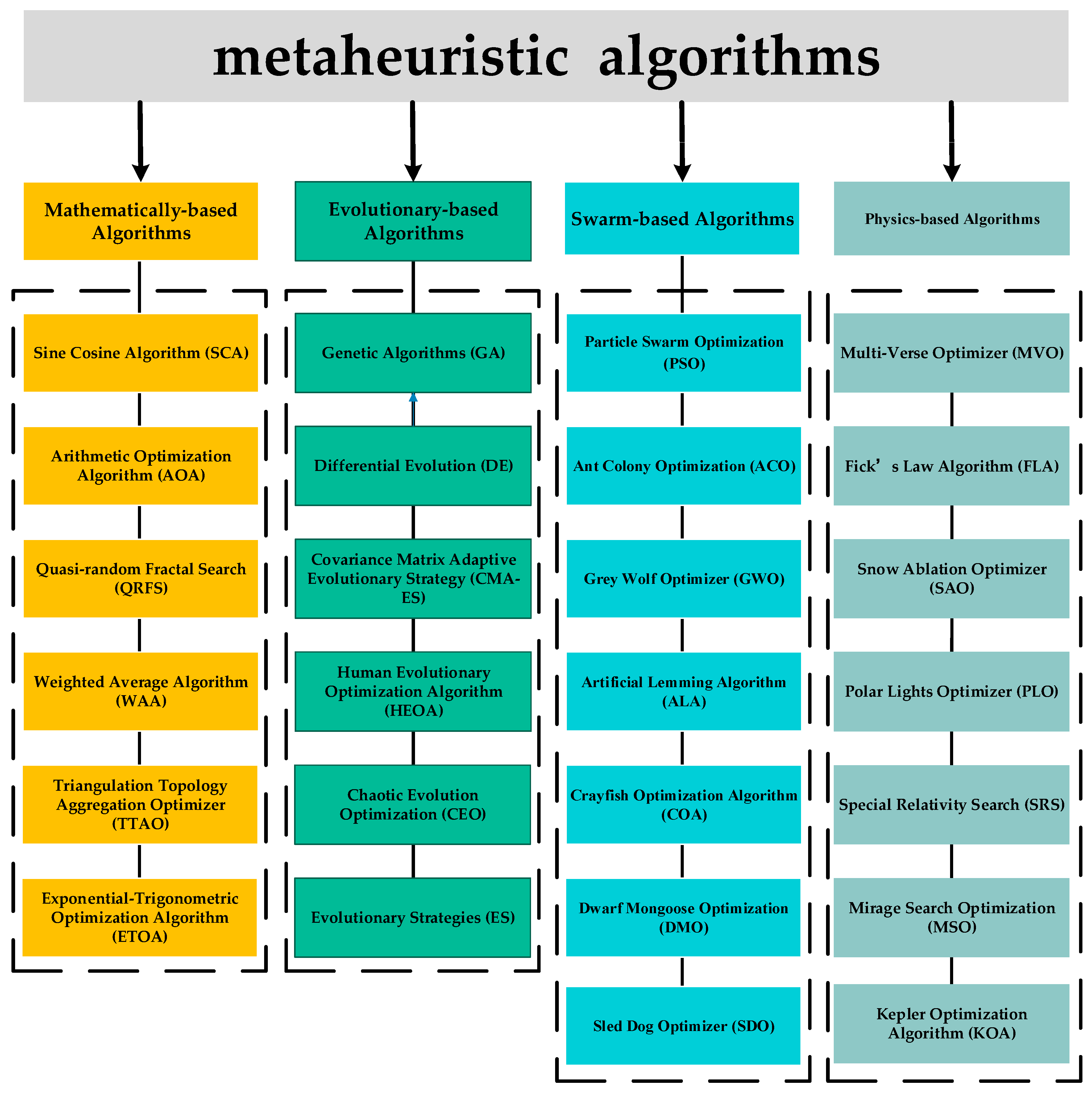
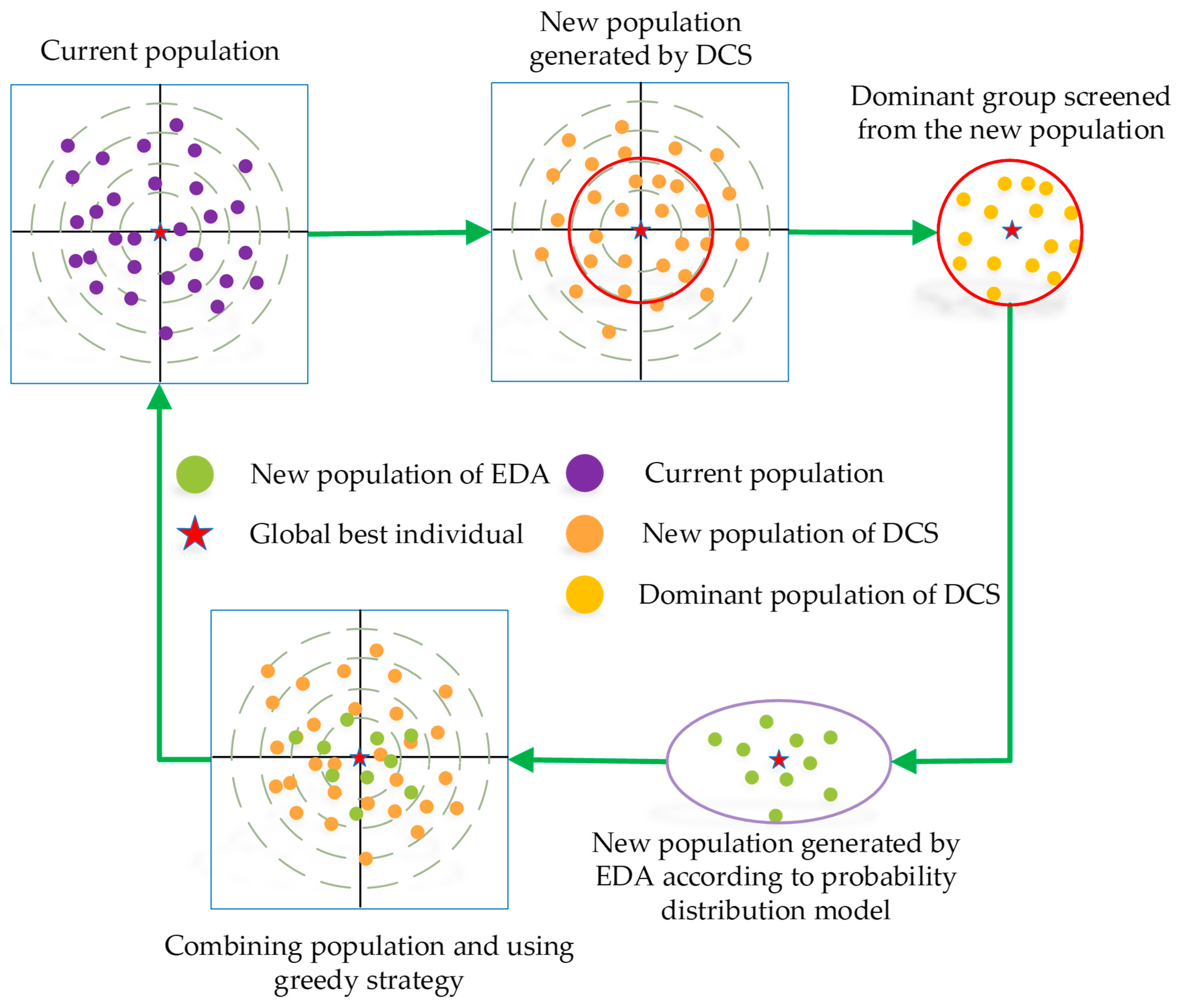


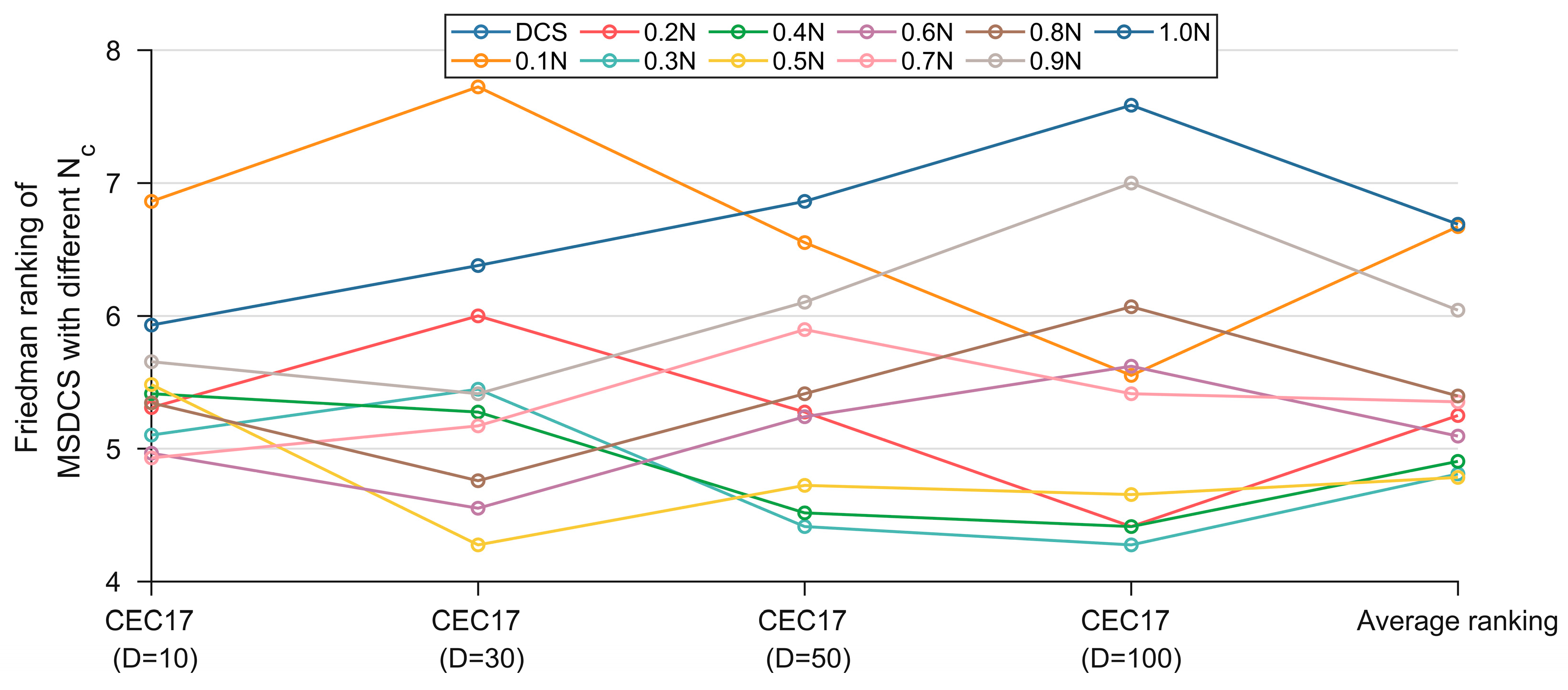
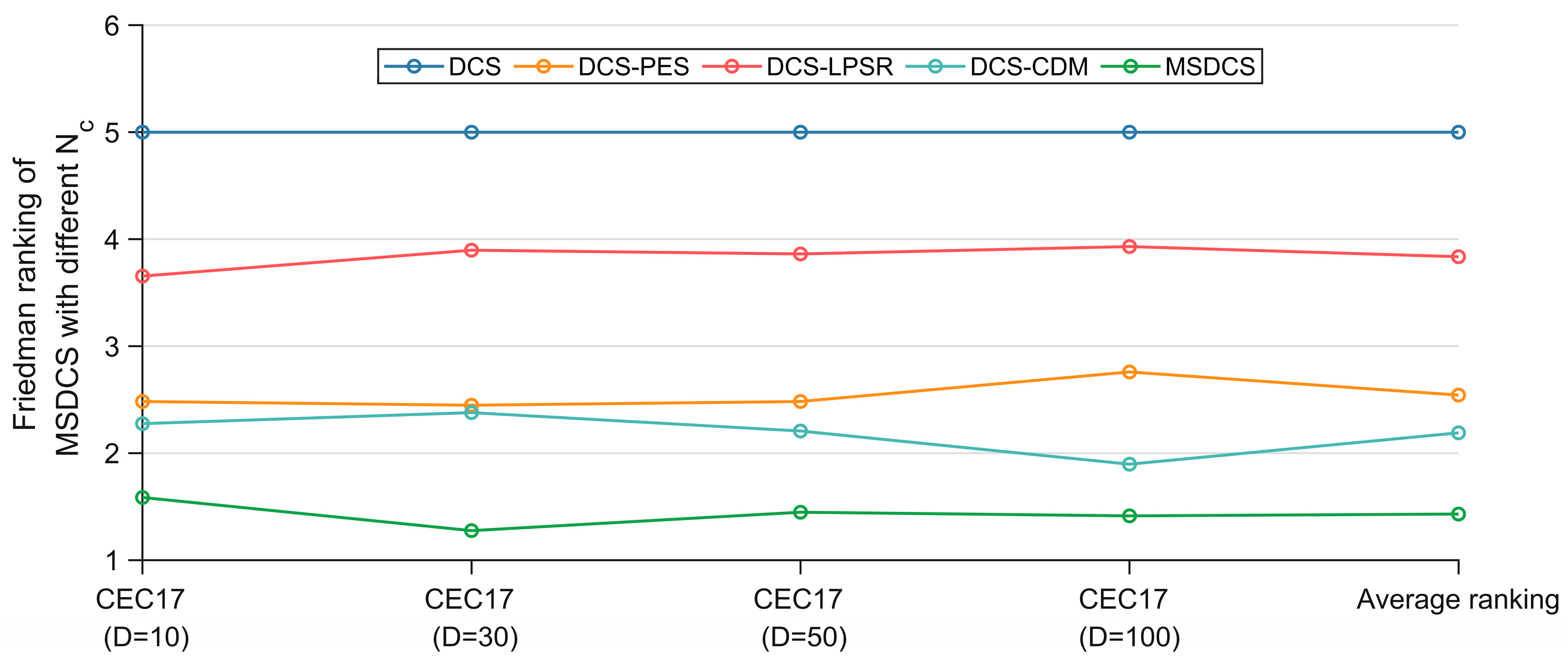

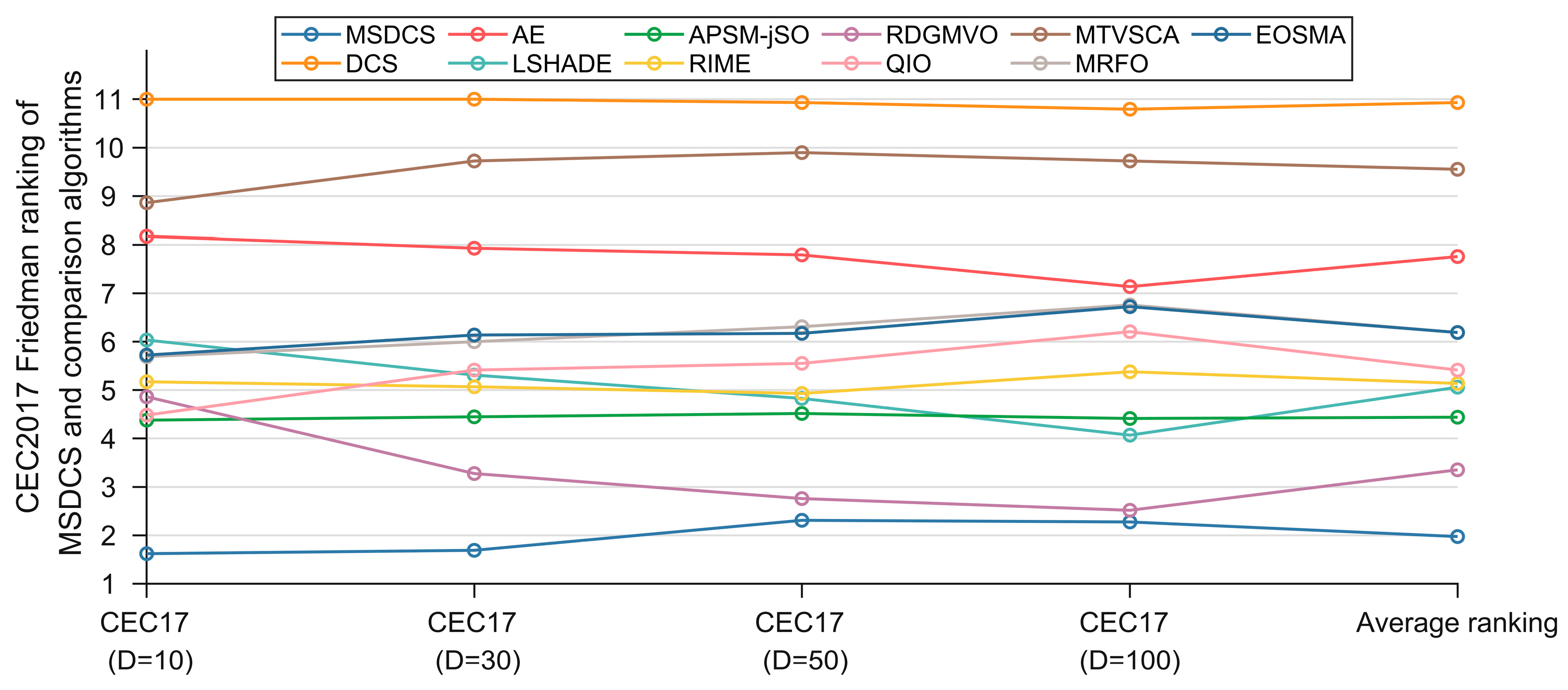

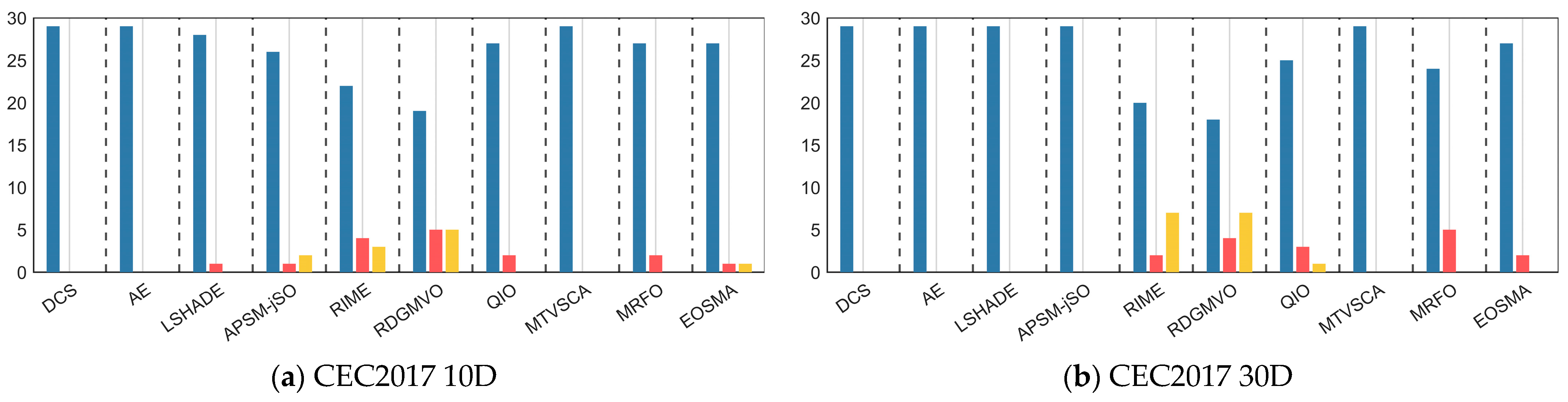

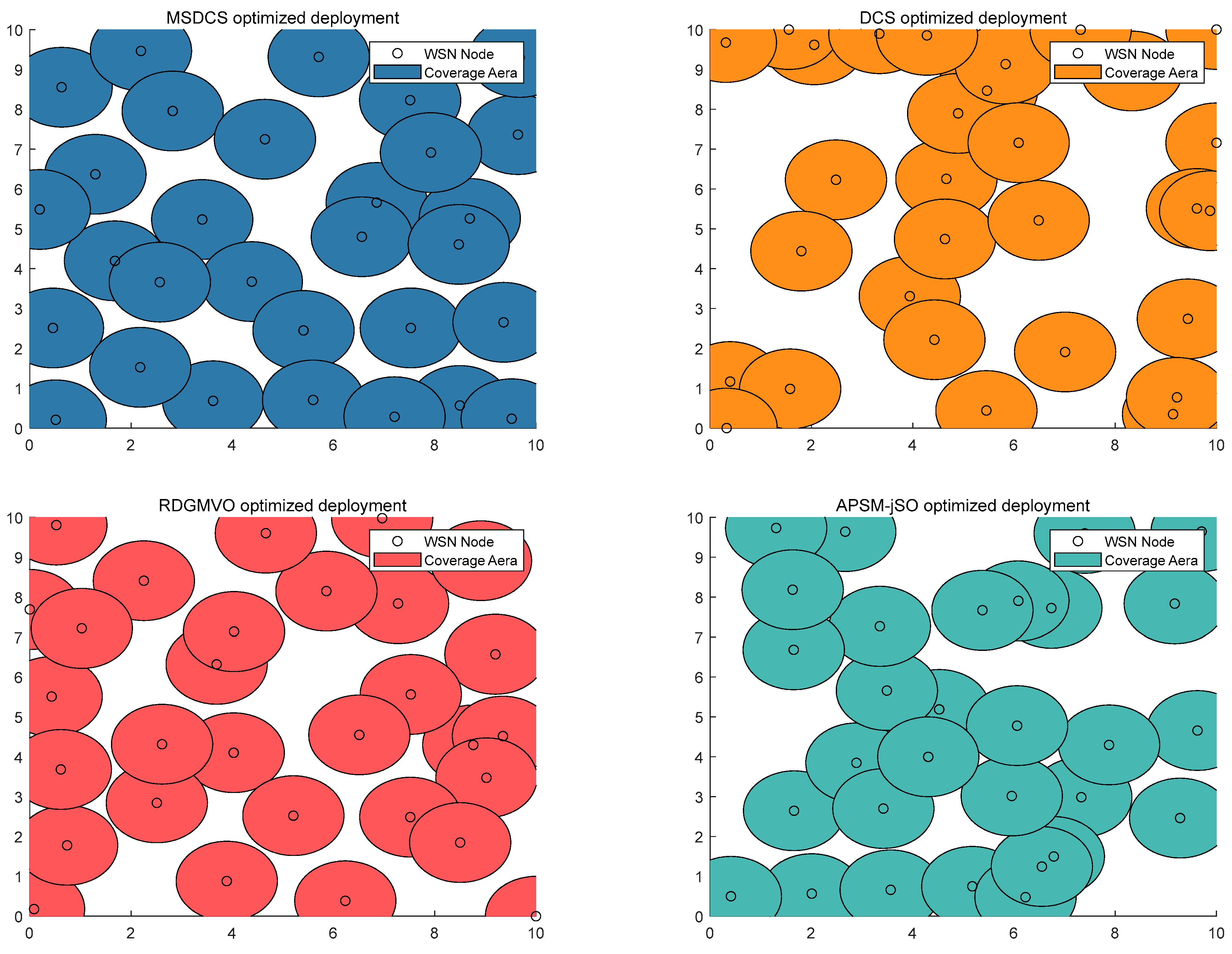
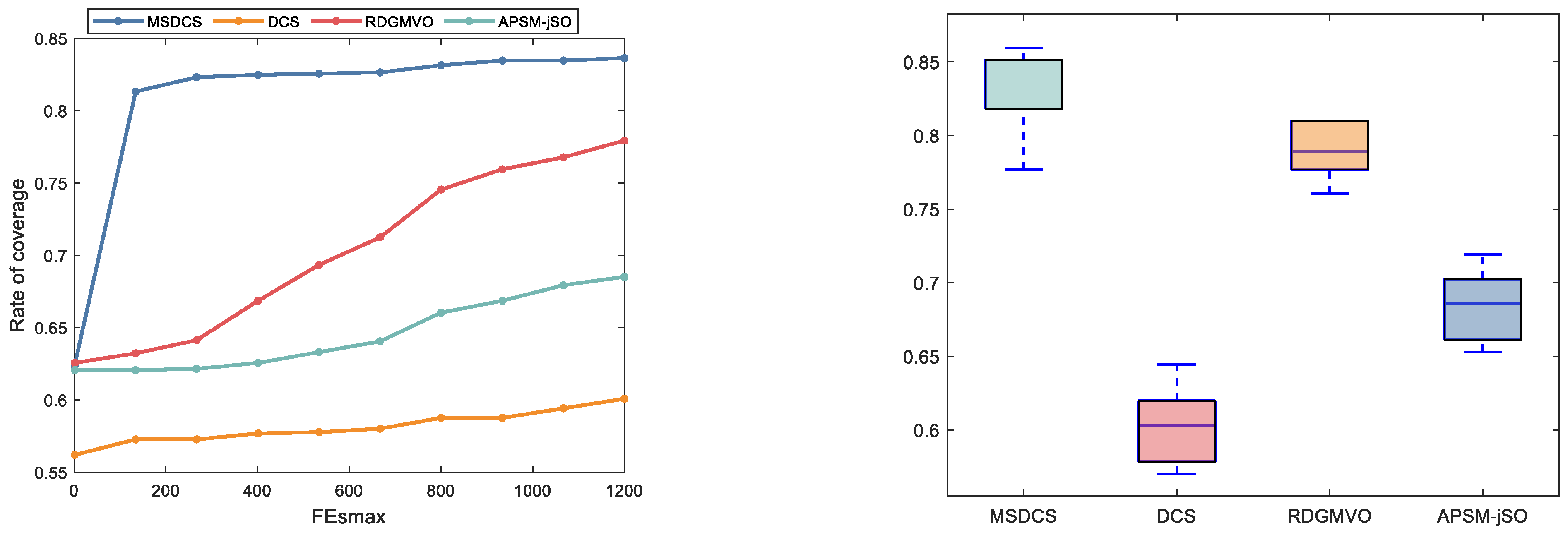

| Algorithm | Parameters Setting |
|---|---|
| MSDCS | |
| DCS | |
| AE [57] | |
| LSHADE [58] | |
| APSM-jSO [59] | |
| RIME [60] | |
| RDGMVO [61] | |
| QIO [62] | |
| MTVSCA [63] | |
| MRFO [64] | |
| EOSMA [65] |
| Dimension | DCS | 0.1N | 0.2N | 0.3N | 0.4N | 0.5N | 0.6N | 0.7N | 0.8N | 0.9N |
|---|---|---|---|---|---|---|---|---|---|---|
| D = 10 | 10.000 | 2.379 | 2.379 | 2.897 | 4.172 | 4.552 | 5.966 | 6.586 | 7.310 | 7.759 |
| D = 30 | 10.000 | 1.931 | 1.931 | 2.241 | 3.379 | 5.069 | 5.897 | 6.828 | 8.103 | 8.621 |
| D = 50 | 10.000 | 1.828 | 1.828 | 2.517 | 3.759 | 4.931 | 5.621 | 7.000 | 7.690 | 8.828 |
| D = 100 | 10.000 | 1.931 | 1.931 | 2.621 | 3.345 | 4.724 | 5.655 | 6.966 | 8.069 | 8.759 |
| Average ranking | 10.000 | 2.017 | 2.017 | 2.569 | 3.664 | 4.819 | 5.784 | 6.845 | 7.793 | 8.491 |
| Dimension | DCS | 0.1N | 0.2N | 0.3N | 0.4N | 0.5N | 0.6N | 0.7N | 0.8N | 0.9N | 0.10N |
|---|---|---|---|---|---|---|---|---|---|---|---|
| D = 10 | 11.000 | 6.862 | 5.310 | 5.103 | 5.414 | 5.483 | 4.966 | 4.931 | 5.345 | 5.655 | 5.931 |
| D = 30 | 11.000 | 7.724 | 6.000 | 5.448 | 5.276 | 4.276 | 4.552 | 5.172 | 4.759 | 5.414 | 6.379 |
| D = 50 | 11.000 | 6.552 | 5.276 | 4.414 | 4.517 | 4.724 | 5.241 | 5.897 | 5.414 | 6.103 | 6.862 |
| D = 100 | 11.000 | 5.552 | 4.414 | 4.276 | 4.414 | 4.655 | 5.621 | 5.414 | 6.069 | 7.000 | 7.586 |
| Average ranking | 11.000 | 6.672 | 5.250 | 4.810 | 4.905 | 4.784 | 5.095 | 5.353 | 5.397 | 6.043 | 6.690 |
| Strategy | DCS | DCS-PES | DCS-LPSR | DCS-CDM | MSDCS |
|---|---|---|---|---|---|
| PES | No | Yes | No | No | Yes |
| LPSR | No | No | Yes | No | Yes |
| CDM | No | No | No | Yes | Yes |
| Test suite | Dimension | DCS | DCS-PES | DCS-LPSR | DCS-CDM | MSDCS | p-Value |
|---|---|---|---|---|---|---|---|
| CEC 2017 | 10 | 5.000 | 2.483 | 3.655 | 2.276 | 1.586 | 2.79E-17 |
| 30 | 5.000 | 2.448 | 3.897 | 2.379 | 1.276 | 2.37E-20 | |
| 50 | 5.000 | 2.483 | 3.862 | 2.207 | 1.448 | 2.55E-19 | |
| 100 | 5.000 | 2.759 | 3.931 | 1.897 | 1.414 | 7.92E-21 | |
| Average ranking | 5.000 | 2.543 | 3.836 | 2.190 | 1.431 | N/A | |
| Ranking | 5 | 3 | 4 | 2 | 1 | N/A | |
| Algorithm | CEC-2017 Test Suite | |||||
|---|---|---|---|---|---|---|
| 10D | 30D | 50D | 100D | Average Ranking | Rank | |
| MSDCS | 1.621 | 1.690 | 2.310 | 2.276 | 1.974 | 1 |
| DCS | 11.000 | 11.000 | 10.931 | 10.793 | 10.931 | 11 |
| AE | 8.172 | 7.931 | 7.793 | 7.138 | 7.759 | 9 |
| LSHADE | 6.034 | 5.310 | 4.828 | 4.069 | 5.060 | 4 |
| APSM-jSO | 4.379 | 4.448 | 4.517 | 4.414 | 4.440 | 3 |
| RIME | 5.172 | 5.069 | 4.931 | 5.379 | 5.138 | 5 |
| RDGMVO | 4.862 | 3.276 | 2.759 | 2.517 | 3.353 | 2 |
| QIO | 4.483 | 5.414 | 5.552 | 6.207 | 5.414 | 6 |
| MTVSCA | 8.862 | 9.724 | 9.897 | 9.724 | 9.552 | 10 |
| MRFO | 5.690 | 6.000 | 6.310 | 6.759 | 6.190 | 7 |
| EOSMA | 5.724 | 6.138 | 6.172 | 6.724 | 6.190 | 7 |
| Friedman P-value | 4.10E-31 | 8.69E-36 | 2.49E-35 | 2.39E-35 | N/A | N/A |
| MSDCS vs. | 10D (+/=/−) | 30D (+/=/−) | 50D (+/=/−) | 100D (+/=/−) | Total (+/=/−) |
|---|---|---|---|---|---|
| DCS | 29/0/0 | 29/0/0 | 29/0/0 | 29/0/0 | 116/0/0 |
| AE | 29/0/0 | 29/0/0 | 29/0/0 | 29/0/0 | 116/0/0 |
| LSHADE | 28/1/0 | 29/0/0 | 29/0/0 | 22/7/0 | 108/8/0 |
| APSM-jSO | 26/1/2 | 29/0/0 | 28/0/1 | 27/1/1 | 108/2/4 |
| RIME | 22/4/3 | 20/2/7 | 18/2/9 | 20/0/9 | 80/8/28 |
| RDGMVO | 19/5/5 | 18/4/7 | 12/3/14 | 13/4/12 | 62/16/38 |
| QIO | 27/2/0 | 25/3/1 | 23/3/3 | 26/1/2 | 101/9/6 |
| MTVSCA | 29/0/0 | 29/0/0 | 29/0/0 | 29/0/0 | 116/0/0 |
| MRFO | 27/2/0 | 24/5/0 | 23/2/4 | 24/0/5 | 95/9/9 |
| EOSMA | 27/1/1 | 27/2/0 | 25/1/3 | 25/1/3 | 104/5/7 |
| Algorithm | Best | Mean | Std |
| MSDCS | 85.95% | 83.64% | 0.026 |
| DCS | 64.46% | 60.08% | 0.025 |
| RDGMVO | 80.99% | 78.93% | 0.018 |
| APSM-jSO | 71.90% | 68.51% | 0.022 |
| Problem | Name | D |
|---|---|---|
| CE01 | Tension/compression spring design problem | 3 |
| CE02 | Pressure vessel design problem | 4 |
| CE03 | Three-bar truss design problem | 2 |
| CE04 | Welded beam design problem | 4 |
| CE05 | Speed reducer design problem | 7 |
| CE06 | Gear train design problem | 4 |
| CE07 | Rolling element bearing design | 10 |
| CE08 | Cantilever beam design problem | 5 |
| CE09 | Multiple disk clutch brake design problem | 5 |
| CE10 | Step-cone pulley problem | 5 |
| Function | Index | MSDCS | DCS | AE | LSHADE | APSM-jSO | RIME | RDGMVO | QIO | MTVSCA | MRFO | EOSMA |
|---|---|---|---|---|---|---|---|---|---|---|---|---|
| CE1 | Best | 1.2671E-02 | 2.4083E-02 | 1.3191E-02 | 1.2907E-02 | 1.2871E-02 | 1.3529E-02 | 1.3044E-02 | 1.2921E-02 | 1.3906E-02 | 1.3057E-02 | 1.2846E-02 |
| Mean | 1.2860E-02 | 7.3531E+03 | 1.4128E-02 | 1.3296E-02 | 1.3054E-02 | 1.6235E-02 | 1.3356E-02 | 1.3383E-02 | 1.6551E-02 | 1.3777E-02 | 1.3695E-02 | |
| Std | 2.8359E-04 | 1.6442E+04 | 1.0954E-03 | 3.2821E-04 | 1.4931E-04 | 2.9673E-03 | 4.1936E-04 | 4.1607E-04 | 2.4984E-03 | 7.4353E-04 | 9.4204E-04 | |
| Rank | 1 | 11 | 8 | 3 | 2 | 9 | 4 | 5 | 10 | 7 | 6 | |
| CE2 | Best | 5.8701E+03 | 1.7715E+05 | 6.6293E+03 | 6.3630E+03 | 6.0647E+03 | 6.0556E+03 | 7.6793E+03 | 6.3236E+03 | 1.2028E+04 | 6.5909E+03 | 7.1900E+03 |
| Mean | 5.9511E+03 | 3.2762E+05 | 8.0280E+03 | 6.5037E+03 | 6.5380E+03 | 6.9088E+03 | 8.3425E+03 | 6.8454E+03 | 1.3060E+04 | 7.0169E+03 | 8.3431E+03 | |
| Std | 1.6259E+02 | 1.9473E+05 | 1.1292E+03 | 2.4059E+02 | 4.8136E+02 | 7.6999E+02 | 1.1312E+03 | 3.2487E+02 | 1.1049E+03 | 5.8863E+02 | 1.0649E+03 | |
| Rank | 1 | 11 | 7 | 2 | 3 | 5 | 8 | 4 | 10 | 6 | 9 | |
| CE3 | Best | 2.6389E+02 | 2.6395E+02 | 2.6391E+02 | 2.6390E+02 | 2.6390E+02 | 2.6394E+02 | 2.6389E+02 | 2.6389E+02 | 2.6405E+02 | 2.6389E+02 | 2.6390E+02 |
| Mean | 2.6389E+02 | 2.6468E+02 | 2.6393E+02 | 2.6390E+02 | 2.6392E+02 | 2.6442E+02 | 2.6394E+02 | 2.6390E+02 | 2.6433E+02 | 2.6394E+02 | 2.6402E+02 | |
| Std | 2.8422E-14 | 1.0184E+00 | 1.4357E-02 | 5.1566E-03 | 2.7481E-02 | 7.0931E-01 | 5.5071E-02 | 2.6617E-03 | 2.9947E-01 | 4.1346E-02 | 1.6598E-01 | |
| Rank | 1 | 11 | 5 | 3 | 4 | 10 | 7 | 2 | 9 | 6 | 8 | |
| CE4 | Best | 1.6928E+00 | 2.2522E+00 | 1.8755E+00 | 1.7093E+00 | 1.7255E+00 | 1.7528E+00 | 1.8060E+00 | 1.7362E+00 | 1.8941E+00 | 1.7390E+00 | 1.7520E+00 |
| Mean | 1.6928E+00 | 3.1607E+00 | 1.9597E+00 | 1.7362E+00 | 1.7744E+00 | 1.9554E+00 | 1.9708E+00 | 1.7493E+00 | 2.0044E+00 | 1.7759E+00 | 1.8056E+00 | |
| Std | 6.0366E-07 | 7.2634E-01 | 5.6745E-02 | 2.1821E-02 | 7.5693E-02 | 2.3237E-01 | 2.3252E-01 | 1.4943E-02 | 8.2997E-02 | 4.0763E-02 | 4.0271E-02 | |
| Rank | 1 | 11 | 8 | 2 | 4 | 7 | 9 | 3 | 10 | 5 | 6 | |
| CE5 | Best | 2.9936E+03 | 3.1674E+03 | 2.8842E+03 | 2.9955E+03 | 2.9937E+03 | 3.0006E+03 | 3.0000E+03 | 3.0179E+03 | 3.0581E+03 | 3.0126E+03 | 3.0136E+03 |
| Mean | 2.9936E+03 | 3.6127E+03 | 2.9817E+03 | 2.9964E+03 | 2.9937E+03 | 3.0081E+03 | 3.0054E+03 | 3.0395E+03 | 3.0836E+03 | 3.0205E+03 | 3.0196E+03 | |
| Std | 1.2705E-08 | 5.4941E+02 | 8.1403E+01 | 5.7719E-01 | 4.6451E-02 | 1.4537E+01 | 3.5675E+00 | 1.7883E+01 | 2.8303E+01 | 6.8185E+00 | 4.7228E+00 | |
| Rank | 2 | 11 | 1 | 4 | 3 | 6 | 5 | 9 | 10 | 8 | 7 | |
| CE6 | Best | 2.7009E-12 | 6.5257E-08 | 2.7009E-12 | 2.7009E-12 | 2.7009E-12 | 2.3078E-11 | 3.0676E-10 | 2.7009E-12 | 9.7457E-10 | 2.3078E-11 | 2.3078E-11 |
| Mean | 2.5107E-10 | 2.9280E-04 | 1.6136E-09 | 1.3787E-09 | 1.8025E-09 | 1.6091E-09 | 1.8218E-09 | 6.9316E-10 | 1.5824E-08 | 1.0321E-09 | 1.4391E-09 | |
| Std | 5.2127E-10 | 2.6088E-04 | 1.0773E-09 | 9.9970E-10 | 2.8168E-09 | 1.6964E-09 | 1.6550E-09 | 6.3136E-10 | 3.1042E-08 | 9.6274E-10 | 1.2581E-09 | |
| Rank | 1 | 11 | 7 | 4 | 8 | 6 | 9 | 2 | 10 | 3 | 5 | |
| CE7 | Best | -2.4358E+05 | -1.2042E+05 | -1.1897E+03 | -2.4358E+05 | -2.4358E+05 | -2.4358E+05 | -2.4358E+05 | -2.3030E+05 | -2.2659E+05 | -2.3612E+05 | -2.4144E+05 |
| Mean | -2.4358E+05 | 1.5159E+06 | -1.0860E+03 | -2.4356E+05 | -2.4358E+05 | -2.4314E+05 | -2.4358E+05 | -2.2349E+05 | -2.2243E+05 | -2.3002E+05 | -2.4025E+05 | |
| Std | 5.8147E-07 | 1.8087E+06 | 5.8056E+01 | 2.7780E+01 | 1.2992E-09 | 4.4409E+02 | 5.3962E+00 | 8.2081E+03 | 4.6563E+03 | 7.9789E+03 | 8.0731E+02 | |
| Rank | 2 | 11 | 10 | 4 | 1 | 5 | 3 | 8 | 9 | 7 | 6 | |
| CE8 | Best | 1.3400E+00 | 2.0342E+00 | 1.4263E+00 | 1.3467E+00 | 1.3511E+00 | 1.3525E+00 | 1.4144E+00 | 1.3409E+00 | 1.4359E+00 | 1.3426E+00 | 1.3554E+00 |
| Mean | 1.3400E+00 | 3.1656E+00 | 1.4467E+00 | 1.3601E+00 | 1.3577E+00 | 1.4106E+00 | 1.6551E+00 | 1.3430E+00 | 1.5526E+00 | 1.3496E+00 | 1.3609E+00 | |
| Std | 1.2511E-07 | 1.1175E+00 | 1.9849E-02 | 1.4979E-02 | 7.8764E-03 | 4.2675E-02 | 2.0798E-01 | 2.9635E-03 | 9.4868E-02 | 9.2797E-03 | 4.3679E-03 | |
| Rank | 1 | 11 | 8 | 5 | 4 | 7 | 10 | 2.0000E+00 | 9.0000E+00 | 3.0000E+00 | 6.0000E+00 | |
| CE9 | Best | 3.9247E+08 | 3.9247E+08 | 2.5199E+08 | 3.9247E+08 | 3.9247E+08 | 3.9247E+08 | 3.9247E+08 | 3.9247E+08 | 3.9247E+08 | 3.9247E+08 | 3.9247E+08 |
| Mean | 3.9247E+08 | 3.9474E+08 | 2.5245E+08 | 3.9247E+08 | 3.9247E+08 | 3.9247E+08 | 3.9247E+08 | 3.9247E+08 | 3.9247E+08 | 3.9247E+08 | 3.9247E+08 | |
| Std | 0.0000E+00 | 4.5209E+06 | 8.8091E+05 | 0.0000E+00 | 0.0000E+00 | 0.0000E+00 | 0.0000E+00 | 9.2258E-02 | 1.8781E+03 | 3.4870E-01 | 0.0000E+00 | |
| Rank | 2 | 11 | 1 | 2 | 2 | 2 | 2 | 8 | 10 | 9 | 2 | |
| CE10 | Best | 1.6086E+01 | 1.7337E+04 | 2.2769E+01 | 1.7146E+01 | 1.6594E+01 | 1.6282E+01 | 1.6886E+01 | 1.6576E+01 | 7.8319E+01 | 1.6735E+01 | 1.7144E+01 |
| Mean | 1.6086E+01 | 7.0920E+08 | 8.0915E+01 | 1.7397E+01 | 1.7053E+01 | 1.6967E+01 | 1.9526E+01 | 1.6696E+01 | 1.4682E+02 | 1.7109E+01 | 1.7557E+01 | |
| Std | 4.8761E-07 | 1.3571E+09 | 1.0977E+02 | 3.2555E-01 | 4.5030E-01 | 5.6418E-01 | 3.9405E+00 | 1.1886E-01 | 7.2506E+01 | 3.1909E-01 | 4.4901E-01 | |
| Rank | 1 | 11 | 9 | 6 | 4 | 3 | 8 | 2 | 10 | 5 | 7 |
Disclaimer/Publisher’s Note: The statements, opinions and data contained in all publications are solely those of the individual author(s) and contributor(s) and not of MDPI and/or the editor(s). MDPI and/or the editor(s) disclaim responsibility for any injury to people or property resulting from any ideas, methods, instructions or products referred to in the content. |
© 2025 by the authors. Licensee MDPI, Basel, Switzerland. This article is an open access article distributed under the terms and conditions of the Creative Commons Attribution (CC BY) license (https://creativecommons.org/licenses/by/4.0/).
Share and Cite
Cai, X.; Zhang, C. An Innovative Differentiated Creative Search Based on Collaborative Development and Population Evaluation. Biomimetics 2025, 10, 260. https://doi.org/10.3390/biomimetics10050260
Cai X, Zhang C. An Innovative Differentiated Creative Search Based on Collaborative Development and Population Evaluation. Biomimetics. 2025; 10(5):260. https://doi.org/10.3390/biomimetics10050260
Chicago/Turabian StyleCai, Xinyu, and Chaoyong Zhang. 2025. "An Innovative Differentiated Creative Search Based on Collaborative Development and Population Evaluation" Biomimetics 10, no. 5: 260. https://doi.org/10.3390/biomimetics10050260
APA StyleCai, X., & Zhang, C. (2025). An Innovative Differentiated Creative Search Based on Collaborative Development and Population Evaluation. Biomimetics, 10(5), 260. https://doi.org/10.3390/biomimetics10050260