Speed Responses to Speed Humps as Affected by Time of Day and Light Conditions on a Residential Road with Light-Emitting Diode (LED) Road Lighting


Abstract
:1. Introduction
- (I)
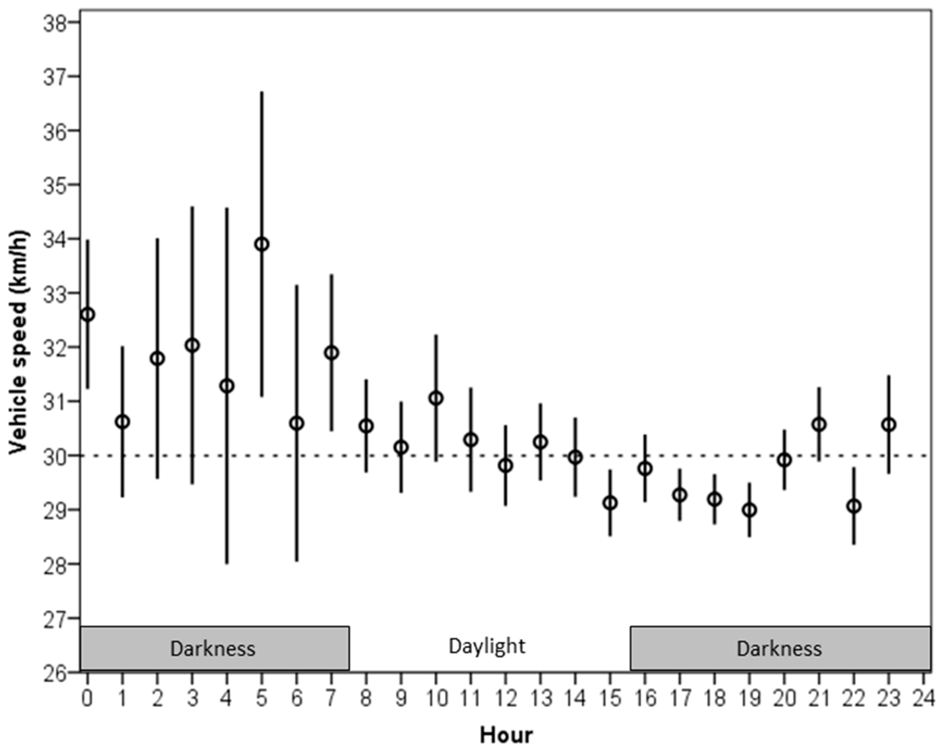
- Vehicle speed is higher during daylight than in darkness.
- (II)
- Vehicle speed at speed humps is lower than at control locations during both daylight and darkness.
- (III)
- Speed at humps is higher during daylight.
- (IV)
- Speed at humps is lower when luminance (visibility) of the humps is greater.
- (V)
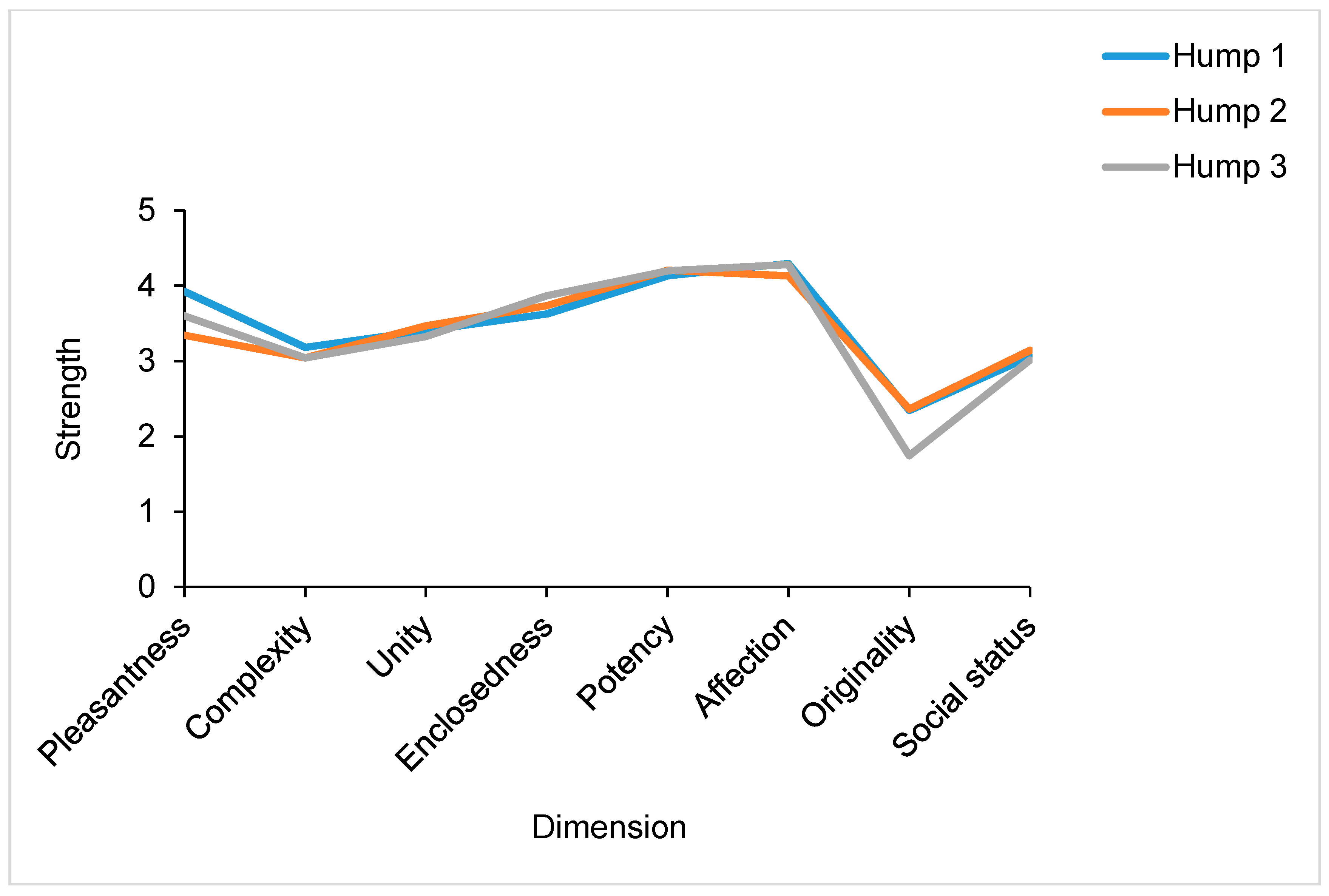
- The road environment of speed humps is perceived as being similar by drivers.
2. Materials and Methods
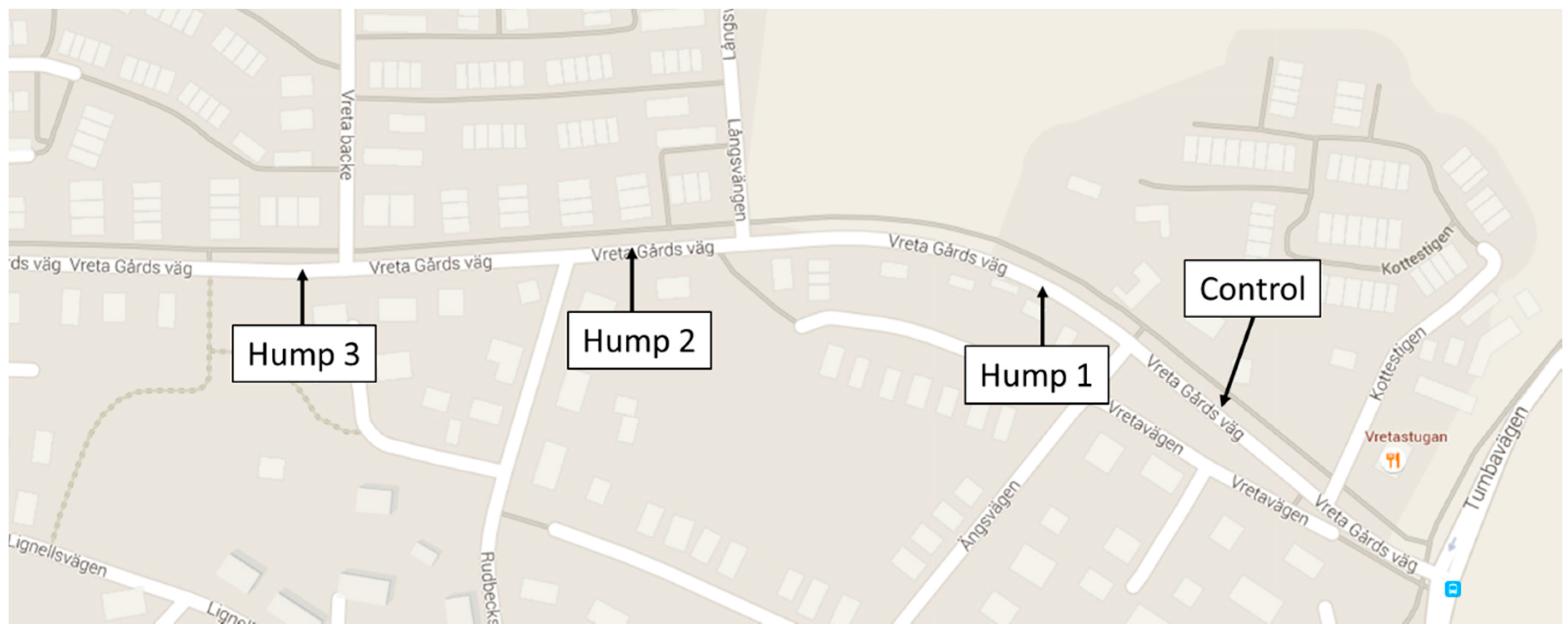
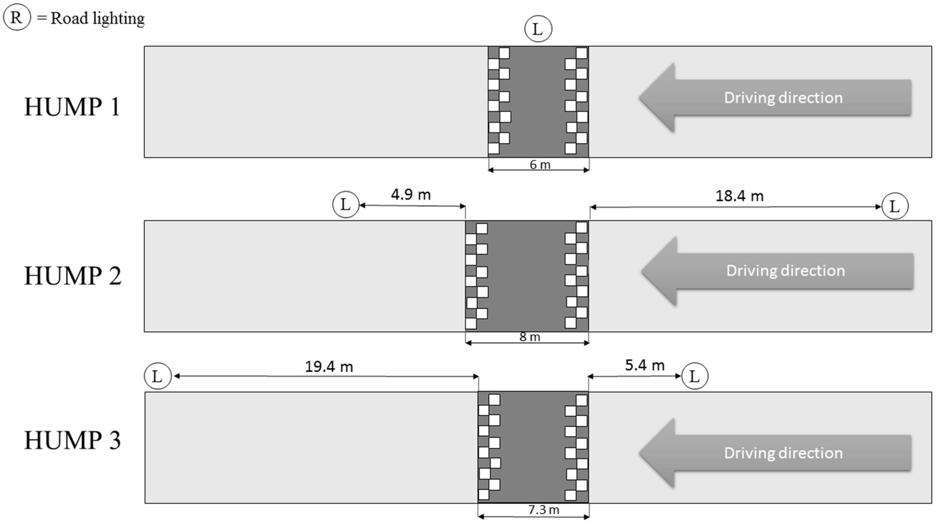
2.1. Site Description
2.2. Experimental Design and Speed Measurements
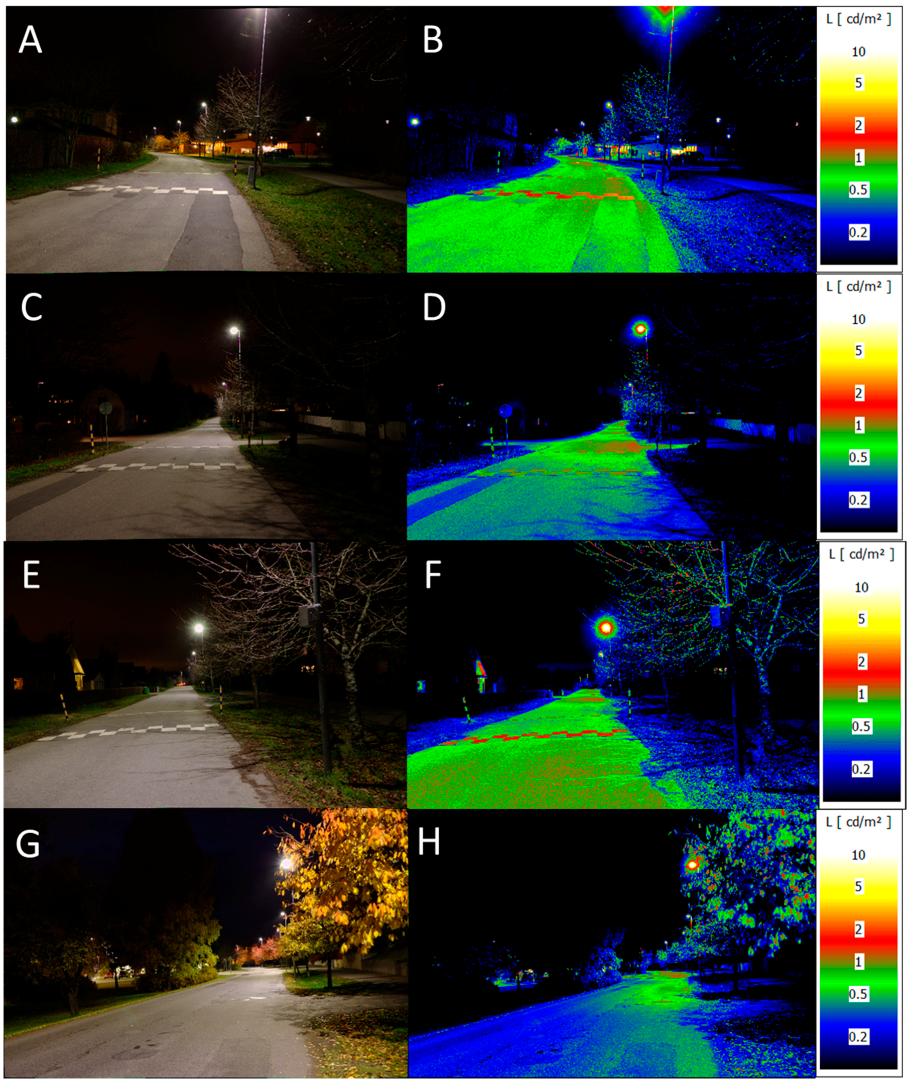
2.3. Road Lighting and Light Measurements
2.4. Semantic Description of Environments
2.5. Data Analyses
3. Results
4. Discussion
5. Conclusions
Supplementary Materials
Acknowledgments
Author Contributions
Conflicts of Interest
References
- Johansson, R. Vision zero—Implementing a policy for traffic safety. Saf. Sci. 2009, 47, 826–831. [Google Scholar] [CrossRef]
- Anderson, R.W.G.; McLean, A.J.; Farmer, M.J.B.; Lee, B.H.; Brooks, C.G. Vehicle travel speeds and the incidence of fatal pedestrian crashes. Accid. Anal. Prev. 1997, 29, 667–674. [Google Scholar] [CrossRef]
- Rosén, E.; Stigson, H.; Sander, U. Literature review of pedestrian fatality risk as a function of car impact speed. Accid. Anal. Prev. 2011, 43, 25–33. [Google Scholar] [CrossRef] [PubMed]
- Pau, M.; Angius, S. Do speed bumps really decrease traffic speed? An italian experience. Accid. Anal. Prev. 2001, 33, 585–597. [Google Scholar] [CrossRef]
- Johnson, L.; Nedzesky, A.J. A Comparative Study of Speed Humps, Speed Slots and Speed Cushions; U.S. Department of Transportation, Federal Highway Administration, Report. 2004. Available online: http://safety.fhwa.dot.gov/speedmgt/ref_mats/fhwasa1304/Resources3/26%20-%20A%20Comparative%20Study%20of%20Speed%20Humps,%20Speed%20Slots%20and%20Speed%20Cushions.pdf (accessed on 21 December 2017).
- ITE. Traffic Calming Measures—Speed Hump. Available online: http://www.ite.org/traffic/hump.asp (accessed on 31 December 2017).
- Bassani, M.; Dalmazzo, D.; Riviera, P.P. Field Investigation on the Effects on Operating Speed Caused by trapezoidal humps. In Proceedings of the Transportation Research Board 90th Annual Meeting, Washington, DC, USA, 23–27 January 2011; Transportation Research Board: Washington, DC, USA, 2011. [Google Scholar]
- Hallmark, S.; Knapp, K.; Thomas, G.; Smith, D. Temporary Speed Hump Impact Evaluation; CTRE Project 00-73; Centre for Transportation Research and Education, Iowa State University: Ames, IA, USA, 2002. [Google Scholar]
- Sumner, R.; Baguley, C. Speed Control Humps on Residential Roads; TRRL Laboratory Report 878; Transport and Road Research Laboratory: Wokingham, UK, 1979. [Google Scholar]
- Barbosa, H.M.; Tight, M.R.; May, A.D. A model of speed profiles for traffic calmed roads. Transp. Res. Part A 2000, 34, 103–123. [Google Scholar] [CrossRef]
- Salau, T.A.O.; Adeyefa, A.O.; Oke, S.A. Vehicle speed control using road bumps. Transport 2004, 19, 130–136. [Google Scholar]
- Molan, A.M.; Kordani, A.A. Optimization of speed hump profiles based on vehicle dynamic performance modeling. J. Transp. Eng. 2014, 140, 04014035. [Google Scholar] [CrossRef]
- Tester, J.M.; Rutherford, G.W.; Wald, Z.; Rutherford, M.W. A matched case-control study evaluating the effectiveness of speed humps in reducing child pedestrian injuries. Am. J. Public Health 2004, 94, 646–650. [Google Scholar] [CrossRef] [PubMed]
- Rothman, L.; Macpherson, A.; Buliung, R.; Macarthur, C.; To, T.; Larsen, K.; Howard, A. Installation of speed humps and pedestrian-motor vehicle collisions in toronto, canada: A quasi-experimental study. BMC Public Health 2015, 15, 774. [Google Scholar] [CrossRef] [PubMed]
- Elvik, R. Meta-analysis of evaluations of public lighting as accident countermeasure. Transp. Res. Rec. 1995, 1485, 112–123. Available online: http://onlinepubs.trb.org/Onlinepubs/trr/1995/1485/1485-015.pdf (accessed on 9 March 2018).
- Johansson, O.; Wanvik, P.O.; Elvik, R. A new method for assessing the risk of accident associated with darkness. Accid. Anal. Prev. 2009, 41, 809–815. [Google Scholar] [CrossRef] [PubMed]
- Wanvik, P.O. Effects of road lighting: An analysis based on dutch accident statistics 1987–2006. Accid. Anal. Prev. 2009, 41, 123–128. [Google Scholar] [CrossRef] [PubMed]
- Beyer, F.R.; Ker, K. Street lighting for preventing road traffic injuries. Cochrane Database Syst. Rev. 2009. [Google Scholar] [CrossRef] [PubMed]
- Sullivan, J.M.; Flannagan, M.J. Determining the potential safety benefit of improved lighting in three pedestrian crash scenarios. Accid. Anal. Prev. 2007, 39, 638–647. [Google Scholar] [CrossRef] [PubMed]
- Elvik, R.; Vaa, T. The Handbook of Road Safety Measures; Emerald Group Publishing Limited: Bingley, UK, 2004. [Google Scholar]
- Monsere, C.M.; Fischer, E.L. Safety effects of reducing freeway illumination for energy conservation. Accid. Anal. Prev. 2008, 40, 1773–1780. [Google Scholar] [CrossRef] [PubMed]
- Möller, S. Väglag-Trafikflöde-Hastighet. En Studie av Nyttan Med att ta Hänsyn till Väglaget vid Bortfallskomplettering av Trafikflöde och Hastighet; VTI Meddelande 794; The Swedish National Road and Transport Research Institute: Linköping, Sweden, 1996; pp. 1–37.
- Assum, T.; Bjørnskau, T.; Fosser, S.; Sagberg, F. Risk compensation—The case of road lighting. Accid. Anal. Prev. 1999, 31, 545–553. [Google Scholar] [CrossRef]
- Bassani, M.; Mutani, G. Effects of environmental lighting conditions on operating speeds on urban arterials. Transp. Res. Rec. 2012, 2298, 78–87. [Google Scholar] [CrossRef]
- Quaium, R.B.A. A Comparison of Vehicle Speed at Day and Night at Rural Horizontal Curves. Master’s Thesis, Virginia Polytechnic Institute and State University, Blacksburg, VA, USA, 2010. [Google Scholar]
- Jägerbrand, A.K.; Sjöbergh, J. Effects of weather conditions, light conditions, and road lighting on vehicle speed. SpringerPlus 2016, 5, 505. [Google Scholar] [CrossRef] [PubMed]
- Jägerbrand, A.K. New framework of sustainable indicators for outdoor led (light emitting diodes) lighting and ssl (solid state lighting). Sustainability 2015, 7, 1028–1063. [Google Scholar] [CrossRef]
- Kuhn, L.; Johansson, M.; Laike, T.; Govén, T. Residents perceptions following retrofitting of residential area outdoor lighting with leds. Light. Res. Technol. 2013, 45, 568–584. [Google Scholar] [CrossRef]
- Tashiro, T.; Kawanobe, S.; Kimura-Minoda, T.; Kohko, S.; Ishikawa, T.; Ayama, M. Discomfort glare for white led light sources with different spatial arrangements. Light. Res. Technol. 2015, 47, 316–337. [Google Scholar] [CrossRef]
- Küller, R. Semantisk Miljö Beskrivning (SMB); Psykologiförlaget AB, Liber Tryck: Stockholm, Sweden, 1975; pp. 1–44. [Google Scholar]
- Vogel, K. What characterizes a “free vehicle” in an urban area? Transp. Res. Part F 2002, 5, 313–327. [Google Scholar] [CrossRef]
- Bozdogan, H. Model selection and akaike’s information criteria (aic): The general theory and its analytical extensions. Psychometrika 1987, 52, 345–370. [Google Scholar] [CrossRef]
- Leibowitz, H.W.; Owens, D.A.; Tyrrell, R.A. The assured clear distance ahead rule: Implications for nighttime traffic safety and the law. Accid. Anal. Prev. 1998, 30, 93–99. [Google Scholar] [CrossRef]
- Owens, D.A.; Tyrrell, R.A. Effects of luminance, blur, and age on nighttime visual guidance: A test of the selective degradation hypothesis. J. Exp. Psychol. 1999, 5, 115–128. [Google Scholar] [CrossRef]
- Owens, D.A.; Wood, J.M.; Owens, J.M. Effects of age and illumination on night driving: A road test. Hum. Factors 2007, 49, 1115–1131. [Google Scholar] [CrossRef] [PubMed]


| Location and Natural Light Conditions | n | M | SD | 50th Percentile | 85th Percentile |
|---|---|---|---|---|---|
| Control (all) | 4803 | 28.9 | 5.7 | 29.0 | 36.0 |
| Daylight | 1571 | 30.1 | 5.8 | 30.0 | 36.0 |
| Darkness | 3232 | 29.8 | 5.7 | 29.0 | 36.0 |
| Humps (all) | 18252 | 23.7 | 5.4 | 23.0 | 29.0 |
| Daylight | 5392 | 23.8 | 5.4 | 23.0 | 29.0 |
| Darkness | 12860 | 23.6 | 5.4 | 23.0 | 29.0 |
| Model Effects | Type III | ||
|---|---|---|---|
| Source | Wald Chi-Square | df | p |
| Question 1. Is speed higher during daylight at the control location? | |||
| Model: Daylight and darkness + road temperature + precipitation type (n = 4803) | |||
| (Intercept) | 39,161.44 | 1 | <0.001 |
| Daylight and darkness | 4.01 | 1 | 0.045 |
| Road temperature | 0.78 | 1 | 0.377 |
| Precipitation type | 1.66 | 2 | 0.437 |
| Question 2. Is speed at speed humps lower during daylight and in darkness compared with the control location? | |||
| Model: Humps & control + road temperature + precipitation type (n = 6963 daylight; n = 16092 darkness) | |||
| Daylight | |||
| (Intercept) | 24,355.07 | 1 | <0.001 |
| Humps or control | 2527.51 | 3 | <0.001 |
| Road temperature | 11.45 | 1 | 0.001 |
| Precipitation type | 21.18 | 2 | <0.001 |
| Darkness | |||
| (Intercept) | 83,832.64 | 1 | <0.001 |
| Humps or control | 6683.37 | 3 | <0.001 |
| Road temperature | 1.48 | 1 | 0.224 |
| Precipitation type | 20.59 | 2 | <0.001 |
| Question 3. Is the speed-reducing effect of speed humps similar in daylight and darkness? | |||
| Model *: D + RT + P + D × RT + D × P + RT × P (n = 18,252) | |||
| (Intercept) | 40,817.88 | 1 | <0.001 |
| Daylight and darkness (D) | 0.27 | 1 | 0.607 |
| Road temperature (RT) | 3.35 | 1 | 0.067 |
| Precipitation type (P) | 39.98 | 2 | <0.001 |
| D × RT | 10.51 | 1 | 0.001 |
| D × P | 6.13 | 2 | 0.047 |
| RT × P | 0.58 | 1 | 0.445 |
| Question 4. Is the speed-reducing effect of speed humps greater when hump luminance is higher? | |||
| Model: Humps + RT + P (n = 5879) | |||
| (Intercept) | 37,688.45 | 1 | <0.001 |
| Humps | 1351.19 | 2 | <0.001 |
| Road temperature | 1.63 | 1 | 0.201 |
| Precipitation type | 13.40 | 2 | 0.001 |
| Parameter | B | SE | 95% Wald Confidence Interval | Hypothesis Test | |||
|---|---|---|---|---|---|---|---|
| Lower | Upper | Wald Chi-Square | df | p | |||
| Question 1. Is speed higher during daylight at the control location? | |||||||
| Model: Daylight + darkness + road temperature + precipitation type (n = 4803) | |||||||
| (Intercept) | 29.54 | 0.31 | 28.93 | 30.16 | 8805.57 | 1 | <0.001 |
| Daylight | 0.36 | 0.18 | 0.01 | 0.71 | 4.01 | 1 | 0.045 |
| Question 2. Is speed at speed humps lower during daylight and in darkness compared with the control location? | |||||||
| Model: humps and control + road temperature + precipitation type (n = 6963 daylight; n = 16,092 darkness) | |||||||
| Daylight | |||||||
| (Intercept) | 28.96 | 0.28 | 28.42 | 29.50 | 10,911.32 | 1 | <0.001 |
| Hump 1 | −7.21 | 0.17 | −7.53 | −6.88 | 1852.42 | 1 | <0.001 |
| Hump 3 | −7.98 | 0.20 | −8.37 | −7.59 | 1602.65 | 1 | <0.001 |
| Hump 2 | −2.78 | 0.19 | −3.16 | −2.40 | 206.82 | 1 | <0.001 |
| Road temperature 0 | 0.56 | 0.17 | 0.24 | 0.89 | 11.45 | 1 | 0.001 |
| Dry | 1.07 | 0.24 | 0.61 | 1.54 | 20.55 | 1 | <0.001 |
| Rain | 1.13 | 0.48 | 0.19 | 2.06 | 5.54 | 1 | 0.019 |
| Darkness | |||||||
| (Intercept) | 29.36 | 0.21 | 28.94 | 29.78 | 19,003.52 | 1 | <0.001 |
| Hump 1 | −7.43 | 0.11 | −7.65 | −7.21 | 4306.43 | 1 | <0.001 |
| Hump 3 | −8.80 | 0.13 | −9.05 | −8.54 | 4612.13 | 1 | <0.001 |
| Hump 2 | −2.98 | 0.12 | −3.21 | −2.75 | 629.38 | 1 | <0.001 |
| Road temperature 0 | −0.12 | 0.10 | −0.33 | 0.08 | 1.48 | 1 | 0.224 |
| Dry | 0.56 | 0.19 | 0.19 | 0.94 | 8.71 | 1 | 0.003 |
| Rain | −0.09 | 0.27 | −0.62 | 0.44 | 0.12 | 1 | 0.734 |
| Question 3. Not relevant (see text). | |||||||
| Question 4. Is the speed-reducing effect of speed humps greater when hump luminance is higher? | |||||||
| Model: Humps + RT + P (n = 5879) | |||||||
| (Intercept) | 26.83 | 0.29 | 26.25 | 27.41 | 8287.86 | 1 | <0.001 |
| Hump 1 | −4.59 | 0.15 | −4.88 | −4.30 | 947.21 | 1 | <0.001 |
| Hump 3 | −5.79 | 0.17 | −6.13 | −5.46 | 1149.04 | 1 | <0.001 |
| Humps | % Speed Reduction in Daylight | % Speed Reduction in Darkness |
|---|---|---|
| All humps | 20.7 | 21.3 |
| Hump 1 | 24.0 | 24.8 |
| Hump 2 | 9.3 | 9.9 |
| Hump 3 | 26.6 | 29.3 |
| Tests of between-Subjects Effects | |||||
|---|---|---|---|---|---|
| Source | Type III Sum of Squares | Df | Mean Square | F | p |
| Pleasantness | |||||
| Corrected model | 17.1 | 8 | 2.1 | 3.1 | 0.004 |
| Intercept | 1472.3 | 1 | 1472.3 | 2114.7 | 0.000 |
| Hump | 6.2 | 2 | 3.1 | 4.4 | 0.014 |
| Order | 9.5 | 2 | 4.7 | 6.8 | 0.002 |
| Hump × Order | 1.2 | 4 | 0.3 | 0.4 | 0.795 |
| Error | 75.2 | 108 | 0.7 | ||
| Total | 1621.6 | 117 | |||
| Corrected total | 92.3 | 116 | |||
| Complexity | |||||
| Corrected model | 7.1 | 8 | 0.9 | 2.0 | 0.059 |
| Intercept | 1100.5 | 1 | 1100.5 | 2417.0 | 0.000 |
| Hump | 0.2 | 2 | 0.1 | 0.2 | 0.832 |
| Order | 4.2 | 2 | 2.1 | 4.7 | 0.012 |
| Hump × Order | 2.3 | 4 | 0.6 | 1.3 | 0.287 |
| Error | 49.2 | 108 | 0.5 | ||
| Total | 1171.7 | 117 | |||
| Corrected total | 56.3 | 116 | |||
| Unity | |||||
| Corrected model | 6.3 | 8 | 0.8 | 0.5 | 0.841 |
| Intercept | 1325.7 | 1 | 1325.7 | 869.3 | 0.000 |
| Hump | 0.4 | 2 | 0.2 | 0.1 | 0.868 |
| Order | 4.8 | 2 | 2.4 | 1.6 | 0.213 |
| Hump × Order | 1.1 | 4 | 0.3 | 0.2 | 0.945 |
| Error | 164.7 | 108 | 1.5 | ||
| Total | 1523.2 | 117 | |||
| Corrected total | 171.0 | 116 | |||
| Enclosedness | |||||
| Corrected Model | 5.9 | 8 | 0.7 | 1.1 | 0.393 |
| Intercept | 1596.1 | 1 | 1596.1 | 2304.9 | 0.000 |
| Hump | 1.1 | 2 | 0.6 | 0.8 | 0.449 |
| Order | 3.3 | 2 | 1.6 | 2.4 | 0.099 |
| Hump × Order | 1.5 | 4 | 0.4 | 0.6 | 0.694 |
| Error | 74.8 | 108 | 0.7 | ||
| Total | 1724.1 | 117 | |||
| Corrected total | 80.7 | 116 | |||
| Potency | |||||
| Corrected model | 1.6 | 8 | 0.2 | 0.9 | 0.51 |
| Intercept | 1982.1 | 1 | 1982.1 | 8978.1 | 0.000 |
| Hump | 0.1 | 2 | 0.1 | 0.3 | 0.716 |
| Order | 1.4 | 2 | 0.7 | 3.3 | 0.042 |
| Hump × Order | 0.0 | 4 | 0.0 | 0.0 | 0.996 |
| Error | 23.8 | 108 | 0.2 | ||
| Total | 2071.3 | 117 | |||
| Corrected total | 25.5 | 116 | |||
| Affection | |||||
| Corrected model | 4.8 | 8 | 0.6 | 1.1 | 0.376 |
| Intercept | 1989.2 | 1 | 1989.2 | 3583.5 | 0.000 |
| Hump | 0.7 | 2 | 0.4 | 0.6 | 0.53 |
| Order | 3.2 | 2 | 1.6 | 2.9 | 0.062 |
| Hump × Order | 1.0 | 4 | 0.2 | 0.4 | 0.783 |
| Error | 60.0 | 108 | 0.6 | ||
| Total | 2163.3 | 117 | |||
| Corrected total | 64.8 | 116 | |||
| Originality | |||||
| Corrected model | 11.9 | 8 | 1.5 | 3.5 | 0.001 |
| Intercept | 526.6 | 1 | 526.6 | 1255.7 | 0.000 |
| Hump | 8.3 | 2 | 4.2 | 9.9 | 0.000 |
| Order | 0.9 | 2 | 0.5 | 1.1 | 0.344 |
| Hump × Order | 1.1 | 4 | 0.3 | 0.7 | 0.608 |
| Error | 45.3 | 108 | 0.4 | ||
| Total | 595.6 | 117 | |||
| Corrected total | 57.2 | 116 | |||
| Social status | |||||
| Corrected model | 0.05 | 8 | 0.0 | 3.3 | 0.002 |
| Intercept | 83.4 | 1 | 83.4 | 48872.9 | 0.000 |
| Hump | 0.0 | 2 | 0.0 | 8.7 | 0.000 |
| Order | 0.0 | 2 | 0.0 | 0.8 | 0.442 |
| Hump × Order | 0.0 | 4 | 0.0 | 0.9 | 0.456 |
| Error | 0.2 | 108 | 0.0 | ||
| Total | 87.0 | 117 | |||
| Corrected total | 0.2 | 116 | |||
© 2018 by the authors. Licensee MDPI, Basel, Switzerland. This article is an open access article distributed under the terms and conditions of the Creative Commons Attribution (CC BY) license (http://creativecommons.org/licenses/by/4.0/).
Share and Cite
Jägerbrand, A.K.; Johansson, M.; Laike, T. Speed Responses to Speed Humps as Affected by Time of Day and Light Conditions on a Residential Road with Light-Emitting Diode (LED) Road Lighting. Safety 2018, 4, 10. https://doi.org/10.3390/safety4010010
Jägerbrand AK, Johansson M, Laike T. Speed Responses to Speed Humps as Affected by Time of Day and Light Conditions on a Residential Road with Light-Emitting Diode (LED) Road Lighting. Safety. 2018; 4(1):10. https://doi.org/10.3390/safety4010010
Chicago/Turabian StyleJägerbrand, Annika K., Maria Johansson, and Thorbjörn Laike. 2018. "Speed Responses to Speed Humps as Affected by Time of Day and Light Conditions on a Residential Road with Light-Emitting Diode (LED) Road Lighting" Safety 4, no. 1: 10. https://doi.org/10.3390/safety4010010
APA StyleJägerbrand, A. K., Johansson, M., & Laike, T. (2018). Speed Responses to Speed Humps as Affected by Time of Day and Light Conditions on a Residential Road with Light-Emitting Diode (LED) Road Lighting. Safety, 4(1), 10. https://doi.org/10.3390/safety4010010