1. Introduction
Road safety should be an integral part of any effort to promote the bicycle as a sustainable, healthy, and cost-efficient mode of transport. There is strong evidence from the literature that safety concerns are among the most relevant reasons that keep people from using the bicycle for utilitarian trips [
1,
2,
3,
4,
5], although positive environmental [
6,
7] and health effects [
8,
9,
10,
11,
12] are apparent. The need for evidence-based planning approaches that aim for the provision of safe infrastructure brings risk calculations for bicyclists into the focus. Risk (also referred to as incident- or crash-rate [
13,
14]) in the context of this study is defined by the ratio of incidents to the underlying population (exposure data) within the time of investigation (10 years). Risk calculations, based on geolocated crash records, allow for the identification of dangerous areas and help to allocate resources and interventions efficiently. Generally, it can be stated that the minimization of the risk of being involved in a bicycle crash is a pre-requirement for any comprehensive bicycle promotion strategy [
2,
15,
16]; risk awareness is especially high amongst female bicyclists for children [
17,
18,
19,
20].
To date, risk calculations and derived maps are mainly based on aggregated statistics, with different levels of aggregation. On a national level (USA), Beck et al. [
21] calculate a non-fatal injury rate of 1461 incidents per 100 million kilometers travelled. On the level of municipalities Vandenbulcke et al. [
22] calculate an average casualty rate for Belgium of 7 per 10 million minutes cycled, with distinct regional, spatial patterns. The number of studies sharply decreases with the level of spatial aggregation. To our current knowledge Yiannakoulias et al. [
23] is the only study that provides incident rates on the level of census districts. They calculated an average of 7.25–8.95 crashes per 100,000 km travelled, with a high spatial variability among census districts for the city of Hamilton (Canada).
Although risk calculations based on spatially aggregated statistics are relevant for a number of purposes (e.g., comparing the safety performance of countries), they are of less value when it comes to concrete interventions within cities. Consequently, the need for methods that calculate and map bicycle crash risk patterns on the local scale is obvious. In doing so, implications, such as spatial heterogeneity and the modifiable areal unit problem (MAUP), must be addressed. With these aspects in mind, we developed a conceptual workflow for the identification of adequate spatial reference units (shape) and suitable levels of spatial aggregation (scale, size). This workflow is transferable, given that the necessary input data are available.
Before we present a method for mapping bicycle risk patterns on the urban scale that is based on an extensive bicycle crash database and simulated bicycle flows as exposure data, we will set the stage for this research. We will first argue for why the investigation on the local scale level would contribute to a better understanding of bicycle safety within cities before we briefly discuss two essential implications of risk calculations on this scale level, namely the delineation of reference units and exposure data.
1.1. Spatial Heterogeneity
Aggregated statistics do not allow for further differentiation within the respective reference units. Hence, these units are implicitly regarded as homogeneous. When it comes to spatial crash analysis, aggregation inevitably leads to generalization and information loss; variabilities on the local scale level are not captured. This could lead to severe impacts on models, analysis results and derived conclusions [
24]. Several authors [
25,
26,
27,
28] propose methods for how to adequately account for spatial heterogeneity and autocorrelation in spatial risk models. Neglecting these fundamental spatial characteristics can lead to severely biased models. Lassarre and Thomas [
29] point to the relevance of geographical disparities in epidemiological studies of road mortalities. In their study they demonstrate how spatial patterns of road mortalities in Europe change with the level of aggregation (NUTS0, NUTS1, and NUTS2). On the scale of a city, Loidl et al. [
30] made the high spatial variability and temporal dynamic of bicycle crash locations visible. Their study calls for risk calculations on the local scale that account for the high degree of spatial heterogeneity. Investigating spatial patterns of road crashes, Anderson [
31] found distinct spatial clusters within the city of London. This means that an even distribution of crash locations on a local scale cannot be assumed. While the cluster detection algorithm in Anderson [
31] is designed for the planar space, Okabe et al. [
32] considered the network-bound character of road crashes. Their kernel density estimation of crash locations is network-based. However, spatial clusters of crashes in a test area in Tokyo become evident as well. Xie and Yan [
33] extended this approach and introduced a significance test for spatial clusters, based on completely random and conditional Monte Carlo simulations. For both methods they found significant spatial clusters of road crashes in Bowling Green, Kentucky.
Depending on the purpose, risk calculations that are used as evidence basis for informed decisions on infrastructure improvements, road surveillance, and other targeted measures for better road safety, need to account for the spatial heterogeneity within the area under investigation. Therefore, disaggregated statistics with small reference units seem to be preferable. However, as it is demonstrated in
Figure 1 for different spatial distribution patters, two aspects arise instead. Firstly, the number of reference units with 0 observations increases with the decrease of the reference unit size. Consequently the histogram is strongly skewed [
27]. Secondly, the definition of arbitrary spatial reference units inevitably implies the modifiable areal unit problem (MAUP).
1.2. Definition of Spatial Reference Units
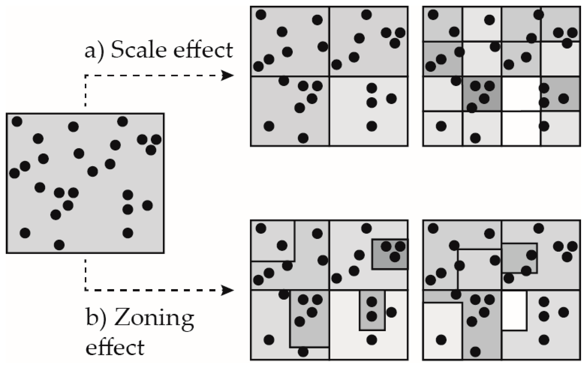
Generally, the definition of fixed spatial reference units is a trade-off between spatial details (heterogeneity) and statistical robustness of analyses that build upon these aggregates. Independently from the level of aggregation, derived patterns might be biased by the MAUP. The MAUP effect can be observed for regular (hex-, square-grid) and irregular (administrative units) reference units. It describes the effect of scale or level of spatial aggregation (
Figure 2a) and of zoning (
Figure 2b) [
34]. Although the MAUP effect can be quite large, it is hardly ever explicitly addressed in risk calculations for bicycle crashes. Frequently spatial reference units are defined by pragmatic reasons, such as the availability of statistical data. In the Geographical Information Systems for Transport (GIS-T) literatures [
35,
36], the MAUP is primarily dealt with in the context of transport modelling, where the delineation of traffic analysis zones (TAZ) raises the modifiable areal unit problem. Thomas [
37] and Abdel-Aty et al. [
28] are among the few studies that deal with the MAUP in the context of crash analysis and modelling. However, to our current knowledge, there is no study on bicycle risk calculation and mapping, which explicitly considers the MAUP.
1.3. Exposure Data
A major reason for why most risk calculations are based on highly aggregated statistics is the lack of adequate exposure data on a local scale [
13]. A recent Organization for Economic Co-operation and Development (OECD) [
38] report on this topic states, “The lack of exposure data is a real hindrance to understanding the current status of cycling safety and complicates the assessment of cycling policies” (p. 61). This statement is confirmed by virtually any study on bicycle risk calculations. International comparisons of safety performance tend to be biased by the heterogeneous quality of the exposure data. Tracing back the data sources of such studies (e.g., [
16,
20]) reveals extensive variabilities in spatial and temporal coverage. In addition to compiled statistics based on multiple statistic agencies, exposure variables are commonly derived from household travel surveys [
21], census data [
23,
39], and travel diaries [
14]. Data from these sources are samples that require model-based extrapolations in order to get full population data.
Alternative sources for exposure data are not exploited yet. To our current knowledge there are no bicycle risk analyses that rely on mobile phone, tracking or VGI data as exposure variables. However, studies reveal the potential of these data sources as proxies for collective mobility [
40,
41,
42].
Together with the severe underreporting of bicycle crashes in general [
43,
44,
45], the lack of adequate exposure data has, of course, far-reaching implications for the reliability and robustness of risk models. This holds especially true for models and analyses on the local scale, where hardly any of the existing approaches on the regional and national scale meet the demands in terms of accuracy and spatial resolution.
2. Method
In order to provide reliable bicycle crash risk analyses on the local scale level, while considering the issues discussed in the previous section, we followed an iterative workflow which helps to identify adequate reference units and tests the robustness of crash rates for various unit sizes. We demonstrate the applicability of the workflow in a case study from Salzburg (Austria).
2.1. Study Site
Located in the northern Alps of Austria, the city of Salzburg, capital of the homonymous province, has roughly 150,000 inhabitants. Another 150,000 people live in the larger agglomeration, within a radius of 15 km from the city center. Thus, the city has a catchment of approximately 300,000 inhabitants within cycling-distance.
The road network of the study area (city of Salzburg), which is legally relevant for bicycle traffic has a total length of 1045 km. Within the city a total of 320 road km are equipped with some kind of bicycle infrastructure, ranging from separated bicycle ways to opened one-way roads with painted on-road cycle lanes. According to the latest available figures, Salzburg has a 20% share of the bicycle in the total modal split [
46]. The reasons for the popularity of the bicycle as utilitarian mode of transport are manifold. The flat topography, high-quality bicycle infrastructure along main corridors, short distances and a good accessibility of central facilities are commonly regarded as major attractors.
2.2. Crash Data
The crash data used for this study consists of over 3000 police crash reports and covers a time period of 10 years (2002–2011). The federal bureau of statistics (Statistik Austria) is responsible for crash data collection in Austria and publishes an annual national road crash report. Usually, the collected and processed police reports are reported back to the respective authorities. In the case of the city of Salzburg, the department of urban planning and transport maintains the crash database for all road incidents within the city. This authoritative dataset is exclusively fed by police reports. Hence, hospital records [
47], insurance claims [
48], crowdsourced information [
49], or other alternative data sources are not included.
No estimations for the underreporting rate of bicycle crashes exist for the city of Salzburg. However, indications for the dimension of the problem are available in the literature. Watson et al. [
44] showed that two thirds of bicycle crashes that were reflected in hospital data could not be linked to police reports in Queensland (Australia). De Geus et al. [
14] estimate a fraction of only 7% of all minor crashes are being reported to the police in Belgium. Similar underreporting rates are presented by Janstrup et al. [
50] for the Danish province of Funen. Although these rates cannot be directly transferred to the city of Salzburg, we must be aware that the data used in this study might only cover a maximum of one third of all crashes. However, it can be assumed that regions with an increased crash risk can be identified with the proposed workflow, because crashes with severe injuries and high material damage tend to be captured more probably by police reports.
For the purpose of this study crash reports, with at least one involved bicyclist and valid location information, were extracted from the database. A total of 3045 geolocated crash reports between January 2002 and December 2011 met both criteria and were thus considered for further analysis; 51 crash reports suffered from invalid location information. In the present case, only location information for the risk calculation was relevant. Thus, associated data about the involved parties, liabilities and crash details were not considered.
2.3. Exposure Variable
As demonstrated in
Section 1.3, commonly employed exposure data is not suitable for the mapping of local risk patterns. Thus, we used the results from a spatial simulation of bicycle flows as the exposure variable for this study. For details concerning the agent-based simulation model itself we refer to Wallentin and Loidl [
51].
The agent-based model (ABM) simulated the total number of traverses per segment for one day (6 June 2014). Segments are the spatial increment of the digital representation of the road network. In our case, the road network was modelled as an undirected graph, where nodes correspond with junctions and edges with segments. In accordance with Yiannakoulias et al. [
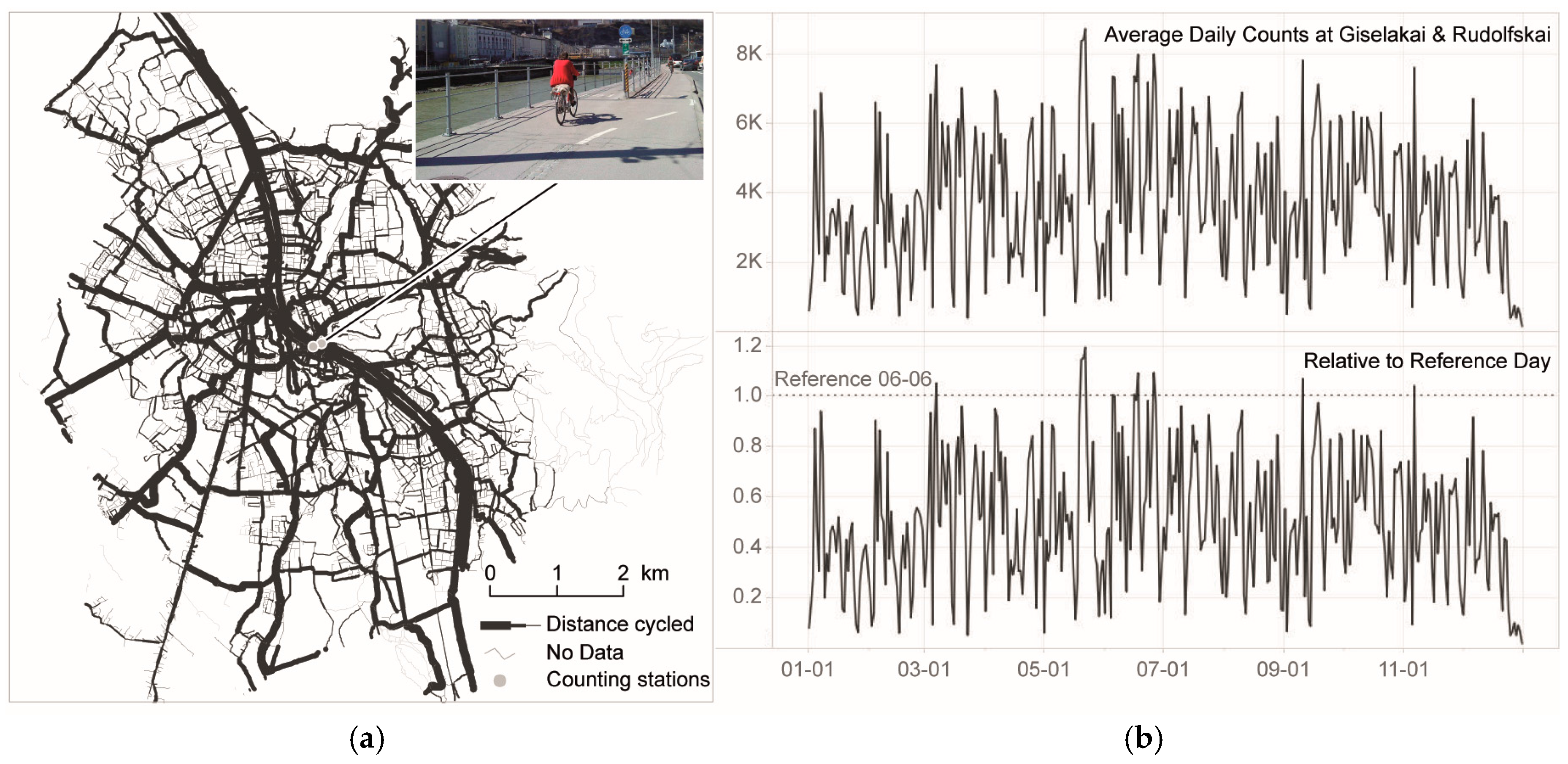
23] we did not employ the number of traverses (or trips) as the exposure variable, but the total distance travelled. Thus, the number of traverses was multiplied with the segment length. Based on the simulation of a single day and counting data for the whole year 2014 the flows (total distance travelled) were extrapolated accordingly (
Figure 3). This extrapolation exhibits a certain degree of generalization, as the implicit assumption is that variabilities over time are evenly distributed over space.
The crash data covered the years from 2002 to 2011. Unfortunately no counting data was available for the entire time period. Thus, we multiplied the simulated annual flow by 10, disregarding the change of bicycle traffic over time. For the current state of research this degree of generalization was tolerated, since alternative exposure variables are by far less suitable for the purpose of local risk mapping and the focus of this study was on spatial patterns.
2.4. Conceptual Workflow
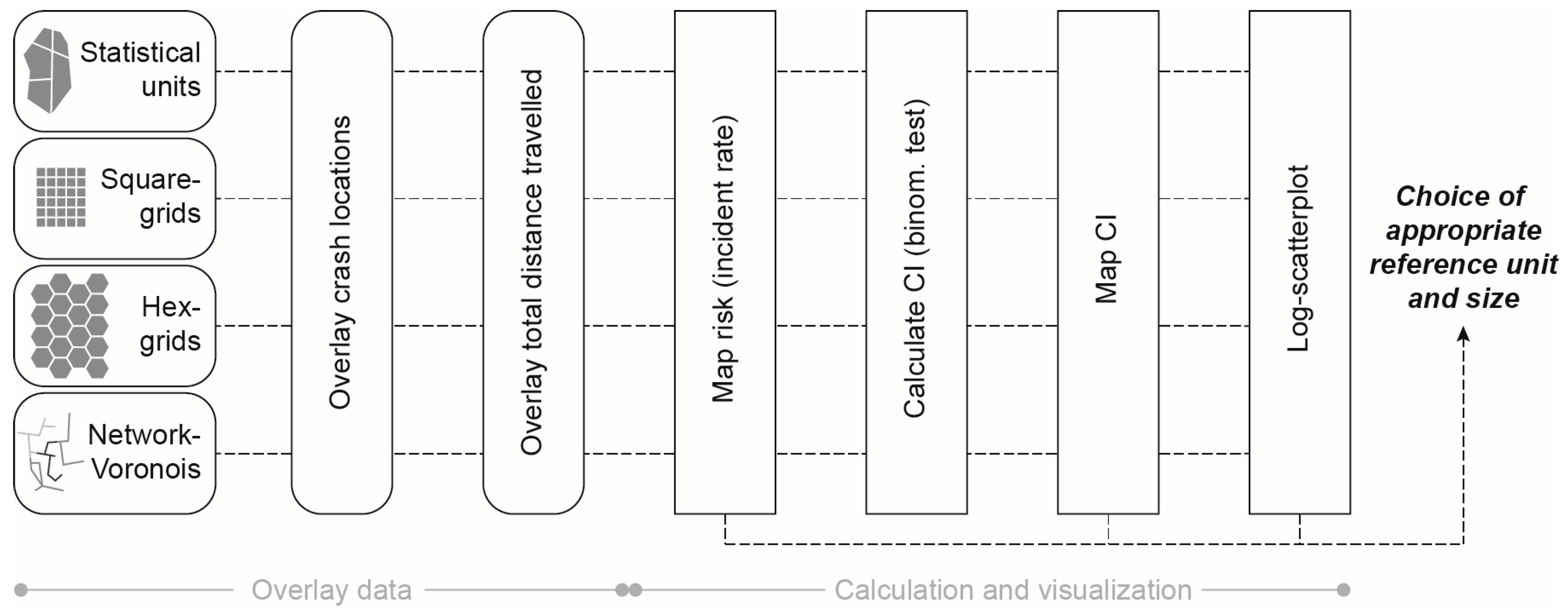
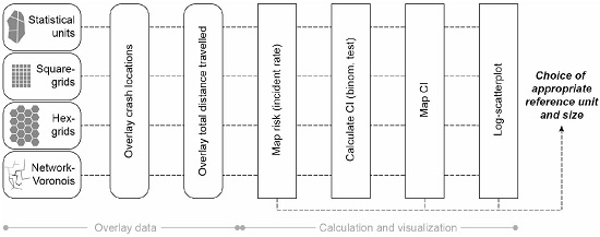
The aim of this study was to map bicycle risk patterns on the local scale, in order to account for spatial variabilities adequately (see
Figure 4 for the overall workflow). Although the geolocated crash data and the simulated flow would allow for risk calculations on the level of road segments, the data was aggregated for the sake of statistical robustness. Consequently, the decision on the most suitable spatial reference unit (level of aggregation) was a trade-off between the amount of spatial heterogeneity and the size of the confidence interval of the risk calculation. Additionally, the MAUP was to be considered.
In order to test the type of reference unit and the effect of the unit size, irregular and regular reference units were defined. Additionally, network-based reference units were generated (for the algorithm for the delineation of network-based units we refer to Loidl et al. [
30]).
Each reference unit was overlaid with the geolocated crash reports and the total distance travelled. The high standard deviations for the number of crashes per reference unit in
Table 1 indicate that crash locations and bicycle flows are unevenly distributed over space, what is in line with a previous study [
30,
31]. For the present study the following spatial reference units were tested.
Based on the number of crashes and the simulated total distance travelled, the risk was calculated for each reference unit. These crash rates were only calculated for reference units where both crash data and simulated flows were available. When these risk calculations had been mapped, spatial patterns emerged.
The problem with bicycle crashes is that they are rare events and it is decisive for any interpretation to identify random occurrences. Thus, a measure is required that determines the robustness of derived risk calculations (crash rate). In order to do so, a 95% confidence interval was calculated for each reference unit applying an exact binomial test [
52] as implemented in the open source software package “R” (
https://www.r-project.org/). The size of the confidence interval indicates the robustness of risk calculations and helps to interpret crash rates. The larger the confidence interval, the lower is the statistical robustness, and the higher is the chance that the calculated risk is the product of random processes or an artefact. In order to provide information about the quality of calculated crash rates, the risk map was complemented with mapped confidence interval sizes.
With regard to the trade-off between spatial heterogeneity and statistical robustness we made use of a scatterplot with logarithmically scaled axes. With this, we were able to plot the calculated risk, the number of accidents and the size of the confidence interval. Based on this scatterplot, reference units with a maximum visual compactness could be identified. Together with the mapped crash rates and confidence intervals, the scatterplot served as a decision basis for the choice of appropriate reference units. MAUP effects could be identified through the link of map series and the scatterplot.
3. Results
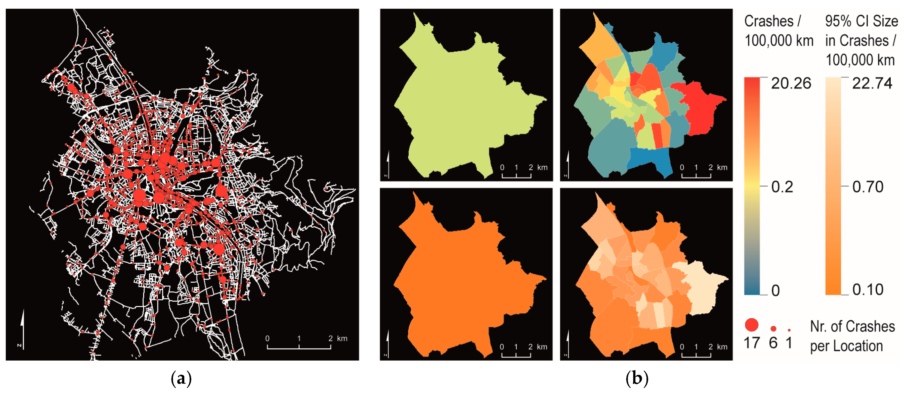
As it becomes obvious in
Figure 5, crash locations are not evenly distributed over space, but clustered. This spatial heterogeneity cannot be captured when the city is investigated as a whole. On average 1.43 crashes per 100,000 km cycled (95% Confidence Interval (CI) [1.38…1.48]) occurred during the 10 years of investigation. Aggregating the data to census districts reveals distinct patterns of risk distribution. Interestingly the frequency of crash occurrences does not directly correspond with the crash rate. The highest crash rates emerge north of the city center and in the very east-most region. However, the high risk in the eastern district can be identified as an artifact by the mapped confidence interval. For this area a very low flow was simulated because the model concentrated on utilitarian trips. The statistical district in the east covers a mountainous area with lots of leisure cycling. Consequently, the number of crashes is disproportionately high in relation to the simulated total distance traveled. In contrast to this particularity, the comparable high risk in the districts around the city center is statistically more robust and should, thus, be subject to further analyses.
Although natural barriers (river, railway, etc.) and population density are commonly considered in the definition of census districts, they are still hard to compare. Additionally, phenomena that are not constituted by a static population but by dynamic elements (e.g., bicycle traffic flows generated by commuters) are not fully captured by census districts. In our case major corridors with high volumes of in- and out-flux are relevant. This becomes evident when considering the statistical district in the very north-most region. It covers a large area and the calculated crash rate is relatively high. In fact, there is an important bicycle corridor, connecting the city center with the adjacent municipality along a primary road. The crashes are concentrated along this road, while there are hardly any other crash locations in the whole district. Thus, the spatial heterogeneity within this district is high and calls for further disaggregation.
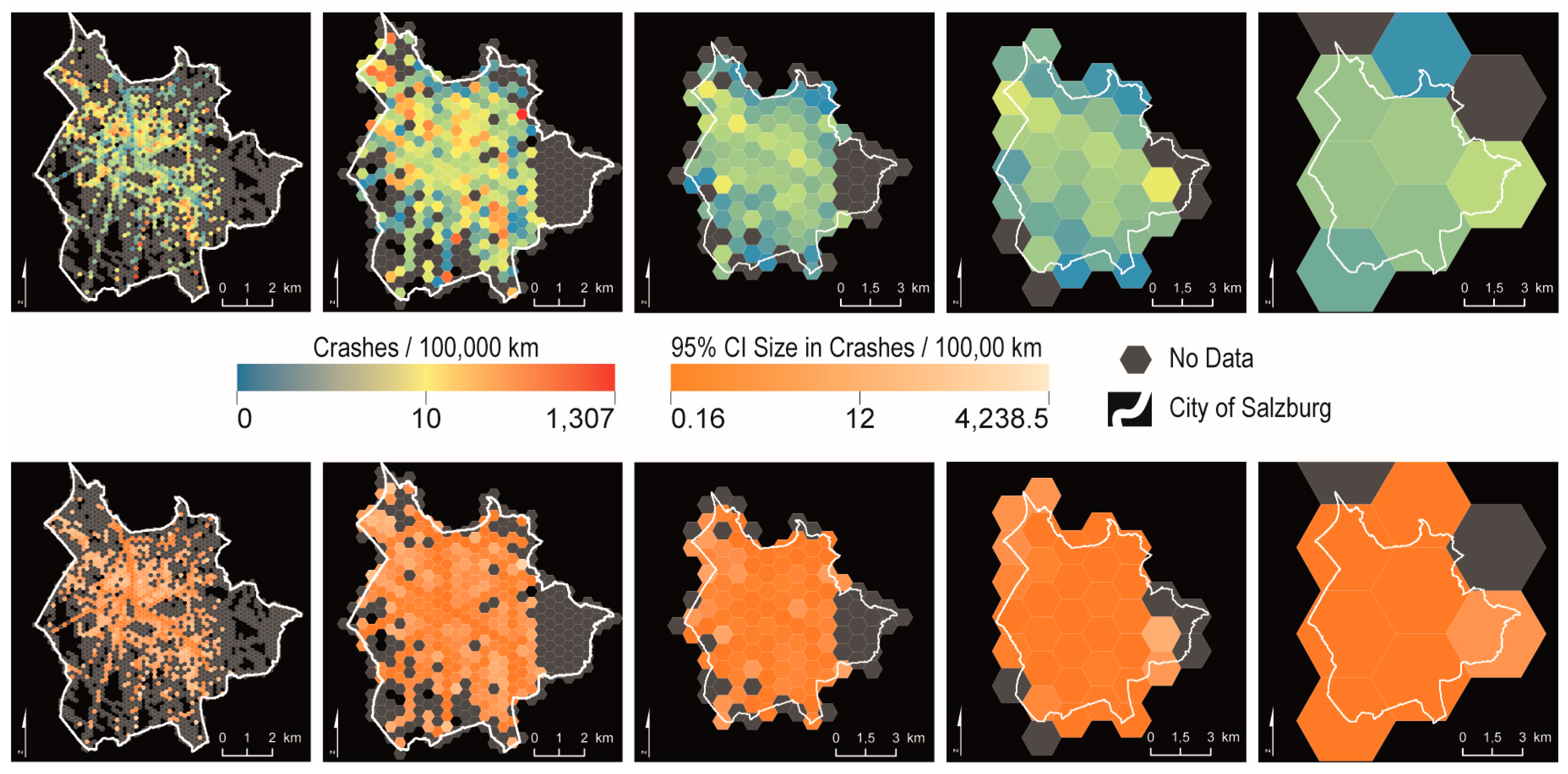
Different to census districts, regular reference units are equal in size. On the one hand this helps in the interpretation of results because there is no need to control for the area. On the other hand, underlying structures are not considered in the definition of the reference units and, thus, the MAUP becomes an eminent issue. In the present case regular reference units are primarily used to calculate crash rates for various levels of aggregation.
Hex grids are the most compact units that can cover the entire planar space without gaps. This explains their popularity in domains that deal with continuous phenomena, such as ecology [
53]. Apart from the type of the reference unit, the size strongly influences the patterns that emerge.
Figure 6 maps the risk calculations for five different levels of aggregation. The smaller the reference units, the better local particularities are mapped. However, as the reference units with the two lower levels of aggregation cover only very small areas each, they are prone to extreme outliers (as the range of values in the legend indicates) and artifacts. These values can only be interpreted in conjunction with the mapped confidence intervals.
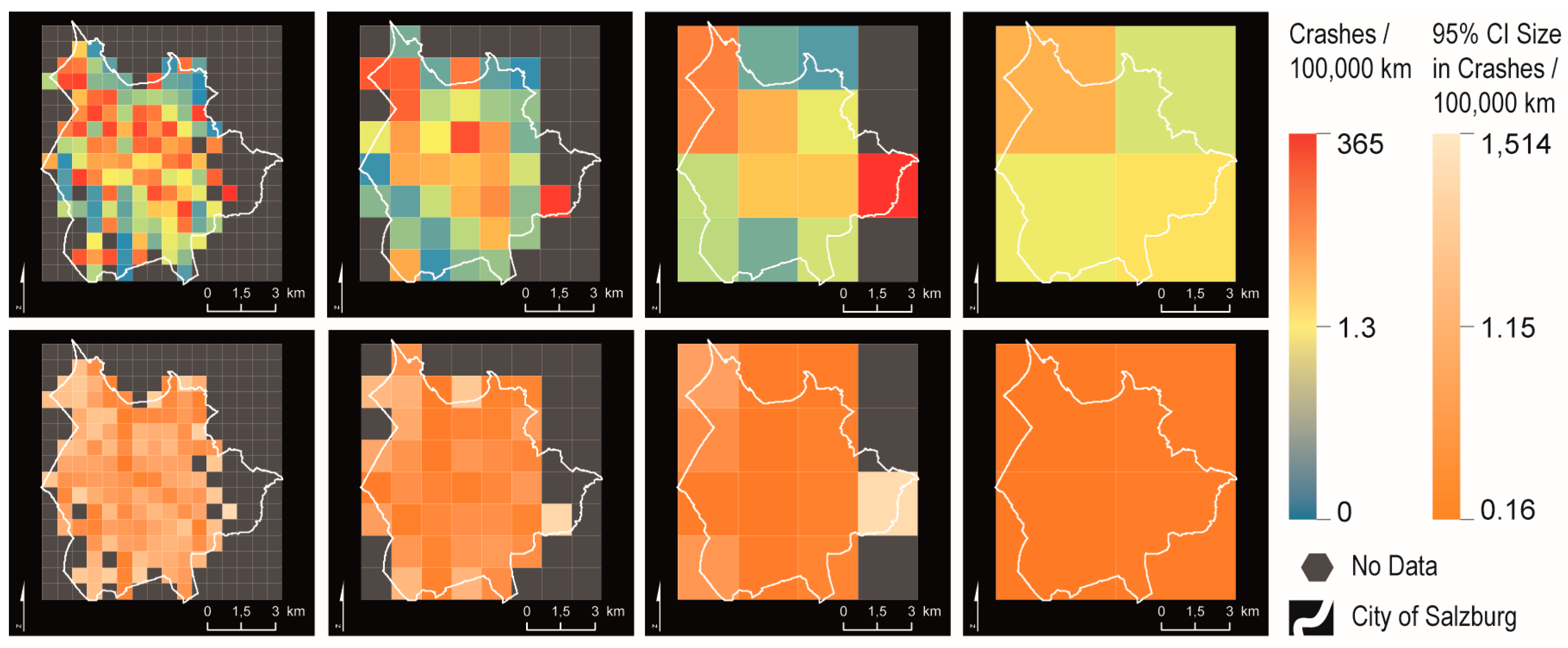
Mapping the risk calculations based on square grids reveals patterns that are in some parts different from the hex grid (
Figure 7). This is due to the shape and to the respective size. Comparing the two maps in the center nicely demonstrates the MAUP (scale effect). Whereas the map with the higher level of aggregation shows a rather low risk level in the north, the pattern is different at a lower level of aggregation. However, again, the mapped confidence interval is decisive for judging on the quality (statistical robustness) of this local particularity. The square grid maps with different levels of aggregation (
Figure 7) demonstrate the spatial heterogeneity within aggregated units. Decomposing the reference unit in the northwest of the map with the highest level of aggregation reveals the variability within this aggregate. In the present case it becomes obvious that the areas with a high crash rate are concentrated along a corridor.
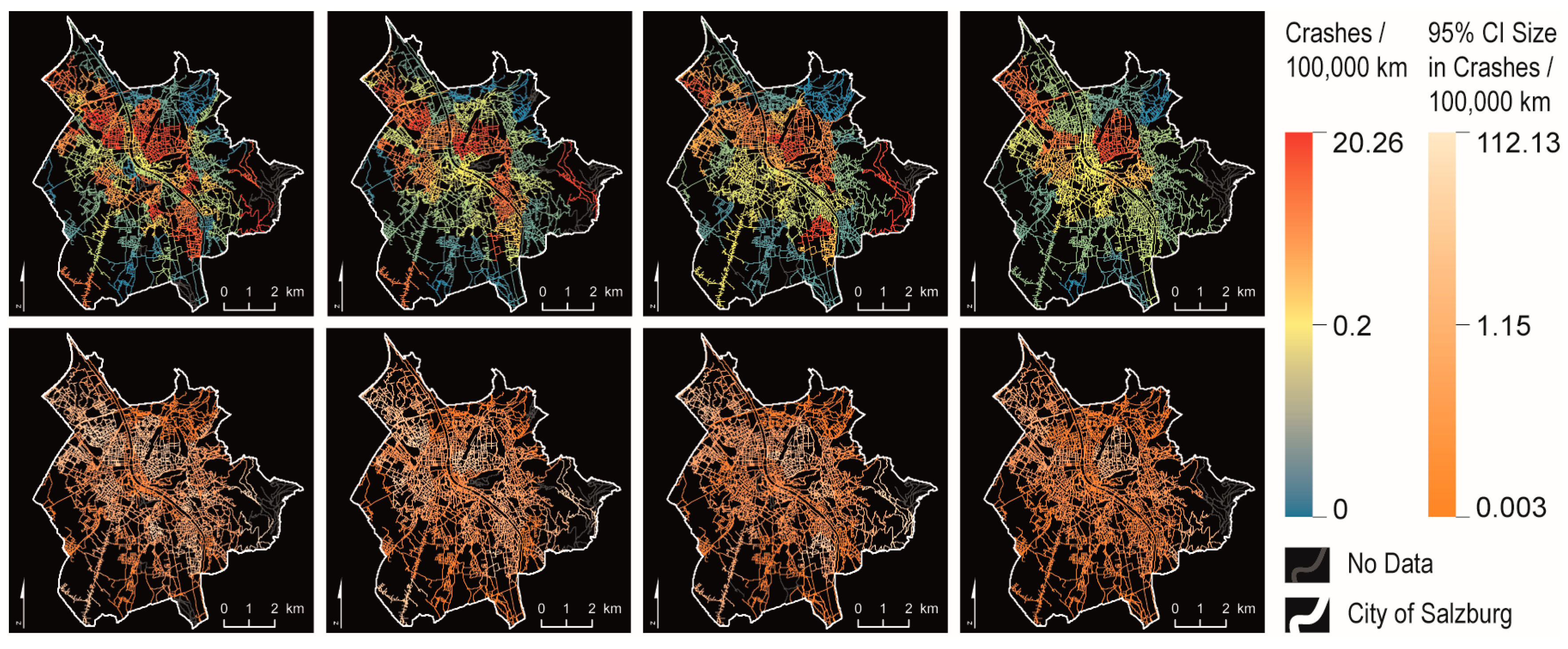
As argued before, bicycle crashes are network-bound incidents. Thus, planar reference units neglect this characteristic to a certain degree, which can lead to biased analysis results. Take for example two locations with a significantly high number of crashes. In reality these two locations are disconnected (e.g., by a river) but close to each other, when only the Euclidean distance is considered. It might happen that these two locations are aggregated to the same spatial reference unit, indicating an area with high risk, although there is no relation in reality. Considering this argument, we also tested different network-based reference units (for details refer to [
30,
54]).
Figure 8 shows the effect of network-based reference units on the emerging patterns. Depending on the level of aggregation, regions in the network with a high crash rate become obvious that tend to be hidden in planar reference units. Similar to
Figure 7, the MAUP effect can also be observed in this case (see the reference units with high risk in the east).
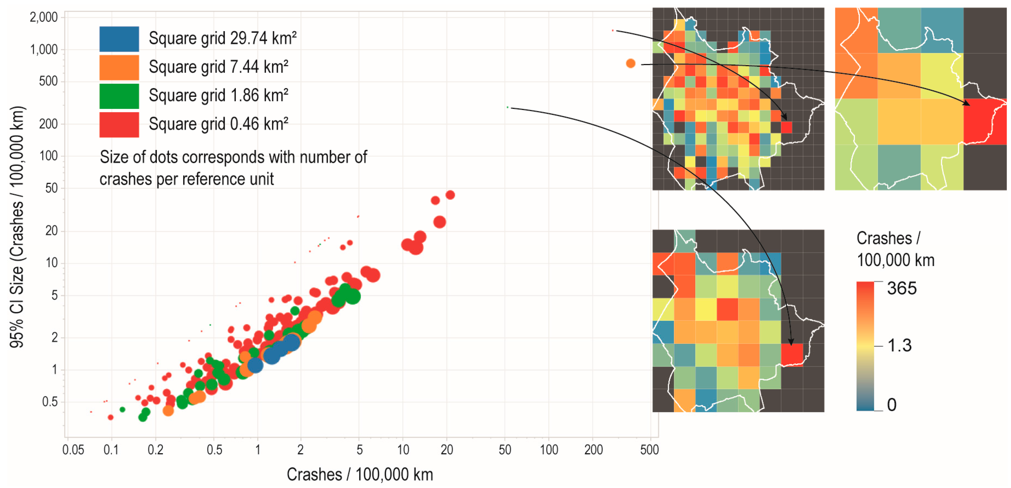
Whereas spatial patterns become obvious from maps, the statistical distribution of crash rates and confidence intervals remains hidden. Therefore, we link the maps with a scatterplot for each type of reference unit.
Figure 9 shows the result for the square grid reference units.
The scatterplot, together with the maps help to identify outliers and to decide on an optimal level of aggregation for a given purpose. The visual compactness of the points in the scatterplot indicates the similarity of the reference units. Generally there is a direct relation between the size of the reference units (generalization through aggregation) and the visual compactness in scatterplot. However, in the case illustrated in
Figure 9, the higher level of aggregation (orange dots) is less compact (higher range of values on both axes) than the finer grid (green dots). In this case one might conclude that the finer grid is to be preferred, as it better represents the spatial and the statistical distribution.
4. Discussion
The results confirm the assumption of a high degree of spatial heterogeneity within highly aggregated reference units. However, the MAUP and random crash occurrences can bias the emerging examples significantly. In the following we want to discuss this trade-off referring to selected results.
4.1. Spatial Heterogeneity and Local Particularities
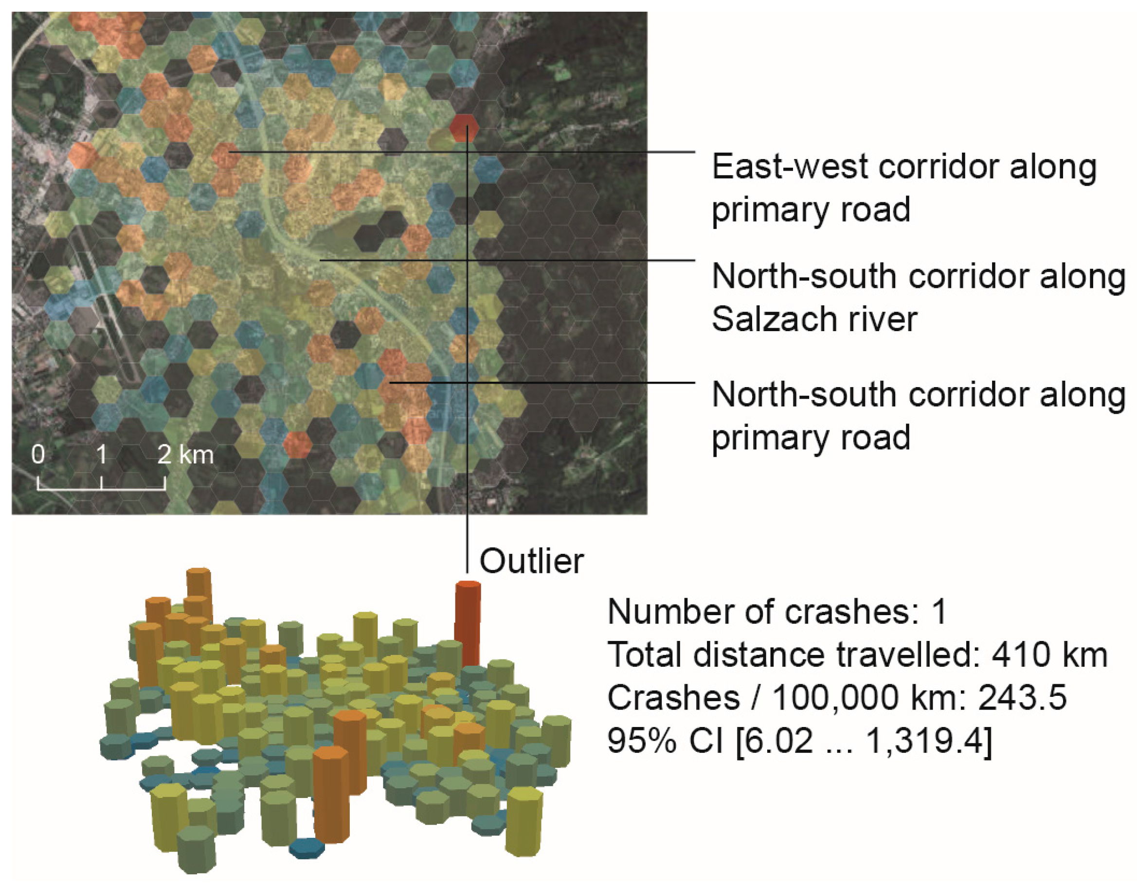
Figure 10 demonstrates the additional insight that is gained from risk mapping on a local scale. It reveals distinct spatial patterns of risk, which are neither captured in the analysis of absolute numbers of crashes [
30] nor in aggregated statistics.
By far the most bicycle traffic occurs along the Salzach River in a north-south direction. From the analysis on the local scale it can be concluded that although most crashes occur along this corridor (
Figure 5), the risk is comparably low. The situation is quite different in the north and in the south of the city centre (the corridors are indicated in
Figure 10). Here, the number of crashes is high in relation to the simulated volume. In both areas bicycle infrastructure (mixed cycle-/pedestrian way and on-road cycle lanes) runs along primary roads with a very high traffic load. Thus, dangerous situations inevitably occur at intersections where connector roads cross the bicycle infrastructure. In sum, it can be concluded from this particular example, but also from the maps in
Figure 5,
Figure 6,
Figure 7 and
Figure 8 that high risk is not primarily a function of bicycle traffic volume (although the bias in the crash reports, namely the overrepresentation of bicycle-car collisions, need to be considered!), but more of the combination of different modes and infrastructure types.
Generally, the mapping of crash risks on the local scale facilitates additional insights and contributes to a better understanding of spatial variabilities of risk patterns. However, outliers might distort these emerging patterns. From the example, mapped in
Figure 10, one might conclude that an extremely dangerous hot spot exists in the northeast of the study area. In fact, the high risk is due to the small population (total distance travelled). Therefore the confidence interval is very large; the single crash recorded in this reference unit can be regarded as random. In accordance with the maps in
Figure 5,
Figure 6,
Figure 7 and
Figure 8 the necessity for a statistical measure to judge on the robustness of the results becomes obvious. For independent events, which occur at rare intervals, the confidence interval determined by an exact binomial test [
52] is proven to be an adequate measure, independent from the type of reference unit. Providing a measure for the robustness of calculated crash rates is especially important for small reference units and for areas at the periphery of the area under investigation, since the probability of artefacts is higher here than in more central areas.
4.2. Scaling and Zoning Effects (Modifiable Areal Unit Problem, MAUP)
As conceptually discussed in
Section 1.1, the MAUP affects the emerging patterns on the risk maps. Independently from the large confidence interval (
Figure 7) for the reference unit mapped in
Figure 11, the map series illustrates both the scaling and zoning effect.
The mapped region is located at the periphery of the study area. This is why for some reference units no flows are simulated (in grey). Depending on the level of aggregation and the size of the reference unit respectively, the risk that is communicated by the map tends to be spatially overestimated. In fact, only 1/16 of the largest grid data is available. Therefore, the level of aggregation (scaling) heavily influences the conclusion that might be drawn from the emerging spatial pattern.
In addition to the scaling effect,
Figure 11 also illustrates the zoning effect. The single crash location in the highlighted reference unit is located close to the boundary. Grid cells are, of course, an arbitrary decomposition of a continuous space. Shifting the whole grid, for example in south direction, would impact the mapped result in this case significantly. The risk for the respective cells would be 0 for all levels of aggregation.
4.3. Results and Limitations of the Proposed Workflow
Producing map series with various types of reference units and different levels of spatial aggregation makes the influence of these parameters on the emerging spatial patterns visible. From the hex grid maps continuous corridors can be derived best and MAUP effects are minor. However, the result for the lowest level of aggregation exhibits a large degree of uncertainty. For the maps based on square grids we showed the effect of the reference unit’s size. Additionally, MAUP effects tend to occur often, due to the less compact shape compared to hex grids. The network-based reference units are valuable and provide additional insights, as the connectivity of locations is considered. Although the algorithm for generating these units aims to produce units of equal size, they are hard to compare. Hence MAUP effects impact the emerging patterns considerably. In sum, the case study demonstrates that, for a final decision on most optimal reference units, information on the robustness of the results and an overview of alternatives is necessary. Additionally, the purpose of the map (e.g., city overview versus in-depth investigation of a specific corridor) ultimately decides the type and size of the spatial reference units.
As our approach heavily relies on models, the results exhibit a certain degree of generalization. This holds especially true for the agent-based simulation model and the extrapolation of the total distance travelled for the entire period from 2002 to 2011. However, there are no studies yet, which draw exposure data from full population surveys (see e.g., [
13,
14,
21,
23]).
In addition to the quality of the exposure variable the crash data directly impacts the emerging patterns. We assume that more complete crash data would lead to slightly different results. For example, along the Salzach River the calculated risk is comparable low (
Figure 10). This might be due to the severe underreporting of single-bike-crashes (SBC, [
55]) and bicycle-bicycle collisions. Dealing with risk, not only de facto crashes, but also near misses are considered as relevant. Here additional data sources, such as the BikeMaps.org project [
49], would complement conventional data sources.
5. Conclusions
We have shown that mapping bicycle risk patterns on the local scale reveals relevant information, which aggregated approaches would not have been able to uncover. To our current knowledge this is the first study, which calculates crash rates on the local scale. The lack of adequate exposure data on this scale level has been the restricting factor up to recently. This can be overcome through the utilization of simulated bicycle flows as exposure variable.
With the calculation of risk on the very local scale, the spatial heterogeneity is directly accounted for. On the other hand the issue of statistical robustness and the MAUP effect become eminent. In order to assess the quality of calculated crash rates, we calculated the 95% confidence interval for each spatial reference unit. These two information layers can be visually linked (as in
Figure 5,
Figure 6,
Figure 7 and
Figure 8), overlaid (as in
Figure 10, where the units are extruded proportionally to the size of the confidence interval) or plotted in a scatterplot (
Figure 9). This way, we were able to identify outliers and artifacts and to facilitate valid interpretations of emerging spatial patterns. With regard to the MAUP effect we provided map series with different types of reference units (shape) and levels of spatial aggregation (size). This way we were able to make MAUP effects for bicycle risk patterns explicit. Although the results presented in this paper are specific for the city of Salzburg, the conceptual workflow is transferable to any city as long as geolocated crash reports and exposure data are available.
The proposed workflow for mapping bicycle risk patterns on the local scale extends existing approaches in spatial risk analysis. In addition to methodological improvements that stem directly from the limitations discussed in the previous section, further research should focus on the following aspects:
Temporal dynamics: it is generally known from literature that crash occurrences depend on a number of influential variables. Among the most relevant is time. Future risk mappings on the local scale should consider temporal dynamics, such as weekday-weekend patterns or seasonality [
30]. In conjunction with the spatial dimension this might help to launch effective and adaptable interventions for increased bicycle safety.
Subgroups: existing studies suggest different behavior depending on gender, age or trip purpose [
17,
18,
19]. It is to be investigated to which degree these differences are reflected in distinct spatial patterns.
Crash types: in this study all crashes were considered equally. In order to allow for an adequate design and a prioritization of interventions, areas of high risk must be identified, considering the crash type and severity.
Explanatory analyses: once the risk is estimated for particular areas, it is of greatest interest to reveal causal factors, which contribute to the risk. Current studies (for instance [
47,
56]) consider the spatial configuration mostly implicitly or neglect it at all. However, geographical information systems (GIS) provide a platform to relate multiple perspectives on the road space [
57]. Consequently, findings from studies on risk patterns on the local scale level can be related to information on infrastructure, crowd-sourced user feedback, or results from traffic flow models in further analyses.

