Abstract
In hyperspectral image (HSI) classification, convolutional neural networks (CNNs) have been widely employed and achieved promising performance. However, CNN-based methods face difficulties in achieving both accurate and efficient HSI classification due to their limited receptive fields and deep architectures. To alleviate these limitations, we propose an effective HSI classification network based on multi-head self-attention and spectral-coordinate attention (MSSCA). Specifically, we first reduce the redundant spectral information of HSI by using a point-wise convolution network (PCN) to enhance discriminability and robustness of the network. Then, we capture long-range dependencies among HSI pixels by introducing a modified multi-head self-attention (M-MHSA) model, which applies a down-sampling operation to alleviate the computing burden caused by the dot-product operation of MHSA. Furthermore, to enhance the performance of the proposed method, we introduce a lightweight spectral-coordinate attention fusion module. This module combines spectral attention (SA) and coordinate attention (CA) to enable the network to better weight the importance of useful bands and more accurately localize target objects. Importantly, our method achieves these improvements without increasing the complexity or computational cost of the network. To demonstrate the effectiveness of our proposed method, experiments were conducted on three classic HSI datasets: Indian Pines (IP), Pavia University (PU), and Salinas. The results show that our proposed method is highly competitive in terms of both efficiency and accuracy when compared to existing methods.
1. Introduction
Hyperspectral image (HSI) classification is a hot topic in the field of remote sensing. HSIs, captured by airborne visible/infrared imaging spectrometer (AVIRIS), provide rich spectral and spatial information that is highly valuable for the fine segmentation and identification of ground objects. Therefore, HSIs have been widely applied in various fields such as geological exploration, military investigation, environmental monitoring, and precision agriculture [1,2,3,4].
In the past decades, traditional feature extraction methods for HSI classification, such as k-nearest neighbor [5], random forest [6], Markov random fields [7], and support vector machines (SVM) [8], have been widely used. However, these methods require manual labeling and expert experience, which make them expensive and limited in their ability to extract high-level features. Additionally, HSIs with redundant information also pose challenges for classifiers.
Deep learning methods have received significant attention for their ability to automatically learn robust features from training samples. These methods have been successfully applied to HSI classification, including stacked autoencoder (SAE) [9], recurrent neural network (RNN) [10], deep belief network (DBN) [11], CNNs [12,13,14], and others. These approaches have achieved remarkable results when compared to traditional methods. Chen et al. [15] first introduced deep learning into hyperspectral data and used SAE to obtain spectral and spatial features, respectively, to achieve classification. Later, Hu et al. [16] used five 1×1 convolution layers to capture spectral information for HSI classification but ignored the importance of spatial information. Ying et al. [17] proposed a 3-D convolutional neural network to extract spectral-spatial features of 3-D hyperspectral images to achieve accurate classification of HSI. Yang et al. [18] proposed a two-channel deep convolutional neural network model (TCCNN) to extract joint spectral-spatial features of HSIs and two branches were used to extract spectral and spatial features, respectively. Chen et al. [19] added 3-D convolution to extract spectral-spatial features of HSI based on TCCNN, and the results show that the method is effective. However, 3-D CNN will cause excessive training parameters and high calculation costs. As neural networks become deeper, the extracted features become more abstract and robust. However, the limited number of training samples can lead to overfitting. To address this problem, Zhong et al. [20] and Wang et al. [21] used residual connections [22] and dense connections [23], respectively, to enhance the robustness of the network and avoid overfitting. Due to the ability to perform convolutions on arbitrary graph structures, graph convolutional networks (GCNs) have been applied to HSI. Qin et al. [24] proposed a semi-supervised GCN method, which can flexibly encode irregular non-Euclidean data and effectively express the relationship between each node. However, it requires a large amount of computing cost to construct an adaptive graph structure.
Attention mechanisms [25] have gained attention in the field of vision for their ability to focus on important information and disregard redundant information. The transformer model uses a multi-head self-attention (MHSA) module to capture long-range dependencies in input sequences. Song et al. [26] proposed a hierarchical transformer network that uses MHSA to better extract spectral-spatial information. However, the computational cost of MHSA is high due to the excessive dot-product operations involved. T et al. [27] combined the Squeeze-and-Excitation (SE) Network, known for its effectiveness in channel attention, with CNN for HSI classification, effectively utilizing spectral information. Similarly, Sun et al. [28] proposed a spectral-spatial attention mechanism, adding spectral and spatial attention to each traditional convolution, enabling a higher focus on useful information and improving the classification accuracy. Li et al. [29] proposed a double-branch dual-attention network (DBDA) to capture spectral and spatial features separately, to achieve refinement and optimization of the extracted features. And the coordinate attention network (CA) [30] was proposed to address the high computational cost and complexity of the attention mechanism. It retains spatial coordinate position information and captures global information of image pixels.
Although the above methods have already achieved promising results, they are still facing some problems. (1) The classification performance of CNN-based methods for HSI classification is limited by the size of the convolutional kernels, and it is difficult to capture long-range dependencies between pixels in HSI. (2) HSI typically contains hundreds of continuous spectral bands, but not all bands contribute equally to classification accuracy. The invalid bands not only increase computational cost but also degrade classification performance. (3) Existing methods for HSI classification have complex network architectures, which can lead to inefficient classification results.
Inspired by the attention mechanism, this paper proposes an effective HSI classification network based on MHSA and spectral-coordinate attention. The proposed method first uses a point-wise convolution network (PCN) to remove redundant spectral band information and provide more discriminative features. Then, an M-MHSA module is introduced, which down-samples the k and v projections to a low-dimensional embedding to alleviate the computing burden caused by dot-product operations in MHSA. The method also assigns weights based on pixel correlation to capture long-range dependencies among the HSI pixels, addressing the limitations of CNNs having a small receptive field. Furthermore, a lightweight spectral-coordinate attention fusion network is proposed. On the one hand, spectral attention is used to model the importance of each spectral feature and suppress invalid channels. On the other hand, the coordinate attention network is used to aggregate features along two spatial directions, which addresses the limitation of MHSA ignoring inherent position information and strengthens the connection between channels. Finally, we conducted experiments on three classical datasets, Indian Pines (IP), Pavia University (PU), and Salinas. The experimental results demonstrate that our proposed method is highly competitive among existing HSI classification methods.
2. Proposed Methods
The goal of HSI classification is to assign a specific label to each pixel in order to represent a particular category. In this paper, we propose an effective network based on multi-head self-attention and spectral-coordinate attention (MSSCA). The overall architecture of the proposed network is depicted in Figure 1.
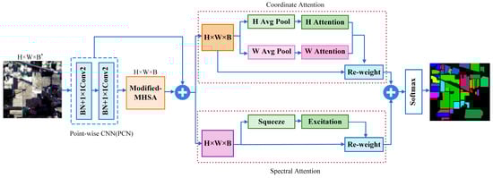
Figure 1.
The overall network architecture of the proposed MSSCA.
2.1. Point-Wise Convolution Network (PCN)
HSIs often contain redundant bands, which not only increase computational complexity but also negatively impact classification accuracy. To reduce the redundant information and provide more discriminant features for subsequent networks, we propose the PCN to process the band information of the HSI. Specifically, let as the HSI input, and the PCN is composed of two 1×1 convolutional layers. Using this network, the output feature map can be expressed as:
where represents the output representation of the feature map of the l-th spectral convolution layer, represents the value of the j-th output feature channel in the l-th layer, denotes the input feature mapping of the (l-1)-th convolution layer after batch normalization, and represent the j-th convolutional kernel with the size of 1 × 1 and the bias in the l-th layer, respectively, and is the activation function. The resulting PCN output is then fed as input to subsequent networks, providing robust and discriminative initial spectral characteristics for these networks.
2.2. Modified Multi-Head Self-Attention (M-MHSA)
The transformer has gained significant attention in computer vision due to its successful applications. Specifically, the self-attention mechanism, which is a key component of the transformer, is capable of capturing long-range dependencies, making it an attractive technique. In this paper, an M-MHSA network is introduced, where K and V are projected to a low-dimensional embedding using a lightweight down-sampling. This operation reduces the computing burden caused by performing attention calculations on all pixels, while simultaneously enriches feature subspace’s diversity by independent attention heads. Moreover, it assigns weights based on the inter-pixel correlations, allowing for the extraction of global feature dependency and overcoming the limitation of the small receptive field of a traditional CNN. The network architecture of M-MHSA is shown in Figure 2.
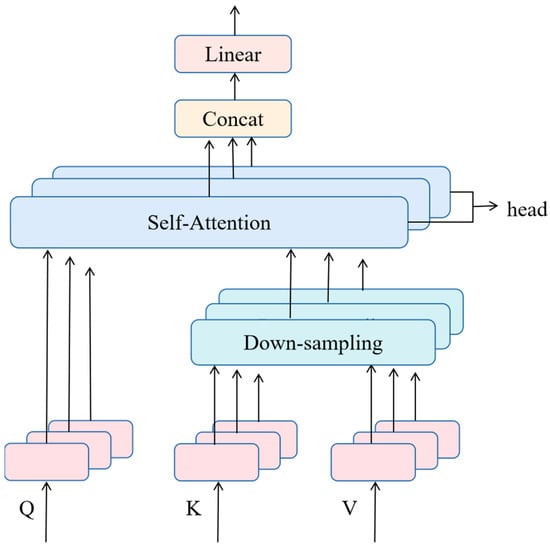
Figure 2.
The architecture of the modified multi-head self-attention.
Hyperspectral pixels can be viewed as a sequence of vectors . Each vector is multiplied by three weight matrices to obtain Query (Q), Key (K), and Value (V). The linear transformation for this process can be expressed as follows:
where , , and represent the transformation matrix of Q, K, and V, respectively.
The attention weight calculation can be expressed as:
where dk represents the dimension of Q and K.
To focus on different parts of the feature representation and extract richer long-range dependencies, Q, K, and V are divided into h submatrix as follows:
where h represents the number of heads.
The i-th head can be expressed as:
where .
Multiple independent heads are spliced together to form MHSA, so MHSA can be expressed as:
where indicates the output projection matrix.
To reduce the computational burden caused by dot product of Q and K, we propose to perform down-sampling on K and V after obtaining them, while preserving important information. Specifically, we reduce the spatial dimensions of K and V from (H × W) to (16 × 16), which in each head. This not only reduces the computational cost but also enables the network to capture long-range dependencies of the input image pixels. The modified MHSA can be expressed as:
where function represents a down-sampling operation.
2.3. Spectral-Coordinate Attention Fusion Network (SCA)
HSIs typically contain hundreds of bands, but many of them contribute little to the HSI classification and thus lead to poor classification performance. In this work, we perform spectral attention and coordinate attention for better utilization of the discriminative spectral and spatial features present in HSIs. Finally, we perform feature fusion to further enhance the HSI classification performance.
2.3.1. Spectral Attention
As shown in Figure 3, we incorporate the SE-Net architecture to recalibrate the spectral features in the HSI to strengthen the connections between spectral bands. This helps the network focus on valuable spectral channel information while suppressing irrelevant or invalid characteristic channel information.
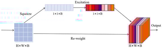
Figure 3.
The architecture of spectral attention module.
Let represents the input of SE network and represents b-th channel of feature mapping. By using a squeeze operation Fsq, the input feature map can be compressed along the spatial dimension, reducing two-dimensional features to one-dimensional data. This is achieved through global average pooling. generated by squeeze can be expressed as follows:
This operation is equivalent to indicating the value distribution of b feature maps. represents the element value of the b-th feature map at position (i, j).
The two fully connected layer networks are utilized to automatically learn the interdependency between different channels, with the importance of each channel determined by learned weight coefficients WE. This enables the Excitation formula to capture the dependency relationship between channels, which can be expressed as follows:
where s represents the weight of each feature map, is the ReLU activation function operation, , , and r represents a ratio of dimension reduction.
At last, the output of the SE block is obtained by rescaling X with the activations s can be expressed as:
where , represents channel-wise scalar multiplication between the scalar and feature mapping .
2.3.2. Coordinate Attention
SE module uses 2-D global pooling to weigh channels and capture dependencies between them, providing significant performance gains at a relatively low computational cost. However, the SE module only considers information encoding between channels and ignores the importance of positional information, which is actually crucial for obtaining target information. Therefore, we propose incorporating Coordinate Attention (CA) to the network, which not only captures cross-channel information but also provides information on direction and position perception, enabling the model to locate and identify the target of interest more accurately. Moreover, the CA module is flexible and lightweight, making it easy to integrate into classic modules. The CA module encodes channel relationships and long-range dependencies through precise location information, similar to the SE module. It consists of two steps: coordinate information embedding and coordinate attention generation. By incorporating the CA module, we can improve the accuracy of the model in identifying targets, while still maintaining computational efficiency. The structure of CA is shown in Figure 4.
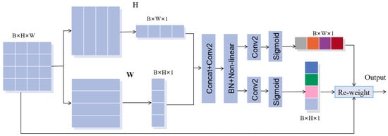
Figure 4.
The architecture of the coordinate attention.
First, the input is processed by the CA module, which converts it into two separate vectors using two-dimension global pooling. This operation encodes each channel along the two spatial directions using average pooling cores of sizes (H, 1) and (1, W), respectively.
The output of b-channel at height H can be expressed as:
Similarly, the output of channel b at width W can be expressed as:
After the two transforms are generated, feature aggregation is carried out along two spatial directions. The two transformed vectors are concatenated and passed through the 1 × 1 convolution transformation function to generate an intermediate feature map , which captures the spatial information of the horizontal and vertical directions. The parameter r represents the reduction ratio, and the function f can be expressed as:
Next, we divide the function f into two separate tensors and along the two spatial directions. The resulting feature maps are then transformed using two 1 × 1 2-D convolution operations, enabling them to be brought to the same channel number as the original input X; the formula is as follows:
where is the sigmoid function. And then, and are then expanded and used as the attention weights of the H and W direction, respectively. The final output of the coordinate attention module can be defined as:
3. Experiments
In this section, we conduct experiments on three classical public datasets: the Indian Pines, the Pavia University, and the Salinas datasets to evaluate the performance of our proposed method. We compare our method with several existing methods, including SVM [8], FDSSC [21], SSRN [20], HybridSN [31], CGCNN [32], DBMA [33], and DBDA [29]. We evaluate the effectiveness of our proposed method using overall accuracy (OA), average accuracy (AA), and Kappa statistics (KPP). OA measures the overall accuracy of a classification model, which is defined as the proportion of correctly classified samples in the entire test set. AA is the average accuracy per class, which considers the accuracy of the model for each class. Kappa index is a measure of agreement between the predicted and true class labels that considers the agreement that could occur by chance. The kappa index can be calculated from the confusion matrix, and it is widely used in multi-class classification problems to evaluate the performance of a classifier.
3.1. Configuration for Parameters
The proposed MSSCA method comprises of four modules: PCN, M-MHSA, SA, and CA. Specifically, the PCN module utilizes two network layers and 128 1×1 convolution kernels, and the activation functions used in PCN are leaky rectified linear units (Leaky ReLUs). In the M-MHSA, the numbers of the heads are set to four, and we reduce the spatial dimensions of K and V from (H×W) to (16×16). We adopt a learning rate of 0.005 for iterative updating, and the maximum number of iterations is set to 600. Finally, we conduct experiments on an NVIDIA Geforce RTX 3090 computer with 16 GB of RAM. The experiments were carried out on a Windows 10 Home Edition platform, and the code was implemented using Python 3.7.13 and PyTorch 1.11.0.
3.2. HSI Datasets
- (1)
- Indian Pines dataset: The first dataset is the Indian Pines dataset acquired by the imaging spectrometer AVIRIS in northwest Indiana, USA. The HSI of this scene consists of 145 × 145 pixels, with 220 bands and a spatial resolution of 20 m/pixel. After removing interference bands, the dataset includes 200 available bands. The dataset comprises 16 different categories of ground objects, with 10,249 reference samples. For training, validation, and testing purposes, 10%, 1%, and 89% of each category were randomly selected, respectively. Figure 5 displays the false-color image and real map, while Table 1 provides detailed category information for this HSI dataset.
- (2)
- Pavia University dataset: The second dataset is the Pavia University dataset acquired at the Pavia University using the Imaging Spectrometer Sensor ROSIS of the Reflexology System. The HSI of this scene comprises 610 × 340 pixels, with 115 bands and a spatial resolution of 1.3 m/pixel. After removing the interference bands, the dataset includes 103 available bands. The dataset contains nine different categories of ground objects, with 42,776 reference samples. For training, verification, and testing purposes, 1%, 1%, and 98% of each category’s samples were randomly selected, respectively. Figure 6 displays the false-color image and real map, while Table 2 provides detailed class information for this HSI dataset.
- (3)
- Salinas dataset: The third dataset is the Salinas dataset acquired by the AVIRIS Imaging Spectrometer sensor over the Salinas Valley. The HSI of the scene comprises 512 × 217 pixels, with 224 bands and a spatial resolution of 3.7 m/pixel. After discarding 20 interference bands, the dataset includes 204 available bands. The dataset contains 16 different categories of features, with 54,129 samples available for the experiment. For training, verification, and testing purposes, 1%, 1%, and 98% of each category’s samples were randomly selected, respectively. Figure 7 displays the false-color image and the real object map, while Table 3 provides detailed class information for this HSI dataset.

Figure 5.
Indian Pines images: (a) false-color image; (b) ground truth.


Table 1.
Category information of Indian Pines Dataset.

Figure 6.
Pavia University images: (a) false-color image; (b) ground truth.

Table 2.
Category information of Pavia University dataset.

Figure 7.
Salinas images: (a) false-color image; (b) ground truth.

Table 3.
Category information of Salinas dataset.
3.3. Comparison of Classification Results
In this section, we evaluate the performance of our proposed method and compare it with several deep learning-based networks on three datasets. We conducted 10 repeated experiments and report the experimental results as mean ± standard deviation. The classification accuracy of different classification methods on each dataset is presented in Table 4, Table 5 and Table 6. Additionally, we display the classification maps obtained by these methods in Figure 8, Figure 9 and Figure 10.
Table 4.
Classification performance of different methods on the Indian Pines dataset.
Table 5.
Classification performance of different methods on the Pavia University dataset.
Table 6.
Classification performance of different methods on the Salinas dataset.
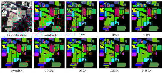
Figure 8.
Classification maps of different methods for the Indian Pines dataset.
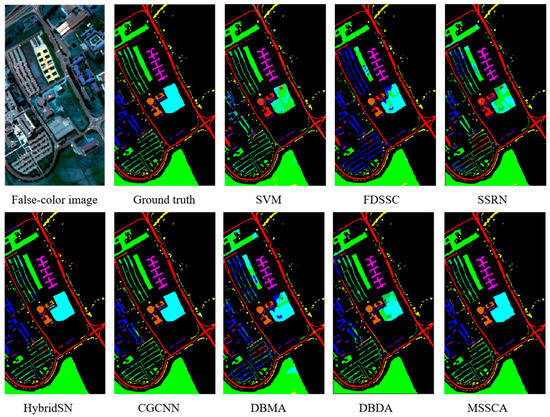
Figure 9.
Classification maps of different methods for the Pavia University dataset.
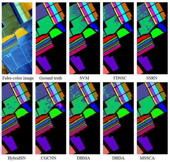
Figure 10.
Classification maps of different methods for the Salinas dataset.
Experiments on the Indian Pines dataset demonstrate that our proposed method achieves the highest classification accuracy compared to other methods. The SSRN network extracts spectral and spatial features through continuous spectral and spatial residual blocks, respectively, effectively alleviating the gradient descent phenomenon. Compared to traditional methods, it has shown significant improvement. Our proposed method further improves the accuracy by incorporating an attention mechanism, which has been shown to be more effective than that of SSRN. As shown in Table 4, the proposed method improves the overall accuracy by 25.84% and 15.10% compared to DBMA and DBDA, respectively. Moreover, it also surpasses the advanced CNN network CGCNN.
As shown in Figure 8, our proposed method has fewer misclassification points, which is more consistent with the ground truth. In contrast, the traditional SVM method produces a lot of salt and pepper noise, resulting in many misclassifications. By combining spectral and coordinate attention, our network focuses on effective information, resulting in a significant reduction in the error rate and smoother classification maps.
Similar to the results on the Indian Pines dataset, our proposed method achieves the best classification results on the Pavia University dataset compared to other methods, demonstrating the stability of our network. As shown in Table 5, our proposed method outperforms current state-of-the-art methods, such as CGCNN, DBMA, and DBDA, by improving OA by 1.05%, 15.81%, and 7.16%, respectively. Moreover, our proposed MSSCA method achieves an accuracy of 95% in each category, indicating its effectiveness.
Figure 9 shows that our proposed MSSCA method has fewer misclassification points on the Pavia University dataset, which is more consistent with the ground truth compared to CGCNN, which has shown good performance on this dataset.
Table 6 presents the classification results on the Salinas dataset, where our proposed MSSCA method achieves the best overall accuracy (OA), average accuracy (AA), and Kappa statistics (KPP), with an OA accuracy of 99.41%. Moreover, our proposed method achieves almost the best classification results in each category.
The classification results of different methods on the Salinas dataset are shown in Figure 10, where our proposed MSSCA method outperforms other methods in misclassified categories, such as Lettuce_romaine_7 wk and Vinyard_untrained. The classification map generated by our method is more consistent with the ground truth, and the class boundaries are clearer.
3.4. Ablation Study
To evaluate the effectiveness of each module in the MSSCA architecture, we conducted a set of ablation experiments by splitting and combining different network modules. Table 7 presents the classification accuracy of different modules. As can be seen from the table, using only the SE or CA module results in lower OA compared to when both modules are combined. This indicates that the addition of both SE and CA modules improves the classification accuracy. The SE module focuses on the importance of channels, while the CA module focuses on the importance of spatial locations. By paying attention to both channel and coordinate information, the model can more effectively utilize relevant information, resulting in improved classification results. Moreover, incorporating the PCN module improves classification accuracy by providing more discriminative input and optimizing network feature modules.
Table 7.
Ablation study on attention modules (OA%).
3.5. Training Sample Ratio
As is well known, deep learning algorithms heavily depend on large amounts of high-quality labeled data, and the network performance improves as the quantity of labeled data increases. In this section, we analyze the comparative results of different training ratios. Figure 11 presents the experimental results. For the Indian Pines dataset, we use 0.5%, 1%, 3%, 5%, and 10% samples as the training sets. For PU and SV datasets, we use 0.1%, 0.5%, 1%, 5%, and 10%, respectively.
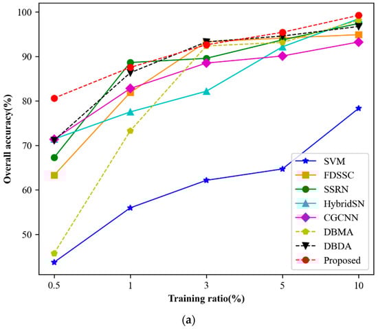
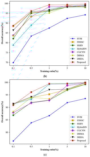
Figure 11.
The OA of different methods with varying ratios of training samples. (a) Indian Pines. (b) Pavia University. (c) Salinas.
As shown in Figure 11a–c, the classification accuracy of all three datasets increases as the training ratio increases. With sufficient training samples, almost perfect classification results can be achieved. Moreover, as the training ratio increases, the difference in classification accuracy between different methods becomes smaller. Notably, even with a small training ratio, our proposed MSSCA method outperforms other comparison methods. The performance of our proposed method exhibits a steady growth trend across all three datasets, indicating its effectiveness and stability.
3.6. Running Time
This section presents the training and testing times of different methods on different datasets, as shown in Table 8, Table 9 and Table 10. Since the goal of HSI classification is to assign a specific label to each pixel, we consider the time taken to classify all pixels as the test time. From the tables, we can see that SVM has a short training time, but it can only extract shallow features and has poor classification performance. Existing deep learning methods such as DBMA and DBDA perform well but have long testing times. In contrast, our proposed MSSCA method not only achieves outstanding classification performance, but also has a short testing time and low computational cost. This is because we use a lightweight attention mechanism, which reduces the computational cost while improving performance.
Table 8.
Running time (s) of different methods on the Indian Pines dataset.
Table 9.
Running time (s) of different methods on the Pavia University dataset.
Table 10.
Running time (s) of different methods on the Salinas dataset.
4. Conclusions
In this paper, we propose an effective deep learning method called MSSCA for HSI classification. In MSSCA, to reduce the computational burden caused by the dot-product operation, the down-sampling operation is introduced into MHSA, and the novel M-MHSA is proposed to depict the long-range dependencies of HSI pixels. On this basis, we integrate SE and CA networks to effectively leverage spectral and spatial coordinate information, which enhances network performance and classification results without compromising network complexity or computational costs. Three classical datasets, including Indian Pines, Pavia University, and Salinas, are used to evaluate the proposed method. The proposed method’s performance was validated by a performance comparison with some classical methods, such as SSRN, HybridSN, and DBDA. The proposed MSSCA method achieved an overall accuracy of 99.96% for Indian Pines datasets, 99.26% for Pavia University datasets, and 99.41% for Salinas datasets, outperforming most existing HSI classification methods, highlighting the effectiveness and efficiency of our proposed method in HSI classification. In the future, we will continue to explore more lightweight and effective classification frameworks to HSI classification under complex conditions.
Author Contributions
Methodology, M.Z. and Y.D.; validation, Y.D.; writing—original draft preparation, Y.D.; writing—review and editing, M.Z., Y.D., W.S. and H.M.; supervision, M.Z., W.S. and H.M.; funding acquisition, W.S. and Q.H. All authors have read and agreed to the published version of the manuscript.
Funding
This work was funded by the National Natural Science Foundation of China (61972240), and the Shanghai Science and Technology Commission part of the local university capacity building projects (20050501900).
Institutional Review Board Statement
Not applicable.
Informed Consent Statement
Not applicable.
Data Availability Statement
All data used in this paper are available at https://ehu.eus/ccwintco/index.php/Hyperspectral_Remote_Sensing_Scenes, accessed on 10 April 2022.
Acknowledgments
We thank the reviewers and editors for their professional suggestions.
Conflicts of Interest
The authors declare no conflict of interest.
References
- Govender, M.; Chetty, K.; Naiken, V.; Bulcock, H. A comparison of satellite hyperspectral and multispectral remote sensing imagery for improved classification and mapping of vegetation. Water Sa 2019, 34, 147–154. [Google Scholar] [CrossRef]
- Govender, M.; Chetty, K.; Bulcock, H. A review of hyperspectral remote sensing and its application in vegetation and water resource studies. Water Sa 2009, 33, 145–151. [Google Scholar] [CrossRef]
- Khan, M.J.; Khan, H.S.; Yousaf, A.; Khurshid, K.; Abbas, A. Modern Trends in Hyperspectral Image Analysis: A Review. IEEE Access 2018, 6, 14118–14129. [Google Scholar] [CrossRef]
- Huang, H.; Liu, L.; Ngadi, M. Recent Developments in Hyperspectral Imaging for Assessment of Food Quality and Safety. Sensors 2014, 14, 7248–7276. [Google Scholar] [CrossRef] [PubMed]
- Blanzieri, E.; Melgani, F. Nearest Neighbor Classification of Remote Sensing Images with the Maximal Margin Principle. IEEE Trans. Geosci. Remote Sens. 2008, 46, 1804–1811. [Google Scholar] [CrossRef]
- Amini, A.; Homayouni, S.; Safari, A. Semi-supervised classification of hyperspectral image using random forest algorithm. In Proceedings of the 2014 IEEE Geoscience and Remote Sensing Symposium, Quebec City, QC, Canada, 13–18 July 2014; pp. 2866–2869. [Google Scholar] [CrossRef]
- Li, S.; Jia, X.; Zhang, B. Superpixel-based Markov random field for classification of hyperspectral images. In Proceedings of the 2013 IEEE International Geoscience and Remote Sensing Symposium—IGARSS, Melbourne, Australia, 21–26 July 2013; pp. 3491–3494. [Google Scholar] [CrossRef]
- Melgani, F.; Bruzzone, L. Classification of hyperspectral remote sensing images with support vector machines. IEEE Trans. Geosci. Remote Sens. 2004, 42, 1778–1790. [Google Scholar] [CrossRef]
- Qi, Y.; Wang, Y.; Zheng, X.; Wu, Z. Robust feature learning by stacked autoencoder wit-h maximum correntropy criterion. In Proceedings of the 2014 IEEE International Conference on Acoustics, Speech and Signal Processing (ICASSP), Florence, Italy, 4–9 May 2014; pp. 6716–6720. [Google Scholar] [CrossRef]
- Mou, L.; Ghamisi, P.; Zhu, X.X. Deep Recurrent Neural Networks for Hyperspectral Image Classification. IEEE Trans. Geosci. Remote Sens. 2017, 55, 3639–3655. [Google Scholar] [CrossRef]
- Mughees, A.; Tao, L. Multiple deep-belief-network-based spectral-spatial classification of hyperspectral images. Tsinghua Sci. Technol. 2019, 24, 183–194. [Google Scholar] [CrossRef]
- Zheng, Z.; Zhang, Y.; Li, L.; Zhu, M.; He, Y.; Li, M.; Guo, Z.; Yang, X.; Liu, X. Classification based on deep convolutional neural networks with hyperspectral image. In Proceedings of the 2017 IEEE International Geoscience and Remote Sensing Symposium (IGARSS), Fort Worth, TX, USA, 23–28 July 2017; pp. 1828–1831. [Google Scholar] [CrossRef]
- Ma, C.; Guo, M.Y. Hyperspectral Image Classification Based on Convolutional Neural Network. In Proceedings of the 2018 5th International Conference on Information, Cybernetics, and Computational Social Systems (ICCSS), Hangzhou, China, 16–19 August 2018; pp. 117–121. [Google Scholar] [CrossRef]
- Dai, X.; Xue, W. Hyperspectral Remote Sensing Image Classification Based on Convolutional Neural Network. In Proceedings of the 2018 37th Chinese Control Conference (CCC), Wuhan, China, 25–27 July 2018; pp. 10373–10377. [Google Scholar] [CrossRef]
- Chen, Y.; Lin, Z.; Zhao, X.; Wang, G.; Gu, Y. Deep Learning-Based Classification of Hyperspectral Data. IEEE J. Sel. Top. Appl. Earth Obs. Remote Sens. 2014, 7, 2094–2107. [Google Scholar] [CrossRef]
- Hu, W.; Huang, Y.; Wei, L.; Zhang, F.; Li, H. Deep Convolutional Neural Networks f-or Hyperspectral Image Classification. J. Sens. 2015, 2015, 258619. [Google Scholar] [CrossRef]
- Li, Y.; Zhang, H.; Shen, Q. Spectral—Spatial Classification of Hyperspectral Imagery with 3D Convolutional Neural Network. Remote Sens. 2017, 9, 67. [Google Scholar] [CrossRef]
- Yang, J.; Zhao, Y.Q.; Chan, W.C. Learning and Transferring Deep Joint Spectral—Spatial Features for Hyperspectral Classification. IEEE Trans. Geosci. Remote Sens. 2017, 55, 4729–4742. [Google Scholar] [CrossRef]
- Chen, C.; Zhang, J.J.; Zheng, C.H.; Yan, Q.; Xun, L.N. Classification of Hyperspectral Data Using a Multi-Channel Convolutional Neural Network. In Proceedings of the Intelligent Computing Methosologies; Huang, D.S., Gromiha, M.M., Han, K., Hussain, A., Eds.; Springer International Publishing: Cham, Switzerlands, 2018; pp. 81–92. [Google Scholar] [CrossRef]
- Zhong, Z.; Li, J.; Luo, Z.; Chapman, M. Spectral–Spatial Residual Network for Hyperspectral Image Classification: A 3-D Deep Learning Framework. IEEE Trans. Geosci. Remote Sens. 2018, 56, 847–858. [Google Scholar] [CrossRef]
- Wang, W.; Dou, S.; Jiang, Z.; Sun, L. A Fast Dense Spectral—Spatial Convolution Network Framework for Hyperspectral Images Classification. Remote Sens. 2018, 10, 1068. [Google Scholar] [CrossRef]
- He, K.; Zhang, X.; Ren, S.; Sun, J. Deep Residual Learning for Image Recognition. In Proceedings of the 2016 IEEE Conference on Computer Vision and Pattern Recognition (CVPR), Las Vegas, NV, USA, 27–30 June 2016; pp. 770–778. [Google Scholar]
- Huang, G.; Liu, Z.; Maaten, L.V.D.; Weinberger, K.Q. Densely Connected Convolutional Networks. In Proceedings of the IEEE Conference on Computer Vision and Pattern Recognition (CVPR) 2017, Honolulu, HI, USA, 21–26 July 2017; pp. 2261–2269. [Google Scholar]
- Qin, A.; Shang, Z.; Tian, J.; Wang, Y.; Zhang, T.; Tang, Y.Y. Spectral-Spatial Graph Convolutional Networks for Semel-Supervised Hyperspectral Image Classification. IEEE Trans. Geosci. Remote Sens. Lett. 2019, 16, 241–245. [Google Scholar] [CrossRef]
- Vaswani, A.; Shazeer, N.; Parmar, N.; Uszkoreit, J.; Jones, L.; Gomez, A.N.; Kaiser, L.; Polosukhin, I. Attention Is All You Need. Adv. Neural Inf. Process. Syst. 2017, 30, 2–8. Available online: http://arxiv.org/abs/1706.03762v5 (accessed on 15 June 2023).
- Song, C.; Mei, S.; Ma, M.; Xu, F.; Zhang, Y.; Du, Q. Hyperspectral Image Classification Using Hierarchical Spatial-Spectral Transformer. In Proceedings of the IGARSS 2022—2022 IEEE International Geoscience and Remote Sensing Symposium, Kuala Lumpur, Malaysia, 17–22 July 2022; pp. 3584–3587. [Google Scholar] [CrossRef]
- Valsalan, P.; Latha, G.C.P. Hyperspectral image classification model using squeeze and excitation network with deep learning. Comput. Intell. Neurosci. 2022, 2022, 9430779. [Google Scholar] [CrossRef]
- Sun, H.; Zheng, X.; Lu, X.; Wu, S. Spectral—Spatial Attention Network for Hyperspectral Image Classification. IEEE Trans. Geosci. Remote Sens. 2020, 58, 3232–3245. [Google Scholar] [CrossRef]
- Li, R.; Zheng, S.; Duan, C.; Yang, Y.; Wang, X. Classification of Hyperspectral Image Based on Double-Branch Dual-Attention Mechanism Network. Remote Sens. 2020, 12, 582. [Google Scholar] [CrossRef]
- Hou, Q.; Zhou, D.; Feng, J. Coordinate Attention for Efficient Mobile Network Design. In Proceedings of the IEEE/CVF Conference on Computer Vision and Pattern Recognition, Nashville, TN, USA, 20–25 June 2021. [Google Scholar] [CrossRef]
- Roy, S.K.; Krishna, G.; Dubey, S.R.; Chaudhuri, B.B. HybridSN: Exploring 3-D—2-D CNN Feature Hierarchy for Hyperspectral Image Classification. IEEE Trans. Geosci. Remote Sens. 2020, 17, 277–281. [Google Scholar] [CrossRef]
- Liu, Q.; Xiao, L.; Yang, J.; Chan, J.C. Content-Guided Convolutional Neural Network for Hyperspectral Image Classification. IEEE Trans. Geosci. Remote Sens. 2020, 58, 6124–6137. [Google Scholar] [CrossRef]
- Ma, W.; Yang, Q.; Wu, Y.; Zhao, W.; Zhang, X. Double-Branch Multi-Attention Mechanism Network for Hyperspectral Image Classification. Remote Sens. 2019, 11, 1307. [Google Scholar] [CrossRef]


Disclaimer/Publisher’s Note: The statements, opinions and data contained in all publications are solely those of the individual author(s) and contributor(s) and not of MDPI and/or the editor(s). MDPI and/or the editor(s) disclaim responsibility for any injury to people or property resulting from any ideas, methods, instructions or products referred to in the content. |
© 2023 by the authors. Licensee MDPI, Basel, Switzerland. This article is an open access article distributed under the terms and conditions of the Creative Commons Attribution (CC BY) license (https://creativecommons.org/licenses/by/4.0/).