
Future Prediction of Shuttlecock Trajectory in Badminton Using Player’s Information


Abstract
1. Introduction
- This is a pioneering study on predicting the trajectory of the badminton shuttlecock during a match.
- The proposed method predicts the shuttlecock’s trajectory by considering the player’s position and posture information, in addition to the shuttlecock’s position information.
- The results of the experiments show that the proposed method outperforms previous methods that use only shuttlecock position information as input or methods that use both shuttlecock and player position information as input.
2. Materials and Methods
2.1. Related Work
2.1.1. Future Predictions in Net Sports
2.1.2. Object Detection
2.1.3. Pose Estimation
2.2. Method
2.2.1. Overview
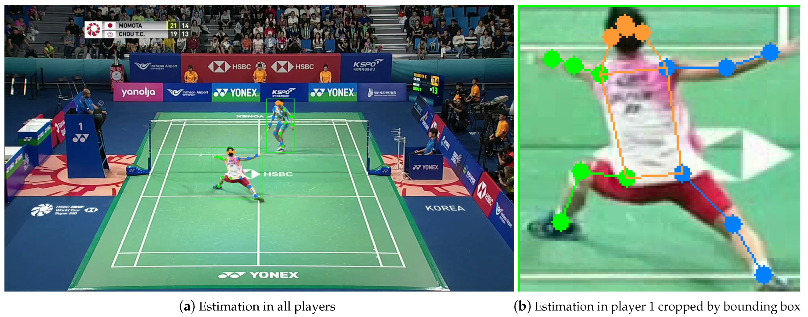
2.2.2. Detection and Pose Estimation from Past Frames
2.2.3. Time Series Model for Future Prediction
2.3. Experiment
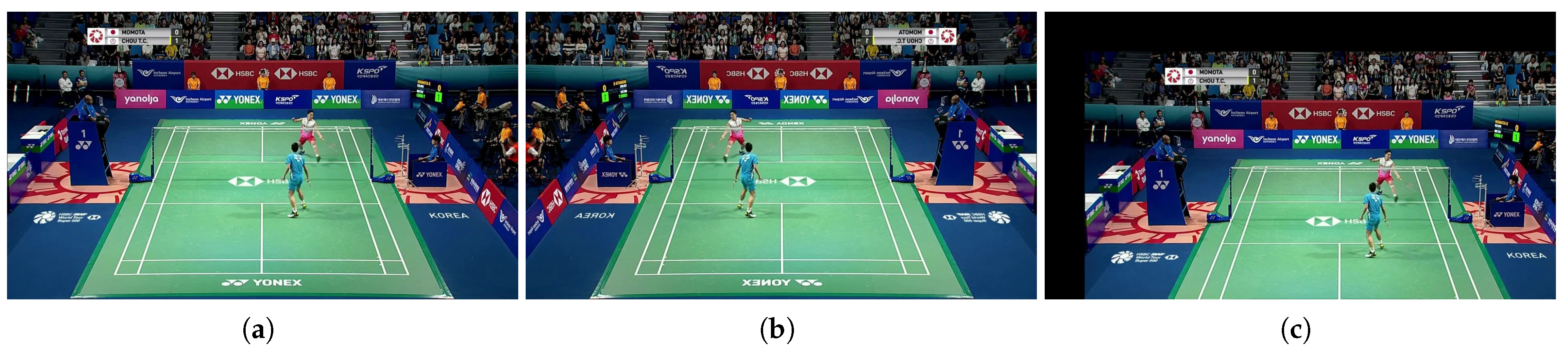
2.3.1. Dataset
2.3.2. Evaluation Metrics
2.3.3. Network Training
2.3.4. Other Models
Baseline Models
Other Time-Series Models
Other Representations of Posture Information
2.3.5. Data Augmentation Values
2.3.6. The Number of Frames of Past/Future
3. Results
3.1. Comparison with Other Models
3.2. Comparison by Data Augmentation Values
3.3. Comparison of the Number of Frames of Past/Future
4. Discussion and Conclusions
4.1. Limitation
4.2. Future Work
4.3. Conclusions
Author Contributions
Funding
Institutional Review Board Statement
Informed Consent Statement
Data Availability Statement
Conflicts of Interest
References
- Sun, K.; Xiao, B.; Liu, D.; Wang, J. Deep High-Resolution Representation Learning for Human Pose Estimation. In Proceedings of the IEEE Conference on Computer Vision and Pattern Recognition (CVPR), Long Beach, CA, USA, 15–20 June 2019; pp. 5686–5696. [Google Scholar] [CrossRef]
- Cao, Z.; Liao, T.; Song, W.; Chen, Z.; Li, C. Detecting the shuttlecock for a badminton robot: A YOLO based approach. Expert Syst. Appl. 2021, 164, 113833. [Google Scholar] [CrossRef]
- Waghmare, G.; Borkar, S.; Saley, V.; Chinchore, H.; Wabale, S. Badminton shuttlecock detection and prediction of trajectory using multiple 2 dimensional scanners. In Proceedings of the IEEE First International Conference on Control, Measurement and Instrumentation (CMI), Kolkata Section, India, 8–10 January 2016; pp. 234–238. [Google Scholar] [CrossRef]
- Wu, E.; Perteneder, F.; Koike, H. Real-time Table Tennis Forecasting System based on Long Short-term Pose Prediction Network. In Proceedings of the SIGGRAPH Asia Posters (SA), Brisbane, Australia, 17–20 November 2019; pp. 23:1–23:2. [Google Scholar] [CrossRef]
- Wu, E.; Koike, H. FuturePong: Real-time table tennis trajectory forecasting using pose prediction network. In Proceedings of the Extended Abstracts of the 2020 CHI Conference on Human Factors in Computing Systems (CHI EA), Honolulu, HI, USA, 25–30 April 2020; pp. 1–8. [Google Scholar] [CrossRef]
- Sato, K.; Sano, Y.; Otsuki, M.; Oka, M.; Kato, K. Augmented Recreational Volleyball Court: Supporting the Beginners’ Landing Position Prediction Skill by Providing Peripheral Visual Feedback. In Proceedings of the 10th Augmented Human International Conference (AH), Reims, France, 11–12 March 2019; Wolf, K., Zhang, H., Taïar, R., Seigneur, J.M., Eds.; ACM: New York, NY, USA, 2019; pp. 15:1–15:9. [Google Scholar]
- Fernando, T.; Denman, S.; Sridharan, S.; Fookes, C. Memory Augmented Deep Generative models for Forecasting the Next Shot Location in Tennis. IEEE Trans. Knowl. Data Eng. 2019, 32, 1785–1797. [Google Scholar] [CrossRef]
- Wang, W.Y.; Shuai, H.H.; Chang, K.S.; Peng, W.C. ShuttleNet: Position-Aware Fusion of Rally Progress and Player Styles for Stroke Forecasting in Badminton. In Proceedings of the AAAI Conference on Artificial Intelligence (AAAI), Virtual, 22 February–1 March 2022; Volume 36, pp. 4219–4227. [Google Scholar] [CrossRef]
- Rumelhart, D.E.; Hinton, G.E.; Williams, R.J. Learning representations by back-propagating errors. Nature 1986, 323, 533–536. [Google Scholar] [CrossRef]
- Ik, T.U. Shuttlecock Trajectory Dataset. 2020. Available online: https://hackmd.io/Nf8Rh1NrSrqNUzmO0sQKZw (accessed on 1 January 2020).
- Shimizu, T.; Hachiuma, R.; Saito, H.; Yoshikawa, T.; Lee, C. Prediction of Future Shot Direction using Pose and Position of Tennis Player. In Proceedings of the 2nd International Workshop on Multimedia Content Analysis in Sports (MMSports), Nice, France, 25 October 2019; pp. 59–66. [Google Scholar] [CrossRef]
- Suda, S.; Makino, Y.; Shinoda, H. Prediction of Volleyball Trajectory Using Skeletal Motions of Setter Player. In Proceedings of the 10th Augmented Human International Conference (AH), Reims, France, 11–12 March 2019; pp. 16:1–16:8. [Google Scholar] [CrossRef]
- Lin, H.I.; Yu, Z.; Huang, Y.C. Ball Tracking and Trajectory Prediction for Table-Tennis Robots. Sensors 2020, 20, 333. [Google Scholar] [CrossRef] [PubMed]
- Denton, E.L.; Gross, S.; Fergus, R. Semi-Supervised Learning with Context-Conditional Generative Adversarial Networks. arXiv 2016, arXiv:1611.06430. [Google Scholar]
- Redmon, J.; Divvala, S.K.; Girshick, R.B.; Farhadi, A. You Only Look Once: Unified, Real-Time Object Detection. In Proceedings of the IEEE Conference on Computer Vision and Pattern Recognition (CVPR), Las Vegas, NV, USA, 27–30 June 2016; IEEE Computer Society: New York, NY, USA, 2016; pp. 779–788. [Google Scholar]
- Liu, W.; Anguelov, D.; Erhan, D.; Szegedy, C.; Reed, S.; Fu, C.Y.; Berg, A.C. SSD: Single Shot MultiBox Detector. In Proceedings of the European Conference on Computer Vision (ECCV), Amsterdam, The Netherlands, 11–14 October 2016; Leibe, B., Matas, J., Sebe, N., Welling, M., Eds.; Springer International Publishing: Cham, Switzerland, 2016; pp. 21–37. [Google Scholar]
- Bochkovskiy, A.; Wang, C.; Liao, H.M. YOLOv4: Optimal Speed and Accuracy of Object Detection. arXiv 2020, arXiv:2004.10934. [Google Scholar]
- Girshick, R.; Donahue, J.; Darrell, T.; Malik, J. Rich Feature Hierarchies for Accurate Object Detection and Semantic Segmentation. In Proceedings of the IEEE Conference on Computer Vision and Pattern Recognition (CVPR), Columbus, OH, USA, 23–28 June 2014; pp. 580–587. [Google Scholar] [CrossRef]
- Girshick, R. Fast R-CNN. In Proceedings of the IEEE International Conference on Computer Vision (ICCV), Santiago, Chile, 7–13 December 2015; pp. 1440–1448. [Google Scholar]
- Ren, S.; He, K.; Girshick, R.; Sun, J. Faster R-CNN: Towards Real-Time Object Detection with Region Proposal Networks. In Proceedings of the Advances in Neural Information Processing Systems (NIPS), Montreal, QC, Canada, 7–12 December 2015; Volume 28, pp. 91–99. [Google Scholar]
- Toshev, A.; Szegedy, C. DeepPose: Human Pose Estimation via Deep Neural Networks. In Proceedings of the IEEE Conference on Computer Vision and Pattern Recognition (CVPR), Columbus, OH, USA, 23–28 June 2014; IEEE Computer Society: New York, NY, USA, 2014; pp. 1653–1660. [Google Scholar]
- Tompson, J.; Jain, A.; LeCun, Y.; Bregler, C. Joint Training of a Convolutional Network and a Graphical Model for Human Pose Estimation. In Proceedings of the Conference on Neural Information Processing System (NIPS), Montreal, QC, Canada, 8–13 December 2014; Ghahramani, Z., Welling, M., Cortes, C., Lawrence, N.D., Weinberger, K.Q., Eds.; Curran Associates, Inc.: Red Hook, NY, USA, 2014; pp. 1799–1807. [Google Scholar]
- Wei, S.E.; Ramakrishna, V.; Kanade, T.; Sheikh, Y. Convolutional Pose Machines. In Proceedings of the IEEE Conference on Computer Vision and Pattern Recognition (CVPR), Las Vegas, NV, USA, 27–30 June 2016; IEEE Computer Society: New York, NY, USA, 2016; pp. 4724–4732. [Google Scholar]
- Newell, A.; Yang, K.; Deng, J. Stacked Hourglass Networks for Human Pose Estimation. In Proceedings of the European Conference on Computer Vision (ECCV), Amsterdam, The Netherlands, 11–14 October 2016; Leibe, B., Matas, J., Sebe, N., Welling, M., Eds.; Springer International Publishing: Cham, Switzerland, 2016; pp. 483–499. [Google Scholar]
- Chen, Y.; Wang, Z.; Peng, Y.; Zhang, Z.; Yu, G.; Sun, J. Cascaded Pyramid Network for Multi-Person Pose Estimation. In Proceedings of the IEEE Conference on Computer Vision and Pattern Recognition (CVPR), Salt Lake City, UT, USA, 18–23 June 2018; IEEE Computer Society: New York, NY, USA, 2018; pp. 7103–7112. [Google Scholar]
- Xiao, B.; Wu, H.; Wei, Y. Simple Baselines for Human Pose Estimation and Tracking. In Lecture Notes in Computer Science, Proceedings of the European Conference on Computer Vision (ECCV), Munich, Germany, 8–14 September 2018; Ferrari, V., Hebert, M., Sminchisescu, C., Weiss, Y., Eds.; Springer: Berlin/Heidelberg, Germany, 2018; Volume 11210, pp. 472–487. [Google Scholar]
- Duan, H.; Lin, K.Y.; Jin, S.; Liu, W.; Qian, C.; Ouyang, W. TRB: A Novel Triplet Representation for Understanding 2D Human Body. In Proceedings of the IEEE International Conference on Computer Vision (ICCV), Seoul, Republic of Korea, 27 October–2 November 2019; pp. 9478–9487. [Google Scholar]
- Pishchulin, L.; Insafutdinov, E.; Tang, S.; Andres, B.; Andriluka, M.; Gehler, P.V.; Schiele, B. DeepCut: Joint Subset Partition and Labeling for Multi Person Pose Estimation. In Proceedings of the IEEE Conference on Computer Vision and Pattern Recognition (CVPR), Las Vegas, NV, USA, 27–30 June 2016; IEEE Computer Society: New York, NY, USA, 2016; pp. 4929–4937. [Google Scholar]
- Insafutdinov, E.; Pishchulin, L.; Andres, B.; Andriluka, M.; Schiele, B. DeeperCut: A Deeper, Stronger, and Faster Multi-person Pose Estimation Model. In Lecture Notes in Computer Science, Proceedings of the European Conference on Computer Vision (ECCV), Amsterdam, The Netherlands, 11–14 October 2016; Leibe, B., Matas, J., Sebe, N., Welling, M., Eds.; Springer: Berlin/Heidelberg, Germany, 2016; Volume 9910, pp. 34–50. [Google Scholar]
- Cao, Z.; Simon, T.; Wei, S.E.; Sheikh, Y. Realtime Multi-person 2D Pose Estimation Using Part Affinity Fields. In Proceedings of the IEEE Conference on Computer Vision and Pattern Recognition (CVPR), Honolulu, HI, USA, 21–16 July 2017; IEEE Computer Society: New York, NY, USA, 2017; pp. 1302–1310. [Google Scholar]
- Newell, A.; Huang, Z.; Deng, J. Associative Embedding: End-to-End Learning for Joint Detection and Grouping. In Proceedings of the Conference on Neural Information Processing System (NIPS), Long Beach, CA, USA, 4–9 December 2017; Guyon, I., von Luxburg, U., Bengio, S., Wallach, H.M., Fergus, R., Vishwanathan, S.V.N., Garnett, R., Eds.; Curran Associates, Inc.: Red Hook, NY, USA, 2017; pp. 2277–2287. [Google Scholar]
- Papandreou, G.; Zhu, T.; Chen, L.C.; Gidaris, S.; Tompson, J.; Murphy, K. PersonLab: Person Pose Estimation and Instance Segmentation with a Bottom-Up, Part-Based, Geometric Embedding Model. In Lecture Notes in Computer Science, Proceedings of the European Conference on Computer Vision (ECCV), Munich, Germany, 8–14 September 2018; Ferrari, V., Hebert, M., Sminchisescu, C., Weiss, Y., Eds.; Springer: Berlin/Heidelberg, Germany, 2018; Volume 11218, pp. 282–299. [Google Scholar]
- Martinez, G.H.; Raaj, Y.; Idrees, H.; Xiang, D.; Joo, H.; Simon, T.; Sheikh, Y. Single-Network Whole-Body Pose Estimation. In Proceedings of the IEEE International Conference on Computer Vision (ICCV), Seoul, Republic of Korea, 27 October–2 November 2019; pp. 6981–6990. [Google Scholar]
- Huang, Y.C.; Liao, I.N.; Chen, C.H.; İk, T.U.; Peng, W.C. TrackNet: A Deep Learning Network for Tracking High-speed and Tiny Objects in Sports Applications. In Proceedings of the 16th IEEE International Conference on Advanced Video and Signal Based Surveillance (AVSS), Taipei, Taiwan, 18–21 September 2019; pp. 1–8. [Google Scholar] [CrossRef]
- Sengupta, A.; Jin, F.; Zhang, R.; Cao, S. mm-Pose: Real-Time Human Skeletal Posture Estimation Using mmWave Radars and CNNs. IEEE Sens. J. 2020, 20, 10032–10044. [Google Scholar] [CrossRef]
- Lin, T.Y.; Maire, M.; Belongie, S.J.; Hays, J.; Perona, P.; Ramanan, D.; Dollár, P.; Zitnick, C.L. Microsoft COCO: Common Objects in Context. In Proceedings of the European Conference on Computer Vision (ECCV), Zurich, Switzerland, 6–12 September 2014; Volume 8693, pp. 740–755. [Google Scholar]
- Hochreiter, S.; Schmidhuber, J. Long Short-Term Memory. Neural Comput. 1997, 9, 1735–1780. [Google Scholar] [CrossRef] [PubMed]
- Sun, N.E.; Lin, Y.C.; Chuang, S.P.; Hsu, T.H.; Yu, D.R.; Chung, H.Y.; İk, T.U. TrackNetV2: Efficient Shuttlecock Tracking Network. In Proceedings of the International Conference on Pervasive Artificial Intelligence (ICPAI), Taipei, Taiwan, 3–5 December 2020; pp. 86–91. [Google Scholar] [CrossRef]
- Paszke, A.; Gross, S.; Chintala, S.; Chanan, G.; Yang, E.; DeVito, Z.; Lin, Z.; Desmaison, A.; Antiga, L.; Lerer, A. Automatic differentiation in Pytorch. In Proceedings of the Conference on Neural Information Processing System (NIPS), Long Beach, CA, USA, 4–9 December 2017. [Google Scholar]
- Kingma, D.P.; Ba, J. Adam: A Method for Stochastic Optimization. In Proceedings of the 3rd International Conference on Learning Representations (ICLR), San Diego, CA, USA, 7–9 May 2015. [Google Scholar]
- Cho, K.; van Merrienboer, B.; Gülçehre, Ç.; Bougares, F.; Schwenk, H.; Bengio, Y. Learning Phrase Representations using RNN Encoder-Decoder for Statistical Machine Translation. arXiv 2014, arXiv:1406.1078. [Google Scholar]
- Vaswani, A.; Shazeer, N.; Parmar, N.; Uszkoreit, J.; Jones, L.; Gomez, A.N.; Kaiser, L.u.; Polosukhin, I. Attention is All you Need. In Proceedings of the Conference on Neural Information Processing System (NIPS), Long Beach, CA, USA, 4–9 December 2017; Volume 30, pp. 5998–6008. [Google Scholar]
- Sutskever, I.; Vinyals, O.; Le, Q.V. Sequence to Sequence Learning with Neural Networks. In Proceedings of the Conference on Neural Information Processing System (NIPS), Montreal, QC, Canada, 8–13 December 2014; Ghahramani, Z., Welling, M., Cortes, C., Lawrence, N.D., Weinberger, K.Q., Eds.; Curran Associates, Inc.: Red Hook, NY, USA, 2014; pp. 3104–3112. [Google Scholar]
- He, K.; Zhang, X.; Ren, S.; Sun, J. Deep Residual Learning for Image Recognition. In Proceedings of the IEEE Conference on Computer Vision and Pattern Recognition (CVPR), Las Vegas, NV, USA, 27–30 June 2016; pp. 770–778. [Google Scholar] [CrossRef]


| Year | Author | Sports | Prediction Target |
|---|---|---|---|
| 2019 | Shimizu et al. [11] | Tennis | Shot direction |
| 2016 | Waghmare et al. [3] | Badminton | Shuttlecock landing point |
| 2019, 2020 | Wu et al. [4,5] | Table tennis | Serve landing point |
| 2019 | Sato et al. [6] | Volleyball | Ball landing point |
| 2019 | Fernando et al. [7] | Tennis | Stroke |
| 2022 | Wang et al. [8] | Badminton | Stroke |
| 2019 | Suda et al. [12] | Volleyball | Toss trajectory |
| 2020 | Lin et al. [13] | Table tennis | Serve trajectory |
| 2022 | Proposed | Badminton | Shuttlecock trajectory |
| Target | Original | After Embedding |
|---|---|---|
| Shuttlecock position | 2 | 2 |
| Player position | 4 | 2 |
| Player posture | 68 | 2 |
| All | 74 | 6 |
| Models | Learning Rate |
|---|---|
| RNN | 0.005 |
| GRU | 0.01 |
| Transformer | 0.001 |
| Seq2Seq | 0.02 |
| Input Data | Models | ADE (Pixel) | |||||
|---|---|---|---|---|---|---|---|
| Shuttlecock Position | Player Position | Player Posture | Match A | Match B | Match C | Average | |
| ∘ | - | - | LSTM | 54.1 | 40.7 | 45.8 | 47.6 |
| ∘ | ∘ | - | LSTM | 51.6 | 36.5 | 43.9 | 45.2 |
| ∘ | ∘ | R | RNN | 52.0 | 38.9 | 44.9 | 45.9 |
| ∘ | ∘ | H | RNN | 63.4 | 46.0 | 60.2 | 58.4 |
| ∘ | ∘ | A | RNN | 55.4 | 38.0 | 49.8 | 48.8 |
| ∘ | ∘ | R | GRU | 48.9 | 36.1 | 42.9 | 43.6 |
| ∘ | ∘ | H | GRU | 59.8 | 42.8 | 52.9 | 51.1 |
| ∘ | ∘ | A | GRU | 53.4 | 37.0 | 43.5 | 45.4 |
| ∘ | ∘ | R | Transformer | 59.3 | 44.5 | 49.0 | 51.5 |
| ∘ | ∘ | H | Transformer | 81.0 | 65.7 | 73.4 | 74.3 |
| ∘ | ∘ | A | Transformer | 60.3 | 44.2 | 47.4 | 51.6 |
| ∘ | ∘ | R | Seq2Seq | 40.4 | 53.8 | 45.8 | 47.3 |
| ∘ | ∘ | H | Seq2Seq | 53.8 | 40.7 | 45.9 | 47.7 |
| ∘ | ∘ | A | Seq2Seq | 56.7 | 46.6 | 43.0 | 48.9 |
| ∘ | ∘ | R | LSTM | 46.5 | 34.4 | 41.0 | 41.4 |
| ∘ | ∘ | H | LSTM | 56.4 | 44.4 | 51.9 | 51.3 |
| ∘ | ∘ | A | LSTM | 48.3 | 33.0 | 39.1 | 41.4 |
| Input Data | Models | FDE (Pixel) | |||||
|---|---|---|---|---|---|---|---|
| Shuttlecock Position | Player Position | Player Posture | Match A | Match B | Match C | Average | |
| ∘ | - | - | LSTM | 94.1 | 74.1 | 75.0 | 81.5 |
| ∘ | ∘ | - | LSTM | 88.0 | 63.4 | 70.9 | 76.1 |
| ∘ | ∘ | R | RNN | 90.1 | 66.7 | 74.5 | 78.0 |
| ∘ | ∘ | H | RNN | 108.7 | 77.2 | 101.1 | 98.7 |
| ∘ | ∘ | A | RNN | 94.0 | 64.1 | 74.5 | 79.1 |
| ∘ | ∘ | R | GRU | 87.4 | 67.6 | 69.8 | 76.2 |
| ∘ | ∘ | H | GRU | 109.3 | 76.7 | 96.0 | 92.9 |
| ∘ | ∘ | A | GRU | 95.8 | 70.0 | 73.5 | 80.3 |
| ∘ | ∘ | R | Transformer | 97.1 | 74.2 | 77.1 | 84.0 |
| ∘ | ∘ | H | Transformer | 128.6 | 95.7 | 109.0 | 113.8 |
| ∘ | ∘ | A | Transformer | 99.0 | 71.9 | 75.2 | 83.7 |
| ∘ | ∘ | R | Seq2Seq | 64.3 | 91.3 | 73.5 | 77.9 |
| ∘ | ∘ | H | Seq2Seq | 93.7 | 72.3 | 78.6 | 83.1 |
| ∘ | ∘ | A | Seq2Seq | 92.0 | 73.2 | 64.9 | 78.1 |
| ∘ | ∘ | R | LSTM | 81.5 | 61.6 | 68.0 | 71.7 |
| ∘ | ∘ | H | LSTM | 97.5 | 79.1 | 86.7 | 88.4 |
| ∘ | ∘ | A | LSTM | 83.1 | 59.0 | 63.3 | 70.4 |
| Augmentation | ADE (Pixel) | ||||
|---|---|---|---|---|---|
| Shift Range (Pixel) | Probability of Flip (%) | Match A | Match B | Match C | Average |
| 0 | 0 | 50.0 | 36.8 | 40.2 | 43.2 |
| 0 | 25 | 48.8 | 34.5 | 39.2 | 42.0 |
| 0 | 50 | 51.4 | 37.9 | 41.2 | 44.3 |
| 0 | 75 | 48.8 | 34.5 | 41.3 | 43.2 |
| 50 | 0 | 51.7 | 38.0 | 40.7 | 44.3 |
| 50 | 25 | 49.0 | 35.1 | 39.7 | 42.6 |
| 50 | 50 | 48.3 | 33.0 | 39.1 | 41.4 |
| 50 | 75 | 48.0 | 36.4 | 41.7 | 42.5 |
| 100 | 0 | 50.6 | 39.4 | 41.8 | 44.6 |
| 100 | 25 | 49.1 | 36.0 | 41.7 | 42.8 |
| 100 | 50 | 51.8 | 38.3 | 43.6 | 46.6 |
| 100 | 75 | 51.8 | 38.2 | 43.0 | 44.9 |
| Augmentation | FDE (Pixel) | ||||
|---|---|---|---|---|---|
| Shift Range (Pixel) | Probability of Flip (%) | Match A | Match B | Match C | Average |
| 0 | 0 | 85.7 | 66.7 | 68.1 | 74.7 |
| 0 | 25 | 85.2 | 62.5 | 65.9 | 72.8 |
| 0 | 50 | 86.8 | 67.2 | 69.0 | 74.7 |
| 0 | 75 | 83.7 | 61.1 | 68.3 | 73.4 |
| 50 | 0 | 86.7 | 66.8 | 68.0 | 75.0 |
| 50 | 25 | 84.1 | 64.5 | 65.9 | 73.3 |
| 50 | 50 | 83.1 | 59.0 | 63.3 | 70.4 |
| 50 | 75 | 81.7 | 63.6 | 66.5 | 71.3 |
| 100 | 0 | 87.6 | 65.6 | 68.1 | 75.0 |
| 100 | 25 | 83.2 | 63.3 | 68.6 | 72.2 |
| 100 | 50 | 85.7 | 62.8 | 68.5 | 75.3 |
| 100 | 75 | 89.0 | 68.2 | 70.1 | 76.3 |
| Input Frames | Output Frames | ADE (Pixel) | |||
|---|---|---|---|---|---|
| Match A | Match B | Match C | Average | ||
| 4 | 12 | 48.3 | 33.0 | 39.1 | 41.4 |
| 6 | 10 | 42.7 | 31.5 | 35.1 | 37.2 |
| 8 | 8 | 31.9 | 25.9 | 29.0 | 29.5 |
| 10 | 6 | 22.4 | 22.4 | 25.3 | 23.5 |
| 12 | 4 | 19.0 | 19.2 | 18.7 | 18.9 |
| Input Frames | Output Frames | FDE (Pixel) | |||
|---|---|---|---|---|---|
| Match A | Match B | Match C | Average | ||
| 4 | 12 | 83.1 | 59.0 | 63.3 | 70.4 |
| 6 | 10 | 70.8 | 51.5 | 56.7 | 61.0 |
| 8 | 8 | 52.0 | 43.9 | 47.2 | 48.0 |
| 10 | 6 | 36.1 | 35.8 | 37.8 | 36.7 |
| 12 | 4 | 28.5 | 29.8 | 26.9 | 28.1 |
Disclaimer/Publisher’s Note: The statements, opinions and data contained in all publications are solely those of the individual author(s) and contributor(s) and not of MDPI and/or the editor(s). MDPI and/or the editor(s) disclaim responsibility for any injury to people or property resulting from any ideas, methods, instructions or products referred to in the content. |
© 2023 by the authors. Licensee MDPI, Basel, Switzerland. This article is an open access article distributed under the terms and conditions of the Creative Commons Attribution (CC BY) license (https://creativecommons.org/licenses/by/4.0/).
Share and Cite
Nokihara, Y.; Hachiuma, R.; Hori, R.; Saito, H. Future Prediction of Shuttlecock Trajectory in Badminton Using Player’s Information. J. Imaging 2023, 9, 99. https://doi.org/10.3390/jimaging9050099
Nokihara Y, Hachiuma R, Hori R, Saito H. Future Prediction of Shuttlecock Trajectory in Badminton Using Player’s Information. Journal of Imaging. 2023; 9(5):99. https://doi.org/10.3390/jimaging9050099
Chicago/Turabian StyleNokihara, Yuka, Ryo Hachiuma, Ryosuke Hori, and Hideo Saito. 2023. "Future Prediction of Shuttlecock Trajectory in Badminton Using Player’s Information" Journal of Imaging 9, no. 5: 99. https://doi.org/10.3390/jimaging9050099
APA StyleNokihara, Y., Hachiuma, R., Hori, R., & Saito, H. (2023). Future Prediction of Shuttlecock Trajectory in Badminton Using Player’s Information. Journal of Imaging, 9(5), 99. https://doi.org/10.3390/jimaging9050099